Axial current generation by -odd domains in QCD matter
Abstract
The dynamics of topological domains which break parity () and charge-parity () symmetry of QCD are studied. We derive in a general setting that those local domains will generate an axial current and quantify the strength of the induced axial current. Our findings are verified in a top-down holographic model. The relation between the real time dynamics of those local domains and chiral magnetic effect is also elucidated. We finally argue that such an induced axial current would be phenomenologically important in heavy-ion collisions experiment.
pacs:
72.10.Bg, 03.65.Vf, 12.38.MhIntroduction.—One remarkable and intriguing feature of non-Abelian gauge theories such as the gluonic sector of quantum chromodynamics (QCD) is the existence of topologically non-trivial configurations of gauge fields. These configurations are associated with tunneling between different states which are characterized by a topological winding number:
| (1) |
with the color field strength. While the amplitudes of transition between those topological states are exponentially suppressed at zero temperature, such exponential suppression might disappear at high temperature or high densityManton (1983); *Klinkhamer:1984di; *Kuzmin:1985mm; *Shaposhnikov:1987tw; *Arnold:1987mh; *Arnold:1987zg. In particular, for hot QCD matter created in the high energy heavy-ion collisions, there could be metastable domains occupied by such a topological gauge field configuration which violates parity() and charge-parity () locally. We will refer to those topological domains as “ domain” in this letter (see also Refs. Zhitnitsky (2012a); *Zhitnitsky:2012im; *Zhitnitsky:2013hs and references therein for more discussion on the nature of “ domain” ).
Due to its deep connection to the fundamental aspect of QCD, namely the nature of P and CP violation, with far-reaching impacts on other branches of physics, in particular cosmology, the search for possible manifestation of those “ domains” in heavy-ion collisions has attracted much interest recently Kharzeev and Zhitnitsky (2007); Liao (2014) (see also Chao et al. (2013); *Yu:2014sla for interesting effect of P and CP violation in related system). A “ domain” will generate chiral charge imbalance through axial anomaly relation:
| (2) |
Furthermore, the intriguing interplay between U(1) triangle anomaly (in electro-magnetic sector) and chiral charge imbalance would lead to novel and odd effects which provide promising mechanisms for the experimental detection of “ domains”. For example, a vector current and consequently the vector charge separation will be induced in the presence of a magnetic field and chiral charge imbalance. Such an effect is referred as the chiral magnetic effect (CME) Fukushima et al. (2008) (see Ref. Kharzeev (2014) for a recent review). In terms of chiral charge imbalance parametrized by the axial chemical potential , CME current is given by: .
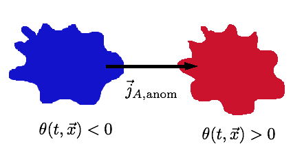
To decipher the nature of “ domain” through vector charge separation effects such as CME, it is essential to understand not only the distribution of those chiral charge imbalance, but their dynamical evolution as well. Previously, most studies were based on introducing chiral asymmetry by hand, after which the equilibrium response to a magnetic field (or vorticity) is investigated (see Ref. Fukushima et al. (2010) for the case in which the chirality is generated dynamically due to a particular color flux tube configuration). In reality, such as in heavy-ion collisions experiment, however, the chiral imbalance is dynamically generated through the presence of “ domain”. In this letter, we study the axial current induced by inhomogeneity of “ domain”, which can be conveniently described by introducing a space-time dependent angle (c.f. Refs. Kharzeev and Zhitnitsky (2007); Kharzeev et al. (2008)). One may interpret as an effective axion field creating a “ domain”. We show that the presence of will not only generate chiral charge imbalance, it will also lead to an axial current (c.f. Fig. 1):
| (3) |
Such an axial current, to best of knowledge, has not been considered in literature so far.
As it will be shown later, our results are valid as far as the variation of in space is on the scale larger than (or mean free path of the system) and the variation of in time is on the scale longer than the relaxation time of the system but shorter than the life time of “ domain”. It is therefore independent of the microscopic details of the system. While we are considering a system which is in the deconfined phase of QCD, the resulting current bears a close resemblance to that in the superfluid. One may interpret the gradient in Eq. (3) as the “velocity” of “ domain”, similar to the case of superfluid that the gradient of the phase of the condensate is related to the superfluid velocity. Moreover, we will show that the changing rate is related to the axial chemical potential appearing in the chiral magnetic current again similarly to the “Josephson-type equation” in superfluid. The relation between and is suggested in Ref. Fukushima et al. (2008). We will show how such a connection is realized in a non-trivial way.
The axial current in the presence of .—In this section, we will derive Eq. (3) and the constitute relation of in the presence of . The expectation value of induced by in Fourier space, is given by where is the retarded correlator of the density of topological charge density . For (or inverse of the mean free path), one may expand up to :
| (4) |
Here the first term is the topological susceptibility. It is highly suppressed in de-confined phase, as indicated by both lattice measurement and holographic calculation Bonati et al. (2014); Bergman and Lifschytz (2007). We will ignore from below. in the second term is the Chern-Simons diffusion rate and and are new transport coefficients. Combining Eq. (4) and the anomaly relation (2), we have in real space :
| (5) |
To proceed, we divide into two parts: . Here, we require to satisfy anomaly equation, i.e. , . Consequently, the remaining part is conserved: . In general, the above division is not unique. However, if we further require that to be local in , i.e. must be expressed in terms of and its gradients, can then be determined uniquely from Eq. (5) as follows. We start our analysis with . By taking the static limit of Eq. (5) and noting transforms as a vector under spatial rotation, one finds that have to be expressed in gradient of with the magnitude fixed by Eq. (5):
| (6) |
as was advertised earlier. Similarly, taking the homogeneous limit of Eq. (5) gives zeroth component of :
| (7) |
It is worth pointing out that appearing in Eq. (4) is accessible by the lattice. To see that, we note in the static limit
| (8) |
It is related to the Euclidean correlator by , which promises the possibility of measuring on the lattice through the following Kubo-formula:
| (9) |
At zero temperature, would coincide with the so-called “zero-momentum slope” of topological correlation function and is of phenomenological relevance in connection with the spin content of the proton (see Ref. Vicari and Panagopoulos (2009) and reference therein). However, the importance of in de-confined phase of QCD , to best of our knowledge, has not yet been appreciated. While is highly suppressed in de-confined phase, there is no reason for the suppression of . Eq. (6) gives an explicit example where is phenomenologically relevant.
Chiral charge imbalance, axial chemical potential and the real time dynamics of .—We are now ready to quantify the chiral charge imbalance due to the presence of . We concentrate on the first term on the R.H.S. of Eq. (7) and define axial density generated by as:
| (10) |
Eq. (10) implies that a local “ domain(bubble)” will induce a local axial charge density. Further insight can be obtained by looking at the axial chemical potential corresponding to in Eq. (10). Using the linearized equation of state where is the susceptibility, we have:
| (11) |
where we have introduced the sphaleron damping rate , which can be related to the Chern-Simon diffusion rate by the standard fluctuation-dissipation analysis Rubakov and Shaposhnikov (1996) (see also Iatrakis et al. (2015)): . Eq. (11) relating and is new in literature. It can be connected to the argument of Ref. Fukushima et al. (2008) in which is identified with . Eq. (11) implies that due to dynamical effects, one should replace in the identification with , the characteristic time scale of sphaleron damping. The above analysis suggests that while relation Eqs. (10),(11) have already captured the real time dynamics of the effective axion field , namely the sphaleron damping.
Finally, let us briefly comment on the conserved part of the axial current . Due to diffusion, we expect from Eq. (10) that:
| (12) |
The conservation of normal part determines the time component as . It depends on the history of normal part current, thus non-local in . It is also higher order compared to . For positive , axial current induced by “ domain” (3) is opposite to the diffusive current (12). We now argue that is always positive by noting that a non-zero will shift the action of the system by . Using the expression for in Eq. (8), one finds that in the static limit, . Therefore might be interpreted as coefficient of kinetic term of “axion field” and must be positive 111We stress that our field originates from topological fluctuation of gluons. It should not be confused with field from fermionic quasi-zero mode in Kalaydzhyan (2013).
The holographic model.—The discussion above does not rely on the microscopic details of the theory. We would like to confirm our findings in a top-down holographic model, namely, Sakai-Sugimoto model Sakai and Sugimoto (2005a, b), which at low enegy is dual to the four-dimensional Yang-Mills with massless quarks in large and strong coupling. The deconfined phase of the field theory is dual to the black-brane metric, which is a warped product of a black hole and , Witten (1998); Aharony et al. (2007). For the present work, we will consider field fluctuations with trivial dependence on , thus we only need the black hole part of the metric:
| (13) |
where and is the holographic coordinate with the boundary and the horizon. are related to the temperature of the system by . The flavor degrees of freedom are introduced by a pair of probe branes, separated along the direction, Sakai and Sugimoto (2005a). The probe branes do not back-react on the geometry.
We will compute axial density and axial current along one particular spatial direction, say “x” direction in the presence of a source, . To this end, we consider excitation of axial gauge field of the branes, with its field strength and Ramond-Ramond form. The index runs over and the rest of the components can be consistently set to zero. The source is related to , the component of along by , where is the radius of . Following the holographic correspondence, the axial current is dual to the axial gauge field, and the topological charge density is dual to . In the presence of , we consider instead components of Ramond-Ramond form(c.f. Ref. Sakai and Sugimoto (2005a)) . The field strength of , , is related to combination of by: 222The Levi-Civita symbol is fixed by . by Hodge duality between form and form. Here and with the ’t Hooft coupling.
After integrating over and noting fields depend only on , we obtain the effective action, which contains kinetic terms of and Wess-Zumino coupling between and Iatrakis et al. (2015):
| (14) |
In action (14), The indices in Eq. (14) are raised by 5d black hole part of the full metric. The equations of motion following from (14) are given by
| (15) |
According to holographic correspondence, the one point functions are given by the functional derivative of the gravity on-shell action with respect to the boundary values of . Using (Axial current generation by -odd domains in QCD matter), we can then express in terms of :
| (16) |
We now need to solve the bulk equation of motion for and (see Eq. (18) and Eq. (19) below) with appropriate boundary condition. We impose the infalling wave condition at the black hole horizon. On the boundary, has the following asymptotic expansion
| (17) |
The term is proportional to and the constant term gives . One could verify that (Axial current generation by -odd domains in QCD matter) and (17) indeed reproduce the anomaly equation: . We only keep the constant term in near boundary expansion of in the limit. The divergent terms should be removed by holographic renormalization procedure: e.g. the factor in the leading term, which is completely determined by the near boundary behavior of bulk equation of motion, indicates that it is a contact term that can be subtracted by a boundary counter term. In case of non-conformal backgrounds, as the Witten-Sakai-Sugimoto bulk space-time, the holographic renormalization procedure is carefully described in Kanitscheider et al. (2008). On the other hand, is not sourced on the boundary, thus we set . Note that , The back-reaction of to is suppressed. Keeping leading contribution in , we find the following equations of motion for and from action (14):
| (18) |
| (19) |
Results of holographic calculation.— We are interested in the solutions to Eq. (18) and Eq. (19) in hydrodynamic regime, i.e., . They can be found analytically, order by order in , following standard procedure in literature (c.f. Refs. Kovtun and Starinets (2005); Iqbal and Liu (2009)). The full expressions and details of the calculations are straightforward but lengthy and will be reported in a forthcoming paper Iatrakis et al. (2015). In order to compute , we only need their near-boundary expansions:
| (20) |
| (21) |
where . From Eq. (20), we immediately read by using Eq. (17). Further comparison with Eq. (5) gives in Sakai-Sugimoto model333 The value of CS diffusion rate has already been calculated in Ref. Craps et al. (2012). Our value is four times the value computed in Ref. Craps et al. (2012) due to a different normalization. :
| (22) |
where is the mas gap of the theory. Now plugging Eq. (20) and Eq. (21) into Eqs. (Axial current generation by -odd domains in QCD matter), we recover the time component of axial current in Eq. (10) and spatial component as a sum of Eq. (6) and (12):
| (23) |
where the diffusion constant in Sakai-Sugimoto model Yee (2009).
Phenomenological implication in heavy-ion collisions.— In this letter, we found a new mechanism for generating axial current (3) due to the inhomogeneity of effective “ domains”. We now estimate its magnitude in a hot QGP and examine its phenomenological importance in heavy-ion collisions. We start by relating to using Eq. (11). In terms of , the characteristic size of a “ domains”, Eq. (3) can be then estimated as:
| (24) |
where in the last step we have taken our holographic results (22) which implies as a crude estimate of in QCD plasma.
We now compare Eq. (24) to axial current from other sources. For QGP in the presence of magnetic field, axial current can be generated by chiral charge separation effects(CCSE) Son and Zhitnitsky (2004); *Metlitski:2005pr. Similar to CME, the CCSE current is given by . In heavy-ion collisions at top RHIC energy, at early stage is of a few and consequently is at most the same order as . Moreover, in those collisions, most of (or ) is generated from fluctuations and is expected to be the same order as . We therefore conclude that axial current is at least comparable to CCSE current if but could be larger if . A similar argument also applies to the comparison to chiral electric separation effect Huang and Liao (2013).
The axial current (3) studied in this work is induced by topological fluctuation. In plasma with chiral charge, axial charge can also be generated by thermal fluctuation, which is non-topological. Axial current can also exist as diffusion of such charge. Assuming the corresponding is the same order as the one from topological fluctuation, we can estimate the current as
| (25) |
where is mean free path of fermions and we have taken and . Comparing with Eq. (24), we conclude if the “ domain” parameter is larger than , the current (3) would dominate over axial current generated by thermal diffusion.
To sum up, if the condition is achieved heavy-ion collisions, the new current (3) proposed in this paper would become phenomenologically important.
Acknowledgments.— The authors would like to thank U. Gursoy, C. Hoyos, D. Kharzeev, E. Kiritsis, K. Landsteiner, L. McLerran, G. Moore, R. Pisarski, E. Shuryak, H-U. Yee and I. Zahed for useful discussions and the Simons Center for Geometry and Physics for hospitality where part of this work has been done. I.I. would also like to thank the Mainz Institute for theoretical Physics for the hospitality and partial support during the last stage of this work. This work is supported in part by the DOE grant No. DE-FG-88ER40388 (I.I.) and in part by DOE grant No. DE-SC0012704 (Y.Y.) . S.L. is supported by RIKEN Foreign Postdoctoral Researcher Program.
References
- Manton (1983) N. Manton, Phys.Rev. D28, 2019 (1983).
- Klinkhamer and Manton (1984) F. R. Klinkhamer and N. Manton, Phys.Rev. D30, 2212 (1984).
- Kuzmin et al. (1985) V. Kuzmin, V. Rubakov, and M. Shaposhnikov, Phys.Lett. B155, 36 (1985).
- Shaposhnikov (1987) M. Shaposhnikov, Nucl.Phys. B287, 757 (1987).
- Arnold and McLerran (1987) P. B. Arnold and L. D. McLerran, Phys.Rev. D36, 581 (1987).
- Arnold and McLerran (1988) P. B. Arnold and L. D. McLerran, Phys.Rev. D37, 1020 (1988).
- Zhitnitsky (2012a) A. R. Zhitnitsky, Phys.Rev. D86, 045026 (2012a), arXiv:1112.3365 [hep-ph] .
- Zhitnitsky (2012b) A. R. Zhitnitsky, Nucl.Phys. A886, 17 (2012b), arXiv:1201.2665 [hep-ph] .
- Zhitnitsky (2013) A. R. Zhitnitsky, Annals Phys. 336, 462 (2013), arXiv:1301.7072 [hep-ph] .
- Kharzeev and Zhitnitsky (2007) D. Kharzeev and A. Zhitnitsky, Nucl.Phys. A797, 67 (2007), arXiv:0706.1026 [hep-ph] .
- Liao (2014) J. Liao, (2014), arXiv:1401.2500 [hep-ph] .
- Chao et al. (2013) J. Chao, P. Chu, and M. Huang, Phys.Rev. D88, 054009 (2013), arXiv:1305.1100 [hep-ph] .
- Yu et al. (2014) L. Yu, H. Liu, and M. Huang, Phys.Rev. D90, 074009 (2014), arXiv:1404.6969 [hep-ph] .
- Fukushima et al. (2008) K. Fukushima, D. E. Kharzeev, and H. J. Warringa, Phys. Rev. D 78, 074033 (2008), arXiv:0808.3382 [hep-ph] .
- Kharzeev (2014) D. E. Kharzeev, Prog.Part.Nucl.Phys. 75, 133 (2014), arXiv:1312.3348 [hep-ph] .
- Fukushima et al. (2010) K. Fukushima, D. E. Kharzeev, and H. J. Warringa, Phys.Rev.Lett. 104, 212001 (2010), arXiv:1002.2495 [hep-ph] .
- Kharzeev et al. (2008) D. E. Kharzeev, L. D. McLerran, and H. J. Warringa, Nucl.Phys. A803, 227 (2008), arXiv:0711.0950 [hep-ph] .
- Bonati et al. (2014) C. Bonati, M. D’Elia, H. Panagopoulos, and E. Vicari, PoS LATTICE2013, 136 (2014), arXiv:1309.6059 [hep-lat] .
- Bergman and Lifschytz (2007) O. Bergman and G. Lifschytz, JHEP 0704, 043 (2007), arXiv:hep-th/0612289 [hep-th] .
- Vicari and Panagopoulos (2009) E. Vicari and H. Panagopoulos, Phys.Rept. 470, 93 (2009), arXiv:0803.1593 [hep-th] .
- Rubakov and Shaposhnikov (1996) V. Rubakov and M. Shaposhnikov, Usp.Fiz.Nauk 166, 493 (1996), arXiv:hep-ph/9603208 [hep-ph] .
- Iatrakis et al. (2015) I. Iatrakis, S. Lin, and Y. Yin, (2015), arXiv:1506.01384 [hep-th] .
- Note (1) We stress that our field originates from topological fluctuation of gluons. It should not be confused with field from fermionic quasi-zero mode in Kalaydzhyan (2013).
- Sakai and Sugimoto (2005a) T. Sakai and S. Sugimoto, Prog.Theor.Phys. 113, 843 (2005a), arXiv:hep-th/0412141 [hep-th] .
- Sakai and Sugimoto (2005b) T. Sakai and S. Sugimoto, Prog.Theor.Phys. 114, 1083 (2005b), arXiv:hep-th/0507073 [hep-th] .
- Witten (1998) E. Witten, Adv.Theor.Math.Phys. 2, 505 (1998), arXiv:hep-th/9803131 [hep-th] .
- Aharony et al. (2007) O. Aharony, J. Sonnenschein, and S. Yankielowicz, Annals Phys. 322, 1420 (2007), arXiv:hep-th/0604161 [hep-th] .
- Note (2) The Levi-Civita symbol is fixed by .
- Kanitscheider et al. (2008) I. Kanitscheider, K. Skenderis, and M. Taylor, JHEP 0809, 094 (2008), arXiv:0807.3324 [hep-th] .
- Kovtun and Starinets (2005) P. K. Kovtun and A. O. Starinets, Phys.Rev. D72, 086009 (2005), arXiv:hep-th/0506184 [hep-th] .
- Iqbal and Liu (2009) N. Iqbal and H. Liu, Phys.Rev. D79, 025023 (2009), arXiv:0809.3808 [hep-th] .
- Note (3) The value of CS diffusion rate has already been calculated in Ref. Craps et al. (2012). Our value is four times the value computed in Ref. Craps et al. (2012) due to a different normalization.
- Yee (2009) H.-U. Yee, JHEP 0911, 085 (2009), arXiv:0908.4189 [hep-th] .
- Son and Zhitnitsky (2004) D. Son and A. R. Zhitnitsky, Phys.Rev. D70, 074018 (2004), arXiv:hep-ph/0405216 [hep-ph] .
- Metlitski and Zhitnitsky (2005) M. A. Metlitski and A. R. Zhitnitsky, Phys.Rev. D72, 045011 (2005), arXiv:hep-ph/0505072 [hep-ph] .
- Huang and Liao (2013) X.-G. Huang and J. Liao, Phys.Rev.Lett. 110, 232302 (2013), arXiv:1303.7192 [nucl-th] .
- Kalaydzhyan (2013) T. Kalaydzhyan, Nucl.Phys. A913, 243 (2013), arXiv:1208.0012 [hep-ph] .
- Craps et al. (2012) B. Craps, C. Hoyos, P. Surowka, and P. Taels, JHEP 1211, 109 (2012), arXiv:1209.2532 [hep-th] .