Precision–Energy–Throughput Scaling Of Generic Matrix Multiplication and Convolution Kernels Via Linear Projections

Abstract

Generic matrix multiplication (GEMM) and one-dimensional convolution/cross-correlation (CONV) kernels often constitute the bulk of the compute- and memory-intensive processing within image/audio recognition and matching systems. We propose a novel method to scale the energy and processing throughput of GEMM and CONV kernels for such error-tolerant multimedia applications by adjusting the precision of computation. Our technique employs linear projections to the input matrix or signal data during the top-level GEMM and CONV blocking and reordering. The GEMM and CONV kernel processing then uses the projected inputs and the results are accumulated to form the final outputs. Throughput and energy scaling takes place by changing the number of projections computed by each kernel, which in turn produces approximate results, i.e. changes the precision of the performed computation. Results derived from a voltage- and frequency-scaled ARM Cortex A15 processor running face recognition and music matching algorithms demonstrate that the proposed approach allows for $280\%\sim 440\%$ increase of processing throughput and $75\%\sim 80\%$ decrease of energy consumption against optimized GEMM and CONV kernels without any impact in the obtained recognition or matching accuracy. Even higher gains can be obtained if one is willing to tolerate some reduction in the accuracy of the recognition and matching applications.

I Introduction

Error-tolerant multimedia processing [1] comprises any system that: (i) processes large volumes of input data (image pixels, sensor measurements, database entries, etc.) with performance-critical digital signal processing (DSP) or linear algebra kernels (filtering, decomposition, factorization, feature extraction, principal components, probability mixtures, Monte-Carlo methods, etc.) and (ii) the quality of its results is evaluated in terms of minimum mean-squared error (MSE) or maximum learning, recognition or matching rate against ground-truth or training data, rather than performance bounds for individual inputs. Examples of such error-tolerant (ET) systems include: lossy image/video/audio compression [2, 3], computer graphics [4, 5], webpage indexing and retrieval [6], object and face recognition in video [7, 8], image/video/music matching [9, 10, 11, 12], etc. For instance, all face recognition and webpage ranking algorithms optimize for the expected recall percentage against ground-truth results and not for the worst-case. This is also because typical input data streams comprise noisy entries originating from audio/visual sensors, web-crawlers, field-measurement microsensors, etc. Therefore, ET applications have to tolerate approximations in their results, and can use this fact to reduce computation time or energy consumption [1].

Two of the most critical linear algebra and DSP kernels used in ET applications are the generic matrix multiplication (GEMM) and one-dimensional convolution/cross-correlation (CONV) kernels. This paper proposes a new approach to systematically scale the computation time and energy consumption of optimized GEMM and CONV kernels within ET applications with minimal or no effect in their results.

I-A Previous Work

Several papers have studied techniques to trade-off approximation versus implementation complexity in GEMM and CONV computations within special-purpose systems. Starting with theory-inspired approaches for approximate GEMM and CONV kernel realization, Monte-Carlo algorithms have been proposed for fast approximate matrix multiplication suitable for massive dataset processing on networked computing systems (aka “Big Data” systems) [13], such as Google MapReduce and Microsoft Dryad. The concepts of approximate and stochastic computation in custom hardware were proposed as a means to achieve complexity-distortion scaling in sum-of-products computations [14]. Approximate convolution operations in conjunction with voltage overscaling in custom hardware was proposed recently within the framework of stochastic computation [15].

Other works focus on performance vs. precision tradeoffs of GEMM and CONV kernels within specific algorithms. For example, Merhav and Kresch [16] presented a novel method of approximate convolution using discrete cosine transform (DCT) coefficients, which is appropriate only for DCT-domain processing. Chen and Sundaram [17] proposed a polynomial approximation of the input signal for accelerated approximate Fast Fourier Transform (FFT) computations. Di Stefano and Mattoccia [18] presented an accelerated normalized spatial-domain cross-correlation mechanism, with partial check according to an upper bound. Finally, Kadyrov and Petrou [19] and Anastasia and Andreopoulos [20] showed that it is possible to perform accelerated 2D convolution/cross-correlation by piecewise packing of the input image data into a compact representation when the algorithm utilizes integer inputs.

A third category of research advances on GEMM and CONV energy and processing throughput adaptation is focusing on specific error-tolerant applications, such as video codecs, image processing and signal processing operations in custom hardware designs [21, 22, 23, 24, 25, 26, 27, 28, 29, 30]. Beyond their reliance to specialized hardware or circuit design for complexity–precision scalability of GEMM and CONV kernels, many such approaches also tend to be algorithm-specific. That is, they use predetermined “quality levels” or “profiles” of algorithmic or system adjustment, e.g.: switching to simpler transforms or simplifying algebraic operations [4][31][32], limiting the operating precision of the algorithm implementation in a static manner in order to satisfy hardware or processing constraints [33], or exploiting the structure of matrices in sparse matrix problems [34]. Previous research efforts by our group in image processing systems [35, 20] were also algorithm-specific and, importantly, no precision-controlled acceleration of linear operations was proposed. For these reasons, many existing proposals of this category [13, 36, 15, 37, 38, 17] are either based on complexity models or custom VLSI designs and cannot be easily generalized to mainstream digital signal processors or high-performance computing clusters.

Overall, all current approaches for precision–energy–throughput scaling of GEMM and CONV kernels appear to be limited by one or more of the following: (i) adaptation is only done at the process level (e.g. results of entire tasks are dropped); (ii) the proposed methods are tailored to specific algorithms (e.g. image filtering or specific signal transforms); (iii) special-purpose hardware is required and optimized deployment via mainstream processors with streaming single-instruction multiple-data (SIMD) extensions is not possible.

I-B Contribution

This paper proposes an approach to scale precision, energy and throughput (PET) scaling in GEMM and CONV kernels that form the dominant compute and memory-intensive processing within broad classes of image/audio recognition or matching systems. Our proposal is applicable to GEMM and CONV kernels running on commercial off-the-shelf processors and, via PET scaling, it is shown to significantly outperform state-of-the-art deployments on such processors. Importantly, PET scaling in our approach is done with straightforward selection of a few parameters that are software-adjustable. Finally, our approach is not limited to a specific algorithm or application; rather it is applicable to a large range of ET applications based on GEMM and CONV kernels.

To illustrate how these important advantages are achieved by our proposal, Figure 1 presents a schematic layering of the execution of typical compute and memory-intensive ET multimedia applications on high-performance and embedded systems. As shown in the figure, between L2 and L3, a partitioning [39] (or reordering [40, 41]) of the input data takes place and each data block is assigned to a kernel-processing core (or thread) for memory-efficient (and, possibly, concurrent) realization of subsets of GEMM and CONV computations. Each core returns its output block of results to the top-level processing of L2 and all blocks are assembled together to be returned to the high-level algorithm. Parallelism and data movement to and from cores tend to increase drastically between L2 and L3.

When aiming for high-throughput/low-energy performance, the critical issues of the execution environment of Figure 1 are [1, 40, 41]: (i) the data movement to/from cores; (ii) the processing time and energy consumption per core; (iii) the limited concurrency when the top-level processing allows for only a few blocks. These issues are addressed in our proposal by viewing the process between L2 and L3 as a computation channel [39] that returns approximate results. All current approaches correspond to the least-efficient, “lossless”, mode (i.e. typically 32-bit floating-point accuracy), which will typically be unable to accommodate timing and/or energy constraints imposed by the application. It is proposed to create highly-efficient, “lossy”, modes for pre- and post-processing of streams via projection techniques (L2.5 of Figure 1). This is achieved by: (i) partitioning and reordering inputs in L2 to move them to each core for kernel processing; (ii) converting them into multiple, compact, representations allowing for reduced data movement, increased concurrency and fast recovery of approximate results from only a few cores.

I-C Paper Organization

In Section II, we review the top-level processing of GEMM and CONV kernels considered in this paper. Section III presents the proposed projections-based data compaction method within GEMM and CONV kernels. Section IV presents performance benchmarks for the proposed method in terms of precision, energy consumption and processing throughput attained on the recently-introduced ARM Cortex A15 processor. In addition, comparisons against both the original (i.e. non projections-based) kernels, as well as state-of-the-art GEMM and CONV kernels from third parties, are carried out. Section V demonstrates the ability of the proposed approach to achieve substantial resource–precision adaptation within two error-tolerant multimedia recognition and matching applications. Finally, Section VI concludes the paper.

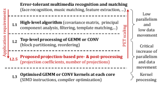
Figure 1: Proposed work positioned within the execution environment of ET multimedia applications.

II Overview of Top-level Processing of GEMM and CONV Kernels

This section outlines the key aspects of data partitioning and reordering within the GEMM and CONV kernels under consideration. Specifically, the accessing and partitioning order of the input data streams is shown, in order to provide the context under which the proposed projections-based mechanisms are deployed. The nomenclature summary of this paper is given in Table I.

Table I: Nomenclature table.

Symbol	Definition
$M$, $K$, $W$	Input matrix or signal size parameters
$N$	Kernel size (e.g. $N\times N$ subblock in GEMM or $N$-sample convolution kernel)
$L$	Total number of projections used
$\mathbf{A}_{i}$, $\mathbf{a}$, $\mathbf{A^{\mathbf{T}}}$	Boldface uppercase and lowercase letters indicate matrices and vectors, respectively; superscript T denotes transposition
$\widehat{r}_{\text{sub}}$	Reconstruction of result $r$ using subset “sub” of projections
$a\left[0,0\right]$	Italicized lowercase letters indicate elements of corresponding matrices or vectors (with the enumeration starting from zero)
$\left\|\mathbf{A}\right\|_{F}$	Frobenius norm
a$\leftarrow$instr(b,c)	Indicates assignment of result to variable a after performing instruction instr using b and c (the meaning of the instruction is identifiable from the context) in pseudocode listings

II-A Brief Review of Block Processing within GEMM

Consider the standard GEMM design depicted in Figure 2, following the general flow found in optimized MKL designs [40, 41]. The application invokes GEMM for an $M\times K$ by $K\times W$ matrix multiplication that is further subdivided into $N\times N$ “inner-kernel” matrix products. For our approach, $N$ is specified by ($k\in\mathbb{N}^{\star}$):

$$N=2k\times\frac{\text{SIMD}_{\text{bits}}}{b_{\text{repr}}}$$ (1)

with: $\text{SIMD}_{\text{bits}}$ the number of bits of each SIMD register ($\text{SIMD}_{\text{bits}}=128$ in this work); $b_{\text{repr}}=32$ the number of bits for floating-point or integer (fixed-point) representations. The inner-kernel result, $\mathbf{R}_{2,1}$, of the example shown in Figure 2 comprises the sum of multiple subblock multiplications $\mathbf{A}_{2,n}\mathbf{B}_{n,1}$, and is given by:

$$\mathbf{R}_{2,1}=\sum_{n=0}^{\frac{K}{N}-1}\mathbf{A}_{2,n}\mathbf{B}_{n,1}.$$ (2)

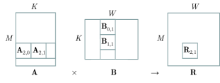
Figure 2: Top-level processing of GEMM highlighting the input subblocks involved in the example subblock result $\mathbf{R}_{2,1}$.

If the matrices’ dimensions are not multiples of $N$, some “cleanup” code [40, 41] is applied at the borders to complete the inner-kernel results of the overall matrix multiplication. This separation into top-level processing and subblock-level processing is done for efficient cache utilization [41, 42]. Specifically, during the initial data access of GEMM for top-level processing, data in matrix $\mathbf{A}$ and $\mathbf{B}$ is reordered into block major format: for each $N\times N$ pair of subblocks $\mathbf{A}_{i,n}$ and $\mathbf{B}_{n,j}$ multiplied to produce inner-kernel result $\mathbf{R}_{i,j}$, $0\leq n<\frac{K}{N}$, $0\leq i<\frac{M}{N}$, $0\leq j<\frac{W}{N}$, the input data within $\mathbf{A}_{i,n}$ and $\mathbf{B}_{n,j}$ is reordered in rowwise and columnwise raster manner, respectively. Thus, sequential data accesses are performed during each subblock matrix multiplication and this enables the use of SIMD instructions, thereby leading to significant acceleration. The appropriate value for the subblock dimension, $N$, can be established for each architecture following an automated process at compile time (e.g. via test runs [69]).

Our approach intercepts the subblock-based rowwise and columnwise raster ordering (exploiting the fact that the input data subblock is accessed anyway) in order to perform low-complexity linear projections to the input rows and columns prior to the performance of individual GEMMs within the projected data. In conjunction with the fact that the proposed approach does not alter the top-level processing of the standard GEMM, in the remainder of the paper we only refer to a single subblock product. For notational simplicity, we remove the indices from subblock product $\mathbf{A}_{i,n}\mathbf{B}_{n,j}$.

II-B Brief Review of Overlap-save Processing within CONV

Consider the discrete convolution of two 1D signals, $\mathbf{s}_{\text{in}}$ and $\mathbf{k}$, producing the output signal, $\mathbf{r}_{\text{out}}$:

$$\mathbf{r}_{\text{out}}=\mathbf{s}_{\text{in}}\star\mathbf{k}\Longleftrightarrow\forall m:\;r_{\text{out}}\left[m\right]=\sum_{n=0}^{N-1}s_{\text{in}}\left[n\right]k\left[m-n\right].$$ (3)

The signal with the smallest time-domain support is considered to be the kernel, $\mathbf{k}$, and the other signal, $\mathbf{s}_{\text{in}}$, is the input. Assuming $\mathbf{s}_{\text{in}}$ is periodic with period $N$, circular convolution of period $N$ can be expressed by:

$$\mathbf{r}_{\text{out}} = \left(\mathbf{s}_{\text{in}}\circledast\mathbf{k}\right)_{N}\Longleftrightarrow$$

$$\forall m:\;r_{\text{out}}\left[m\right] = \sum_{n=0}^{N-1}\left(\sum_{p=-\infty}^{\infty}s_{\text{in}}\left[n+pN\right]\right)k\left[m-n\right]$$ (4)

Finally, discrete cross-correlation and circular cross-correlation can be obtained by replacing $k\left[m-n\right]$ with $k\left[m+n\right]$ in (3) and (4).

As shown in Figure 3, practical implementations of convolution of a long input signal with an $N$-sample kernel $\mathbf{k}$ will subdivide the input into several partially-overlapping blocks—of $W$ samples each (vector $\mathbf{s}$)—prior to the actual convolution. Each individual signal block $\mathbf{s}$ is independently convolved with the kernel and the resulting blocks ($\mathbf{r}$) are assembled together to give the result of the convolution. This is the well-known overlap-save method [43], performed for efficient cache utilization and increased concurrency, with the degree of concurrency and the processing delay depending on $W$. The optimal value of $W$ for the utilized architecture can be derived based on offline experimentation, e.g., during the routine compilation or via offline experiments with the target processor [44].

Our approach exploits the fact that overlap-save CONV accesses blocks of data (in order to subdivide the input) and applies low-complexity projection operations during this process. Similarly, as for the case of GEMM, in the next section we shall only be presenting the proposed method for one block of $W$ samples and, for notational simplicity, we shall not retain the block index but rather consider it to be the entire input signal $\mathbf{s}_{\text{in}}$.

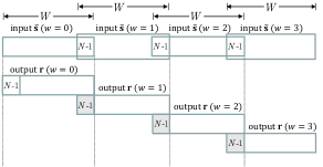
Figure 3: Top-level processing of CONV highlighting the overlap-save method.

III PET Scaling of Numerical Kernels via Linear Projections

We first present an example of how projections in numerical kernels produce a hierarchical representation of inner-product computations, which comprise the core operation within both kernels. In Subsection III-B we elaborate on the deployment of the proposed projections-based resource–precision scaling within high-performance GEMM and CONV kernels. Finally, in Subsection III-C we quantify its multiply–accumulate (MAC) operations and required data transfers between top-level and kernel processing against the standard kernel realization that does not use projections.

III-A Illustration of the Basic Concept

Consider the calculation of an inner product $r=\mathbf{a}\mathbf{b}$, such as the one illustrated in the example of the top half of Figure 4. We can apply projection matrices $\mathbf{C}$ and $\mathbf{D}$ to the inputs by:

$$\mathbf{a}_{c}=\mathbf{a}\mathbf{C},\;\;\mathbf{b}_{d}=\mathbf{D}\mathbf{b}$$ (5)

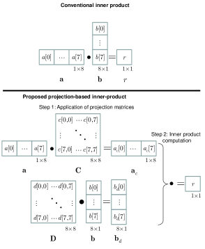
Figure 4: Eight-sample inner product computation using $8\times 8$ projection matrices $\mathbf{C}$ and $\mathbf{D}$. Top half: inner product computation. Bottom half: projections-based inner product.

If $\mathbf{C}$ is an invertible square matrix and we set $\mathbf{D}=\mathbf{C}^{-1}$, the inner product can take place using the projected vectors, since:

$$\mathbf{a}_{c}\mathbf{b}_{d}=\left(\mathbf{a}\mathbf{C}\right)\left(\mathbf{D}\mathbf{b}\right)=\mathbf{a}\mathbf{\left(CD\right)}\mathbf{b}=\mathbf{ab}=r$$ (6)

which is illustrated in the bottom half of Figure 4. If one ignores the cost of performing the projections of (5), the inner product of (6) incurs the same computational effort as the original inner product. Importantly, the projection matrices can prioritize the computation of the result since, if appropriately selected, they can concentrate the energy of the inputs in the first few elements. For example, considering that the input vectors $\mathbf{a}$ and $\mathbf{b}$ comprise image or signal data with energy concentrated in low frequencies and $\mathbf{C}$ is chosen as the $L$-point discrete cosine transform (DCT) transform ($L=8$, $\forall i,j:\>0\leq i,j<8$):

$$c\left[i,j\right]=\cos\left[\frac{\pi}{L}\left(i+\frac{1}{2}\right)j\right],$$ (7)

if we only perform $\widehat{r}_{\text{DC}}=a_{c}\left[0\right]b_{d}\left[0\right]$, this corresponds to reconstructing the “DC component” of the entire inner product of (6). In addition, this can optionally be incremented up to the eighth harmonic (i.e., reconstructing $r$ up to—and including—the eighth harmonic) by:

$$\widehat{r}_{\text{full}}=\sum_{l=0}^{7}a_{c}\left[l\right]b_{d}\left[l\right].$$ (8)

with $\widehat{r}_{\text{full}}=r$ barring numerical approximation error. The computation of each harmonic $a_{c}\left[l\right]b_{d}\left[l\right]$ can be assigned to a different processor and the accumulation of (8) is optional: if less than all eight harmonics are accumulated, the precision of the result is expected to degrade gracefully. This reduces the energy consumption and data transfers to and from processors, or increases processing throughput if a single processor is used.

For a population of $N$ results ($0\leq n<N$), e.g., $r\left[n\right]=\mathbf{a}\mathbf{b}\left[n\right]$, the signal-to-noise ratio (SNR) between $r\left[0\right],\,\ldots,\,r\left[N-1\right]$ and $\widehat{r}_{\textrm{sub}}\left[0\right],\,\ldots,\,\widehat{r}_{\textrm{sub}}\left[N-1\right]$ (results computed in single-precision floating point vs. results reconstructed from subset “sub” of projections), is given by:

$$\text{SNR}=10\log_{10}\left(\frac{\sum_{n=0}^{N-1}r^{2}\left[n\right]}{\sum_{n=0}^{N-1}\left(r\left[n\right]-\widehat{r}_{\textrm{sub}}\left[n\right]\right)^{2}}\right).$$ (9)

If the projection matrices concentrate the energy of the input data in these projections, then the SNR of (9) can be adequately high for an error-tolerant multimedia application.

The extension of this simple example to inner products performed within matrix product computations is relatively straightforward to envisage. However, in the case of convolution/cross-correlation, due to the translations performed during the calculation of the results, we first need to define the cyclic permutation matrix comprising $N\times N$ elements [43]:

$$\mathbf{P}_{n}=\begin{bmatrix}\mathbf{0}&\mathbf{I}_{n}\\ \mathbf{I}_{N-n}&\mathbf{0}\end{bmatrix}$$ (10)

with: $0\leq n<N$, $\mathbf{I}_{k}$ the $k\times k$ identity matrix and $\mathbf{0}$ the zero matrix whose dimensions are identifiable from the context.

We can then define the projections-based circular cross-correlation operation for the example of Figure 4 based on the following steps:

1. For all translations $n$, $0\leq n<8$, derive the translated-and-projected inputs:
   

   $$\mathbf{a}_{c}\left[n\right]=\mathbf{a}\mathbf{P}_{n}\mathbf{C},$$ (11)

   with $\mathbf{a}_{c}\left[n\right]$ the $1\times 8$ vector corresponding to the projection of the $n$th cyclic translation (permutation) of $\mathbf{a}$.

2. Derive the projected input $\mathbf{b}_{d}$ by:
   

   $$\mathbf{b}_{d}=\mathbf{Db}.$$ (12)

3. Reconstruct the $\left(7-n\right)$th sample of the output by ($0\leq n<8$):
   

   $$\widehat{r}_{\text{full}}\left[7-n\right]=\mathbf{a}_{c}\left[n\right]\mathbf{b}_{d}=\sum_{l=0}^{7}a_{c}\left[n,l\right]b_{d}\left[l\right].$$ (13)

Circular convolution can be defined following the same steps if we reverse the order of either $\mathbf{a}$ or $\mathbf{b}$. Moreover, discrete convolution and cross-correlation are defined by these steps if extension with zeros is performed in (11) instead of cyclic permutations. Notice that well-known acceleration techniques like the FFT can be applied in (13) since, when considering all translations $n$, (13) comprises a variant of cross-correlation.

In the case of convolution, we have two options to scale performance. Firstly, we can opt to omit the calculation of some of the results of (13) and instead interpolate them from neighboring results, e.g. compute every other result and replace the missing ones by averaging the neighboring results. Secondly, we can opt to omit the calculation of some of the higher-numbered products within the summation of (13), which correspond to the higher harmonics of the translated-and-projected inputs. Both options will lead to approximate results, with the resulting error being quantified by the SNR calculation of (9). For instance, for the case of $\mathbf{C}$ being the $8\times 8$ DCT transform, we can reconstruct the DC component of the $\left(7-n\right)$th sample of the output by ($0\leq n<8$):

$$\widehat{r}_{\text{DC}}\left[7-n\right]=a_{c}\left[n,0\right]b_{d}\left[0\right].$$ (14)

III-B Application of the Concept within the Top-level Data Partitioning and Reordering of GEMM and CONV

For efficient deployment of projections-based processing within the blocked GEMM or CONV kernels, we must: (i) align the projection matrix size to the block size of each kernel and (ii) ensure the entire process is performed without breaking the access pattern of the data blocking (and possibly reordering) of the top-level processing of each kernel. The latter is important because this means the entire reordering and projections approach can be performed in a streaming manner, i.e. with high-performance SIMD instructions.

Assuming that the inner-kernel size comprises $N$ samples and the projection matrix comprises $L\times L$ coefficients, the first condition is satisfied if $N$ is divisable by $L$. For example, the values used in our experiments are: $N\in\left\{144,600,1200\right\}$ and $L\in\left\{2,8\right\}$.

Concerning the second condition, we first define the mathematical process of consecutive application of the projection kernels within each $N\times N$ GEMM subblock or each $N$-sample convolution kernel. This is achieved by defining the $N\times N$ block-diagonal matrices:

$$\mathbf{C}_{N}=\begin{bmatrix}\mathbf{C}&\mathbf{0}&\cdots&\mathbf{0}\\ \mathbf{0}&\mathbf{C}&&\mathbf{0}\\ \vdots&&\ddots&\vdots\\ \mathbf{0}&\mathbf{0}&\cdots&\mathbf{C}\end{bmatrix},\;\mathbf{D}_{N}=\begin{bmatrix}\mathbf{D}&\mathbf{0}&\cdots&\mathbf{0}\\ \mathbf{0}&\mathbf{D}&&\mathbf{0}\\ \vdots&&\ddots&\vdots\\ \mathbf{0}&\mathbf{0}&\cdots&\mathbf{D}\end{bmatrix},$$ (15)

with: $\mathbf{C}$ and $\mathbf{D}$ the $L\times L$ projection matrices, $\mathbf{C}$ comprising any invertible matrix and $\mathbf{D}=\mathbf{C}^{-1}$. The mathematical application of the projection process then follows the exposition of the previous subsection, albeit ignoring all elements of the projection operations that contain zero coefficients.

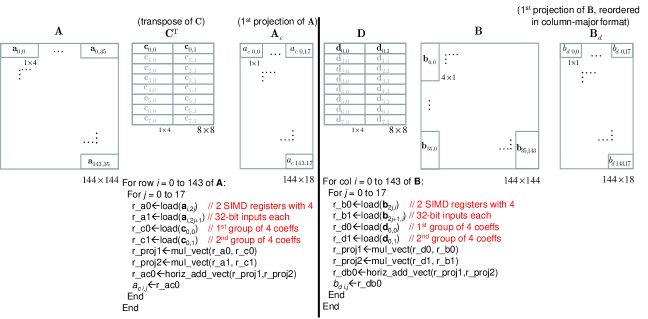
Figure 5: Application of first projection of $8\times 8$ projection matrices $\mathbf{C}$ and $\mathbf{D}$ during block-major reordering in GEMM under SIMD registers storing four 32-bit elements. Left half: right multiplication of blocks within the rows of $\mathbf{A}$ by all elements of the first row of $\mathbf{C}^{\text{T}}$ (which is equivalent to left-multiplying with the first column of $\mathbf{C}$). Right half: left multiplication of blocks within the columns of $\mathbf{B}$ by the first row of $\mathbf{D}$. The grayed-out rows of $\mathbf{C}^{\text{T}}$ and $\mathbf{D}$ correspond to the subsequent projections.

In order to illustrate how this can be done following the access pattern of the input data partitioning and reordering (and, more specifically, using with SIMD instructions), Figure 5 demonstrates one projection operation during the block-major reordering performed in GEMM. The figure illustrates the application of the first projection vector (first row of $\mathbf{C}^{\text{T}}$ and first row of $\mathbf{D}$) within a pair of subblocks of size $N\times N$. In this example, we selected $N=144$ and $L=8$ (i.e. eight projections, comprising eight coefficients each), which are the values used in our experiments. In addition, we left-multiply each row of $\mathbf{A}$ with each row of $\mathbf{C}^{\text{T}}$, which is equivalent to right-multiplying the rows of $\mathbf{A}$ with the columns of $\mathbf{C}$ but it is more efficient as all input elements are contiguous in memory (thereby allowing for the use of SIMD instructions). This is illustrated in the pseudocode of Figure 5, where we present simplified SIMD instructions used in the inner loop of the projection operation performed: mult_vect(r1,r2) multiplies two SIMD registers r1 and r2 and horiz_add_vect(r1,r2) adds all eight elements within r1 and r2 (each SIMD register has four 32-bit elements). Specifically, the realization of the first projection of the $j$th group of eight values in the $i$th row of $\mathbf{A}$ is performed via the following (pseudocode of the left part of Figure 5):

• the first two load instructions of the inner For loop load two pairs of four consecutive values of $\mathbf{A}$ into registers r_a0 and r_a1;

• the next two instructions load the two pairs of four consecutive projection coefficients of the first row of $\mathbf{C}^{\text{T}}$ into registers r_c0 and r_c1;

• two vector multiplications are then carried out (r_a0 $\times$ r_c0 and r_a1 $\times$ r_c1) and the results are stored in registers r_proj1 and r_proj2;

• the contents of these two registers are all added together to create the $\left(i,j\right)$th element of $\mathbf{A}_{c}$.

The equivalent process is carried out for the realization of the first projection of the $j$th group of eight values in the $i$th column of $\mathbf{B}$ (shown in the pseudocode of the right part of Figure 5).

As shown in Figure 5, this process results in a smaller GEMM product of dimensions $144\times 18$ by $18\times 144$. All eight projections can be derived by using the subsequent (grayed-out) rows of $\mathbf{C}^{\text{T}}$ and $\mathbf{D}$ and they can be performed independently in eight different processing cores. This results in: (i) eight-fold increase of concurrency/data-level parallelism within each subblock product, (ii) reduced data transfers to each core. Moreover, by computing only a small number of projections, e.g. just one to three, this approach allows for graceful degradation of the SNR of (9) under energy and throughput scaling.

Concerning the signal block partitioning during the top-level processing of CONV, in Figure 6 we demonstrate a single projection operation applied to the input signal $\mathbf{s}$ and kernel $\mathbf{k}$. Here, we utilize the following sizes for the signal, kernel and projections: $W=20000$, $N=600$ and $L=2$, which correspond to the values used in our experiments. In the pseudocode of Figure 6, load_dup($\mathbf{c}_{0}$) loads the two elements of $\mathbf{c}_{0}$ and duplicates them within one SIMD register and horiz_pairadd_vect(r) performs two pairwise additions within the four elements of r. Specifically, the realization of the projection of the $i$th group of four values in $\mathbf{s}$ is performed via the following:

• the first load instruction of the For loop loads four consecutive values of $\mathbf{s}$ into register r_s;

• the second load instruction loads and duplicates the two values of the first row of $\mathbf{C}$ into register r_c0;

• a vector multiplication is then carried out (r_s $\times$ r_c0) and the results are stored in register r_proj;

• the contents of this register are all added together to create the $i$th element of $\mathbf{s}_{c}$.

The equivalent process is carried out for the realization of the first projection of the $i$th group of four values in kernel $\mathbf{k}$.

Figure 5 shows that the projection leads to a convolution operation with half the number of samples in both the input signal and the kernel ($\mathbf{s}_{c}$ and $\mathbf{k}_{d}$, respectively), thereby asymptotically decreasing the arithmetic complexity by a factor of four. This can be extended to higher gains if higher values of $L$ are used.

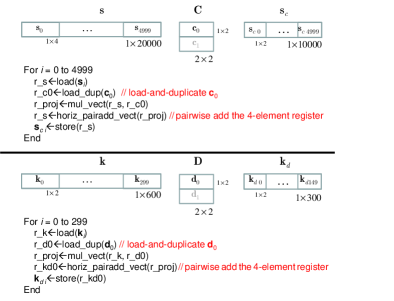
Figure 6: Application of projection operations during blocking of CONV. Top half: projection of input signal $\mathbf{s}$. Bottom half: projection of kernel $\mathbf{k}$.

III-C Computational and Memory Aspects of Projections-based GEMM and CONV

The conventional (or “plain”) GEMM kernel (i.e., without projections) requires

$$\text{C}_{\text{GEMM,plain}}\left(N\right)=N^{3}$$ (16)

MAC operations for each pair of $N\times N$ subblocks $\mathbf{A}$ and $\mathbf{B}$. On the other hand, for deriving $\left(l+1\right)$ projections out of the $L$ possible ones ($0\leq l<L$), $2\left(l+1\right)N^{2}$ MAC operations are performed in the input subblocks, followed by $\frac{l+1}{L}N^{3}$ MAC operations for the $\left(l+1\right)$ smaller matrix products, $\mathbf{A}_{c}\mathbf{B}_{d}$ (shown in Figure 5 for the first projection), and $lN^{2}$ accumulation operations to produce the final results. Thus, in total,

$$\text{C}_{\text{GEMM,proj}}\left(N,l,L\right)=N^{2}\left[\frac{l+1}{L}N+3l+2\right]$$ (17)

MAC operations are required for the proposed approach when performing $\left(l+1\right)$ projections of $L$ coefficients each. In terms of data transfer and storage requirements, the conventional GEMM requires $\text{M}_{\text{GEMM,plain}}=2N^{2}b_{\text{repr}}$ bits to be transferred to each GEMM subblock kernel [with $b_{\text{repr}}$ the number of bits of the utilized numerical representation, defined as for (1)] and the proposed approach requires $\text{M}_{\text{GEMM,proj}}=2\frac{l+1}{L}N^{2}b_{\text{repr}}$ bits to be transferred to the $\left(l+1\right)$ GEMM subblock kernels. Thus, if $l<L-1$, the proposed approach reduces the memory transfer and storage requirements by $\left(1-\frac{l+1}{L}\right)\times 100\%$.

Concerning the CONV kernel, under the assumption of minimum-size signal blocking for overlap-save operation [44] (larger input signal block sizes will have proportionally-higher requirements for all methods), i.e. $W=3N+1$, the conventional CONV kernel (i.e. without projections) requires [44]:

$$\text{C}_{\text{CONV,plain,time}}\left(N\right)=2N^{2}$$ (18)

MAC operations for time-domain convolution/cross-correlation realization and, approximately:

$$\text{C}_{\text{CONV,plain,freq}}\left(N\right)=\left(45N+15\right)\log_{2}\left(3N+1\right)+3N+1$$ (19)

MAC operations under a frequency-domain (FFT-based) realization. The approximation of (19) stems from the FFT approximation formula of Franchetti et al [45]. Concerning the proposed approach, the application of $\left(l+1\right)$ projections ($0\leq l<L$, each projection comprising $L$ coefficients) to both the signal and kernel requires $\left(l+1\right)\left(4N+1\right)$ MAC operations, followed by $\left(l+1\right)$ CONV kernels applied to the downsampled signals. Thus, the overall number of MAC operations for time-domain and frequency-domain processing under the proposed approach is:

$$\text{C}_{\text{CONV,proj,time}}\left(N,l,L\right)=\left(l+1\right)\left(4N+1\right)+2\left(l+1\right)\left\lceil\frac{N}{L}\right\rceil^{2}$$ (20)

and

$$\text{C}_{\text{CONV,proj,freq}}\left(N,l,L\right) = \left(l+1\right)\left(4N+1\right)+\left(l+1\right)$$

$$\cdot \left[\left(45\left\lceil\frac{N}{L}\right\rceil+15\right)\right.$$

$$\cdot \left.\log_{2}\left(3\left\lceil\frac{N}{L}\right\rceil+1\right)+3\left\lceil\frac{N}{L}\right\rceil+1\right].$$

Finally, in terms of data transfer and storage requirements, the conventional CONV kernel requires $\text{M}_{\text{CONV,plain}}=\left(4N+1\right)b_{\text{repr}}$ bits to be transferred to the CONV kernel, while the proposed approach requires $\text{M}_{\text{CONV,proj}}=\left\lceil\frac{l+1}{L}\left(4N+1\right)\right\rceil b_{\text{repr}}$ bits to be transferred to the $\left(l+1\right)$ CONV kernels, thereby leading to a reduction by $\left(1-\frac{l+1}{L}\right)\times 100\%$ if $l<L-1$.

Based on (16)–(III-C), Figure 7 presents the ratios $\frac{\text{C}_{\text{GEMM,proj}}}{\text{C}_{\text{GEMM,plain}}}\times 100\%$ and $\frac{\text{C}_{\text{CONV,proj,freq}}}{\text{C}_{\text{CONV,plain,freq}}}\times 100\%$ for various values of $N$ and $L$ when performing only one projection ($l=0$). Evidently, the proposed approach is expected to lead to substantial savings in arithmetic complexity, which in turn will translate to increased throughput and energy efficiency in a real deployment. This is experimentally verified in the next two sections, in conjunction with the obtained precision within error-tolerant applications.

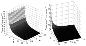
Figure 7: Arithmetic complexity percentile ratios (proposed versus conventional) for GEMM and CONV (frequency-domain) kernels of size $N$ using projection size $L$ and performing a single projection.

IV Experimental Results

We present results using the dual-core ARM Cortex A15 out-of-order superscalar processor (ARM v7 instruction set, bare metal, only one core was used and the other was powered down) with 32 KB L1 cache (for instructions and data) and 4 MB L2 cache. This processor has recently been integrated in popular System-on-Chip products marketed for multimedia applications in smartphone and home entertainment environments, such as Samsung’s Exynox 5, Exynox 5 Octa, Apple TV and the Google Chromebook portable computer. Similar results using our method were also obtained in an Intel Core i7-4700MQ 2.40GHz processor, but are omitted for brevity of exposition and also because energy consumption could not be measured as accurately as for the ARM processor based on the hardware available to us at the time of this writing.

The GEMM and CONV kernels were deployed on the ARM Cortex A15 using C code with 32-bit floating-point Neon instructions (ARM SIMD extensions utilizing the q registers of the processor) for accelerated processing. All codes were compiled by the ARM Development Studio 5 (DS5) C compiler under full optimization. Results were obtained using the ARM Versatile Express board with the V2P-CA15 (ASIC A15 chip) daughter-board and the ARM RealView ICE debugger unit. Dynamic and static power consumption was measured directly in hardware by the ARM energy probe. The board allows for dynamic voltage/frequency scaling (DVFS) between $V_{\text{dd}}=0.6$ V at $0.6$ GHz and $V_{\text{dd}}=0.85$ V at $1.2$ GHz at room temperature. In order to increase the reliability of our results, each experiment was performed 100 times using representative input data from image and audio streams normalized between $\left[-1,1\right]$; the presented precision–energy–throughput results stem from averages over all runs. Precision is measured in terms of SNR (dB) against the result computed by the conventional GEMM and CONV kernels in single-precision floating point. Energy is measured in milli-Joules (mJ) required for the completion of each task. Finally, throughput is measured in Mega-samples of results produced per second (MSamples/sec) by each kernel.

IV-A Resource–Precision Performance of GEMM and CONV kernels

Considering GEMM, out of several sets of experiments performed, we present results for subblocks with outer dimension of $N=144$, which corresponds to (or is a multiple of) the setting of other GEMM subblock kernels (e.g., Eigen, Goto BLAS [40] and throughput–precision GEMM scaling based on companding and packing [39]). We then selected two sizes for the inner dimension of GEMM: $40$ (leading to $144\times 40$ by $40\times 144$ GEMM subblocks) and $144$ (leading to $144\times 144$ by $144\times 144$ GEMM subblocks), which represent different operational complexities for the GEMM subblock realization. Finally, we utilized $L=8$ projections with coefficients derived via the DCT-II coefficient matrix of (7).

Figure 8–Figure 12 present results for precision–energy–throughput scaling against the conventional GEMM kernel realization, i.e. our SIMD-based GEMM kernel without projections. Two voltage and frequency levels are used and, as an external benchmark, we also present results with the Eigen GEMM kernel.

When using six projections (out of eight), the average SNR is $70$dB against the conventional GEMM kernel. Under the utilized input range and GEMM inner dimension, this corresponds to mean square error less than $7\times 10^{-4}$ in the GEMM results, which is deemed acceptable by all multimedia signal processing applications. This comes at no overhead in both throughput (in MSamples/sec) and energy consumption in comparison to the conventional GEMM kernel.

By reducing the number of projections, our approach achieves up to $85\%$ reduction in energy consumption against the conventional GEMM kernel (Figure 9 and Figure 10). This substantial reduction is energy comes from the reduction of execution time while maintaining the same level of power usage. More specifically, the power usage is identical during the GEMM inner-kenel computation and only increases by about 5% during the short time interval required to perform the projection. However, the projection process allows for the processing throughput to increase by $315\%\sim 533\%$ (Figure 11 and Figure 12, marginally less improvement is obtained against Eigen GEMM). These very substantial performance improvements come at the cost of decreasing the SNR to approximately $46\sim 65$ dB in comparison to the result computed under the conventional realization. We shall show in the next section that such SNR values offer sufficient accuracy for real-world multimedia recognition and matching systems utilizing GEMM computations.

As a final comparison, we evaluated these performance results against results obtained via throughput–precision GEMM based on our prior work on companding and packing [39]. On the same hardware platform, benchmarking the proposed approach under one projection against companding and packing GEMM led to: (i) more than $8$ dB gain in SNR; (ii) more than $60\%$ reduction of energy consumption; and (iii) more than $400$% increase of throughput. In conjunction with the fact that any number of projections can be deployed and that one is free to select projection coefficients suitable to the input data characteristics, this makes the proposed approach attain significantly broader resource–precision scalability in comparison to our previously-proposed companding-and-packing based GEMM.

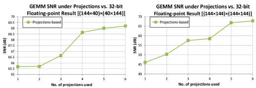
Figure 8: Precision for small and medium-size GEMM inner-dimension (left and right, respectively).

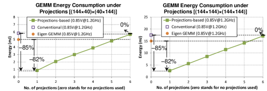
Figure 9: Energy-throughput results for small and medium-size GEMM inner-dimension (left and right, respectively) under high voltage and high frequency settings. “Conventional” refers to our conventional GEMM realization that does not utilize projections and it is used as a benchmark.

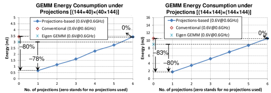
Figure 10: Energy-throughput results for small and medium-size GEMM inner-dimension (left and right, respectively) under low voltage and low frequency settings. “Conventional” refers to our conventional GEMM realization that does not utilize projections and it is used as a benchmark.

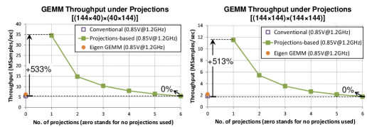
Figure 11: Throughput results for small and medium-size GEMM inner-dimension (left and right, respectively) under high voltage and high frequency settings. “Conventional” refers to our conventional GEMM realization that does not utilize projections and it is used as a benchmark.

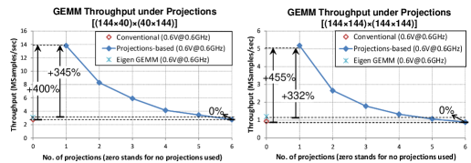
Figure 12: Throughput results for small and medium-size GEMM inner-dimension (left and right, respectively) under low voltage and low frequency settings. “Conventional” refers to our conventional GEMM realization that does not utilize projections and it is used as a benchmark.

Concerning the CONV kernel, we experimented with: block size of $W=20000$ samples, several kernel sizes between $N\in\left[600,1200\right]$ samples, $L=2$ projections using the Haar decomposition coefficients [43] and producing one projection at half sampling rate (and interpolating the missing samples) or one projection at full sampling rate. Representative precision–energy–throughput results with two settings for the kernel size are given in Tables II. We also present comparisons with convolution based on packed processing [44], as well as the equivalent results obtained by the conventional realization of our own SIMD-based CONV kernel (i.e. without projections) and the CONV kernel of the Cortex-A DSP library commercialized for ARM Neon by DSP Concepts LLC. The high energy consumption and low throughput reported in Table II for all approaches is due to the large block size used ($20000$ samples). The results demonstrate that the proposed approach substantially outperforms packed processing in terms of energy and throughput efficiency, while allowing for significantly higher SNR. Moreover, it allows for $82\%\sim 84\%$ reduction of energy consumption and $360\%\sim 400\%$ increase of processing throughput against the conventional CONV realization. Finally, while the SNR values of the proposed PET scaling within CONV remain significantly smaller than the ones of the conventional CONV kernel, it will be shown in the next section that this does not affect the accuracy of a real-world application performing audio matching based on cross-correlation.

Table II: Precision, energy and throughput scaling for CONV for two voltage and frequency levels. The results correspond to average SNR (in dB) over several inputs, with each SNR value measured against the equivalent result computed via the conventional CONV kernel.

Method	Precision		Energy (mJ)				Throughput (MSamples/sec)
	(dB)		$0.85$V@$1.2$GHz		$0.6$V@$0.6$GHz		$0.85$V@$1.2$GHz		$0.6$V@$0.6$GHz
Kernel size	$600$	$1200$	$600$	$1200$	$600$	$1200$	$600$	$1200$	$600$	$1200$
1 projection, half samples	19.82	22.87	596	1315	429	771	0.058	0.027	0.027	0.014
1 projection, all samples	20.07	23.41	1258	2366	826	1580	0.027	0.014	0.014	0.007
Packed processing [44]	17.65	13.60	1235	2556	850	1615	0.044	0.013	0.021	0.011
Conventional CONV	$\infty$	$\infty$	2476	4884	1654	3243	0.013	0.007	0.007	0.003
Cortex-A DSP CONV	141.47	143.33	2142	4005	1455	2692	0.016	0.008	0.008	0.004

V Resource–Precision Results within Error-tolerant Multimedia Recognition and Matching Applications

The proposed approach can bring important benefits to high-performance multimedia signal processing systems when the precision of computation is not of critical importance (error-tolerant systems), or when the input dataset is intrinsically noisy. This is quite common in image, video or audio analysis, recognition or matching applications, where the multimedia samples are contaminated with noise stemming from camera or microphone sensors or lossy coding systems [1]. Here, we present two representative applications for the proposed framework within two well-known image and audio recognition and matching systems proposed in the literature. While each of the two systems is deployed for a specific task (i.e. face recognition and music identification), the underlying algorithms are generic and can be applied to a wide variety of object recognition and audio matching tasks.

V-A Resource–Precision Trade-off in Face Recognition based on Principal Component Analysis (PCA)

State-of-the-art techniques for object recognition systems derive feature matrices and use 2D decomposition schemes via matrix multiplication in order to match features between a new image and an existing database of images (e.g. for automatic identification of human faces [9]). When such deployments run on embedded devices such as smartphones or smart visual sensors for image analysis and recognition [46], it is expected that thousands of training and recognition tasks should be computed with the highest-possible resource–precision capability of each core in order to minimize the required energy consumption and maximize the processing throughput.

Using the proposed approach, one can accelerate the real-time training and matching process for such applications. Specifically, the accelerated GEMM via projections can be used for the image covariance scatter matrix calculation during the training stage, as well as for the feature extraction from test input images [9]. In the following, we provide details of such a deployment for the prominent 2D-PCA system of Yang et al [9], which is widely regarded as one of the best-performing object recognition algorithms based on principal components.

The 2D-PCA algorithm for face recognition comprises three stages: training, feature extraction and matching. The training stage uses a number of training input images of human subjects and first calculates the image covariance scatter matrix from $J_{\text{set}}$ zero-mean input images, $\mathbf{A}_{j}$, by:

$$\mathbf{G}_{j}=\sum_{j=0}^{J_{\text{set}}-1}\mathbf{A}_{j}\mathbf{A}_{j}^{\text{T}}.$$ (22)

Based on this input training set, it then calculates the projection matrix comprising a series of projection axes (eigenvectors),

$$\mathbf{X}=\left[\left.\mathbf{x}_{0}\right|\left.\ldots\right|\mathbf{x}_{D-1}\right],$$ (23)

with $\mathbf{x}_{i}$, $0\leq i<D$ the orthonormal eigenvectors of $\mathbf{G}_{j}$ corresponding to its $D$ largest eigenvalues [9]. Each training-set image is mapped to $\mathbf{X}$ via:

$$\mathbf{Y}_{\text{set},j}=\mathbf{A}_{j}\mathbf{X}.$$ (24)

For the feature extraction stage, each new input image, $\mathbf{B}_{i}$ (test image), is mapped to $\mathbf{X}$ via:

$$\mathbf{Y}_{\text{test},i}=\mathbf{B}_{i}\mathbf{X},$$ (25)

with $\mathbf{Y}_{\text{test},i}$ comprising the feature matrix of test image $\mathbf{B}_{i}$. Finally, the matching stage determines for each test image the training-set image, $\mathbf{A}_{j_{\mathbf{B}_{i}}^{*}}$, with the smallest distance in their feature matrices:

$$j_{\mathbf{B}_{i}}^{*}=\arg\min_{\forall j}\left\|\mathbf{Y}_{\text{test},i}-\mathbf{Y}_{\text{set},j}\right\|_{F}.$$ (26)

The complexity of 2D-PCA is predominantly in the matrix multiplications required for the construction of $\mathbf{G}_{J}$ of (22) during the training stage and the mapping during the feature extraction, i.e. $\mathbf{Y}_{\text{test},i}$ of (25), as the eigenvalue decomposition required for the creation of $\mathbf{X}$ is only performed once every $J_{\text{set}}$ training images and very fast algorithms exist for the quick estimation of $j_{\mathbf{B}_{i}}^{*}$ of (26), such as the matching error measures of Lin and Tai [47].

To examine the impact of projections-based resource–precision scaling of GEMM, we utilize the proposed approach for all the matrix multiplication operations of (22), (24) and (25) of 2D-PCA. The Yale-A and Yale-B databases of face images (http://www.face-rec.org/databases/http://www.face-rec.org/databases/) were used for our experiments and, following prior work [9], each image was cropped to $288\times 288$ pixels (that includes the face portion) and the mean value was subtracted prior to processing.

Results from performing all matrix multiplication operations of (22), (24) and (25) with just one out of $L\in\left\{8,12,16\right\}$ projections [via the DCT-II coefficients of (7)] are presented in Table III for both Yale databases. Following [9], the first five images of each of the persons in each database were used for the training set and the remaining images per person were used as test images and we set $D=10$.

Starting with the case of $L=8$ projections, the table demonstrates that, for all GEMM computations, and under the same recognition accuracy as the conventional (non projections-based) GEMM, the proposed approach offers $440\%$ increase in the processing throughput and more than $80\%$ decrease in energy consumption. If we consider all the other operations and overheads of the entire face recognition application, the proposed approach still offers $350\%$ increase in the processing throughput and $79\%$ decrease in overall energy consumption. Importantly, we obtain the results of Table III based on two standard test image libraries (Yale-A and Yale-B databases of face images) and without any algorithmic modification. Instead, only a simple adjustment of the number of retained projections in the GEMM computations is required. This is a remarkably straightforward process compared to the previously-proposed packed processing [39] that requires resource–precision optimization amongst the subblock matrix products in order to provide for sufficient precision within the GEMM operations.

Furthermore, for $L=12$ and $L=16$ projections, Table III demonstrates that the energy and throughput scaling becomes even more substantial. Namely, between $672\%\sim 850\%$ of increase in throughput and $88\%\sim 91\%$ decrease in energy consumption is obtained against the conventional GEMM realization, with similar scaling when considering the entire application. However, these cases incur loss of recognition accuracy in the application in comparison to the conventional (non projections-based) GEMM. While this loss of recognition rate appears to be relatively limited, it can be undesirable in cases where maximizing the expected recognition rate is of paramount importance. We therefore conclude that the case of $L=8$ comprises an agreeable operational point, where substantial performance scaling is offered without any discernible impact in the application results.

Given the large performance increase, the lack of apparent degradation in the average recognition accuracy on both databases can be viewed as a non-intuitive result. However, this can be explained by the energy compaction performed by the algorithm itself. Essentially, the projection compacts the vast majority of the energy of the input images into one eighth of the data samples (using DCT coefficients) before performing the matrix product. Since all feature extraction and feature matching algorithms perform energy compaction anyway (from a large set of pixels to a few eigenvectors using PCA) in order to remove noise and retain only the principal components of each image covariance scatter matrix, the projections-based compaction during the GEMM kernel execution has limited or no effect on the average recognition accuracy of the system.

More broadly, the usage of energy compaction techniques is one of the primary reasons that error-tolerant multimedia signal analysis, matching and retrieval systems are known to be robust to noise in their inputs or intermediate computations [39, 48, 49, 1]. For instance, concerning multimedia retrieval systems in particular, the survey of Datta et al [48] points to various high-level analysis and retrieval systems that are robust to noise in the input data or in the calculated low-level feature points used for matching and retrieval processes (e.g. corner and edge points in images). Furthermore, well known studies have already analyzed the resilience of low-level feature extraction to noise [50] and recent work [51, 52, 11] has indicated significant complexity-precision tradeoffs in feature extraction algorithms by incremental or approximate computation of their computationally-intensive kernels (transforms, distance metric calculations, matrix-vector products) in space or frequency domain. Finally, learning algorithms for large data sets have traditionally been known to be robust to noise in the input or processed data [49]. However, as explained in the introduction section, exploiting the inherent energy compaction properties of error-tolerant multimedia signal processing and analysis algorithms has only achieved limited performance scaling in programmable processors [1, 35, 44] because, until now, only hardware-oriented approaches [15, 53, 54, 55, 56, 25, 37, 29, 30] could scale the precision of computations and achieve significant energy or throughput scaling.

Table III: Recognition percentage vs. energy–throughput results for GEMM computations within the 2D-PCA algorithm for face recognition. All results were produced with $V_{\text{dd}}=0.6$V at $0.6$GHz.

Method	Recognition rate ($\%$)	Recognition rate ($\%$)	Energy per match	Throughput per match
	for Yale-A database	for Yale-B database	(mJ)	(MSamples/sec)
Proposed	78.40	86.59	29.99	1.24
projections-based
GEMM, $L=8$
Proposed	76.81	83.16	21.42	1.75
projections-based
GEMM, $L=12$
Proposed	74.22	80.31	16.44	2.15
projections-based
GEMM, $L=16$
Conventional GEMM	78.40	86.59	174.79	0.23
Packing-based	78.81	86.59	99.58	0.39
GEMM [39]
Eigen GEMM	78.40	86.59	141.96	0.27

V-B Resource–Precision Trade-off in Feature Vector Cross-correlation within a Music Matching System

We selected as the second test case a recently-proposed music matching system that matches cover songs [12] with the songs available in an existing database. For each input song to be identified, the system works by extracting beat and tempo data and then matching it to the (precalculated) beat and tempo database via cross correlation. Matlab code for this and the sample data were collected from the authors’ site [12]. Given that this implementation is dominated by the cross-correlation operations [12], the only modification performed was the replacement of the Matlab xcorr() function call with our CONV kernel running on the ARM test-bed. Thus, in this case each input block of the cross-correlation corresponds to a song’s beat and tempo data and each convolution kernel comprises the beat and tempo data of a song of the database. The settings used for our experiments were: average beat rate 120 beats-per-minute, chroma element central frequency 200Hz [12].

Concerning our implementation, we utilized one out of $L\in\left\{2,4\right\}$ projections and used the Haar decomposition (and synthesis) coefficients. Table IV demonstrates that these settings yielded the same matching accuracy for all methods for $L=2$ projections ($53.75\%$ match), while providing up to $286\%$ increase in throughput (and $75\%$ decrease in energy consumption) in comparison to the conventional CONV implementation. The overall throughput increase for the entire music-matching application (i.e., including I/O overhead and the feature extraction from the original audio) is $273\%$ (and $72\%$ decrease in energy consumption). The competing acceleration mechanism, i.e., asymmetric companding-and-packing from our previous work [44], turns out to be significantly slower and less energy-efficient than the proposed approach.

Furthermore, for $L=4$ projections, the matching accuracy of the proposed approaches decreases ($47.21\%$ match), while providing for even more substantial throughput and energy scaling in comparison to the conventional CONV implementation, i.e., $569\%$ and $86\%$ respectively. Nevertheless, the small reduction of the matching accuracy may make this case undesirable to use in a practical deployment.

Similarly as for the case of face recognition, the proposed approach incurs no side effects in the matching accuracy of the system for $L=2$ projections as the utilized beat and tempo features are inherently noisy and the retained energy in the feature datasets after the projection suffices for equally-accurate matching over the test dataset.

Table IV: Matching accuracy vs. energy-throughput scaling for CONV (cross-correlation) computations per matching operation within a music identification application using beat and tempo features. All results were produced with $V_{\text{dd}}=0.6$V at $0.6$GHz.

Method	Matching ($\%$)	Energy (mJ)	Throughput
			(MSamples/sec)
Proposed	53.75	2122	0.027
projections-based
CONV, $L=2$
Proposed	47.21	1123	0.046
projections-based
CONV, $L=4$
Conventional	53.75	8254	0.007
CONV
Packing-based	53.75	4284	0.021
CONV [44]
Cortex-A DSP	53.75	7264	0.008
CONV

VI Conclusion

We propose an approach to systematically trade-off precision for substantial energy and throughput scaling in generic matrix multiplication (GEMM) and discrete convolution (CONV) kernels. Given that our approach applies linear projections within the top-level processing of these kernels, it allows for seamless scaling of resources versus the accuracy of the performed computations without cumbersome and algorithm- or application-specific customization. Experiments with the recently-introduced ARM Cortex A15 processor on a dedicated test-bed supporting different voltage and frequency levels and accurate energy measurement, demonstrate that our proposal leads to more than five-fold reduction of energy consumption and more than five-fold increase of processing throughput against the conventional (i.e., non projections-based) realization of GEMM and CONV kernels. Experimental results within multimedia recognition and matching applications show that the precision loss incurred by the proposed projections-based GEMM and CONV kernels can be tolerated with limited or no noticeable effect on the recognition and matching accuracy of applications and that our proposal allows for truly dynamic adaptation without incurring reconfiguration overheads.

The proposed approach opens up a new avenue for dynamic precision–energy–throughput scaling within high-performance GEMM and CONV kernel designs. For the first time, linear transforms can be used towards dynamic resource scaling of such kernels with graceful precision degradation. Even though in this paper we used well-known non-adaptive transforms for the projection coefficients, such as the discrete cosine transform and the Haar transform, if training input datasets are available a-priori, projections based on principal component analysis could be employed (with their coefficients derived offline) for optimized precision–energy–throughput scaling within each error-tolerant multimedia application. Alternatively, if feedback on the incurred imprecision in the results is available via the application, the projection mechanism of the GEMM and CONV kernels can be tuned to learn the best projection parameters. These are aspects that can be explored in future work.

References

- [1] Y. Andreopoulos, “Error tolerant multimedia stream processing: There’s plenty of room at the top (of the system stack),” IEEE Trans. on Multimedia, vol. 15, no. 2, pp. 291–303, Feb. 2013.
- [2] B.K. Khailany, T. Williams, J. Lin, E.P. Long, M. Rygh, D.F.W. Tovey, and W.J. Dally, “A programmable 512 gops stream processor for signal, image, and video processing,” IEEE J. Solid-State Circ., vol. 43, no. 1, pp. 202–213, Jan. 2008.
- [3] J. Ostermann, J. Bormans, P. List, D. Marpe, M. Narroschke, F. Pereira, T. Stockhammer, and T. Wedi, “Video coding with h. 264/avc: tools, performance, and complexity,” IEEE Circ. and Syst. Mag., vol. 4, no. 1, pp. 7–28, Jan. 2004.
- [4] T.Y. Yeh, G. Reinman, S.J. Patel, and P. Faloutsos, “Fool me twice: Exploring and exploiting error tolerance in physics-based animation,” ACM Trans. on Graphics, vol. 29, no. 1, article 5, Jan. 2009.
- [5] T. Kim and D.L. James, “Skipping steps in deformable simulation with online model reduction,” ACM Trans. on Graphics, vol. 28, no. 5, article 123, 2009.
- [6] Z. Zhu, I. Cox, and M. Levene, “Ranked-listed or categorized results in ir: 2 is better than 1,” Proc. Internat. Conf. Nat. Lang. and Inf. Systems, NLDB’08, pp. 111–123, 2008.
- [7] K. Petridis, D. Anastasopoulos, C. Saathoff, N. Timmermann, Y. Kompatsiaris, and S. Staab, “M-ontomat-annotizer: Image annotation linking ontologies and multimedia low-level features,” in Proc. Knowledge-Based Intell. Inf. and Eng. Syst. (LNCS-4253), 2006, pp. 633–640.
- [8] R.A. Newcombe, S. Izadi, O. Hilliges, D. Molyneaux, D. Kim, A.J. Davison, P. Kohli, J. Shotton, S. Hodges, and A. Fitzgibbon, “KinectFusion: Real-time dense surface mapping and tracking,” in Proc. 10th Symp. Mixed and Augm. Real., ISMAR’11, 2011, pp. 127–136.
- [9] J. Yang, D. Zhang, A.F. Frangi, and J. Yang, “Two-dimensional PCA: a new approach to appearance-based face representation and recognition,” IEEE Trans. on Pat. Anal. and Mach. Intel., vol. 26, no. 1, pp. 131–137, Jan. 2004.
- [10] B. Foo and M. van der Schaar, “A distributed approach for optimizing cascaded classifier topologies in real-time stream mining systems,” IEEE Trans. on Image Process., vol. 19, no. 11, pp. 3035–3048, Nov. 2010.
- [11] P. Mainali, Q. Yang, G. Lafruit, L. Gool, and R. Lauwereins, “Robust low complexity corner detector,” IEEE Trans. on Circ. and Syst. for Video Technol., vol. 21, no. 4, pp. 435–445, Apr. 2011.
- [12] D.P.W. Ellis, C.V. Cotton, and M.I. Mandel, “Cross-correlation of beat-synchronous representations for music similarity,” in Proc. IEEE Int. Conf. on Acoust., Speech and Signal Process., ICASSP’08, 2008, pp. 57–60.
- [13] R. Kannan P. Drineas and M.W. Mahoney, “Fast monte carlo algorithms for matrices i: Approximating matrix multiplication,” SIAM J. Comput, vol. 36, no. 1, pp. 132–157, May 2006.
- [14] J.T. Ludwig, S.H. Nawab, and A.P. Chandrakasan, “Low-power digital filtering using approximate processing,” IEEE J. Solid-State Circ., vol. 31, no. 3, pp. 395–400, Mar. 1996.
- [15] N.R. Shanbhag, R.A. Abdallah, R. Kumar, and D.L. Jones, “Stochastic computation,” in Proc. Design, Automat. & Test in Europe Conf. & Expo., DATE’10, 2010, pp. 859–864.
- [16] N. Merhav and R. Kresch, “Approximate convolution using dct coefficient multipliers,” IEEE Tran. On Circuits and Systems for Video Technology, vol. 8, no. 4, pp. 378–385, Aug. 1998.
- [17] Y. Chen and H. Sundaram, “Basis projection for linear transform approximation in real-time applications,” in Proc. IEEE Int. Conf. Acoust., Speech and Signal Process., ICASSP’06, 2006, vol. 2, pp. II–II.
- [18] L. Di Stefano and S. Mattoccia, “Fast template matching using bounded partial correlation,” J. Machine Vision and Applications, vol. 13, no. 4, pp. 213–221, Feb. 2003.
- [19] A. Kadyrov and M. Petrou, “The Invaders’ algorithm: range of values modulation for accelerated correlation,” IEEE Trans. on Pat. Anal. and Mach. Intel., vol. 28, no. 11, pp. 1882–1886, Nov. 2006.
- [20] D. Anastasia and Y. Andreopoulos, “Linear image processing operations with operational tight packing,” IEEE Signal Process. Lett., vol. 17, no. 4, pp. 375–378, Apr. 2010.
- [21] H. Chung and A. Ortega, “Analysis and testing for error tolerant motion estimation,” in Proc. 20th IEEE Int. Symp. on Defect and Fault Tol. in VLSI Syst., DFT’05, 2005, pp. 514–522.
- [22] K. Lengwehasatit and A. Ortega, “Scalable variable complexity approximate forward dct,” IEEE Circ. and Syst. for Video Technol., vol. 14, no. 11, pp. 1236–1248, Nov. 2004.
- [23] K. Lee, A. Shrivastava, N. Dutt, and N. Venkatasubramanian, “Cc-protect: Cooperative cross-layer protection to mitigate the impact of hardware defects on multimedia applications,” ACM Trans. on Computat. Logic, submitted.
- [24] J. Sartori and R. Kumar, “Branch and data herding: Reducing control and memory divergence for error-tolerant gpu applications,” IEEE Trans. on Multimedia, vol. 15, no. 2, pp. 279–290, Feb. 2013.
- [25] R. A. Abdallah and N. R. Shanbhag, “Robust and energy efficient multimedia systems via likelihood processing,” IEEE Trans. on Multimedia, vol. 15, no. 2, pp. 257–267, Feb. 2013.
- [26] T. Austin, D. Blaauw, T. Mudge, and K. Flautner, “Making typical silicon matter with razor,” IEEE Comput., vol. 37, no. 3, pp. 57–65, Mar. 2004.
- [27] W. Qian, X. Li, M.D. Riedel, K. Bazargan, and D.J. Lilja, “An architecture for fault-tolerant computation with stochastic logic,” IEEE Trans. on Comput, vol. 60, no. 1, pp. 93–105, Jan. 2011.
- [28] A. Lingamneni, K.K. Muntimadugu, C. Enz, R.M. Karp, K.V. Palem, and C. Piguet, “Algorithmic methodologies for ultra-efficient inexact architectures for sustaining technology scaling,” in Proc. 9th ACM Conf. Comput. Front., 2012, pp. 3–12.
- [29] P.N. Whatmough, S. Das, D.M. Bull, and I. Darwazeh, “Circuit-level timing error tolerance for low-power dsp filters and transforms,” IEEE Trans. on Very Large Scale Integr. (VLSI) Syst., vol. 21, no. 6, pp. 989–999, 2013.
- [30] P.N. Whatmough, S. Das, D.M. Bull, and I. Darwazeh, “Selective time borrowing for dsp pipelines with hybrid voltage control loop,” in 2012 17th Asia and South Pacific Design Automation Conference (ASP-DAC), 2012, pp. 763–768.
- [31] R. E. Blahut, Fast algorithms for signal processing, Cambridge University Press, Cambridge, UK, 2010.
- [32] A. Skodras, “Fast discrete cosine transform pruning., vol. 42, no. 7, pp. , july 1994.,” IEEE Trans. on Signal Process, vol. 42, no. 7, pp. 1833–1837, Jul. 1994.
- [33] K-I Kum S. Kim and W. Sung, “Fixed-point optimization utility for c and c++ based digital signal processing programs, vol. 45, no. 11, pp. , nov. 1998.,” IEEE Trans. Circ. and Syst.-II, vol. 45, no. 11, pp. 1455–1464, Nov. 1998.
- [34] R. Yuster and U. Zwick, “Fast sparse matrix multiplication,” ACM Trans. on Algorithms, vol. 1, no. 1, Jul. 2005.
- [35] D. Anastasia and Y. Andreopoulos, “Software designs of image processing tasks with incremental refinement of computation,” IEEE Trans. Image Process., vol. 19, no. 8, pp. 2099–2114, Aug. 2010.
- [36] A.P. Chandrakasan J.M. Winograd S.H. Nawab, A.V. Oppenheim and J.T. Ludwig, “Approximate signal processing,” J. of VLSI Signal Process, vol. 15, no. 1, Jan. 1997.
- [37] D.L. Jones S. Narayanan, G.V. Varatkar and N.R. Shanbhag, “Computation as estimation: A general framework for robustness and energy efficiency in socs,” IEEE Trans. on Signal Process., vol. 58, no. 8, pp. 4416–4421, Aug. 2010.
- [38] D.G. Murray and S. Hand, “Spread-spectrum computation,” in Proc. 4th USENIX Conf. on Hot Top. in Syst. Depend., 2008, pp. 5–8.
- [39] D. Anastasia and Y. Andreopoulos, “Throughput-distortion computation of generic matrix multiplication: Toward a computation channel for digital signal processing systems,” IEEE Trans. on Signal Process., vol. 60, no. 4, pp. 2024–2037, Apr. 2011.
- [40] K. Goto and R. Van De Geijn, “High-performance implementation of the level-3 blas,” ACM Trans. on Math. Soft., vol. 35, no. 1, article 4, Jan. 2008.
- [41] E. Agullo, J. Demmel, J. Dongarra, B. Hadri, J. Kurzak, J. Langou, H. Ltaief, P. Luszczek, and S. Tomov, “Numerical linear algebra on emerging architectures: The PLASMA and MAGMA projects,” in J. of Phys.: Conference Series, 2009, vol. 180, no 012037.
- [42] Z. Chen and J. Dongarra, “Algorithm-based checkpoint-free fault tolerance for parallel matrix computations on volatile resources,” in Proc. 20th Int. Par. and Distr. Process. Symp., IPDPS’06. IEEE, 2006, pp. 10–15.
- [43] A. V Oppenheim, R. W Schafer, J. R Buck, et al., Discrete-time signal processing, vol. 5, Prentice hall Upper Saddle River, 1999.
- [44] M.A. Anam and Y. Andreopoulos, “Throughput scaling of convolution for error-tolerant multimedia applications,” IEEE Trans. on Multimedia, vol. 14, no. 2, pp. 797–804, Jun. 2012.
- [45] F. Franchetti, M. Puschel, Y. Voronenko, S. Chellappa, and J. Moura, “Discrete fourier transform on multicore,” IEEE Signal Process. Mag., vol. 26, no. 6, pp. 90–102, 2009.
- [46] B. Kisačanin, S. S Bhattacharya, and S. Chai, Embedded computer vision, Springerverlag London Limited, 2009.
- [47] Y.-C. Lin and S.-C. Tai, “Fast full-search block-matching algorithm for motion-compensated video compression,” IEEE Trans. on Commun., vol. 45, no. 5, pp. 527–531, 1997.
- [48] R. Datta, D. Joshi, J. Li, and J.Z. Wang, “Image retrieval: Ideas, influences, and trends of the new age,” ACM Computing Surveys, vol. 40, no. 2, pp. 5, Apr. 2008.
- [49] Keinosuke Fukunaga, Introduction to statistical pattern recognition, Elsevier Acad. Press, ISBN 0122698517, 1990.
- [50] C. Schmid, R. Mohr, and C. Bauckhage, “Evaluation of interest point detectors,” Int. J. of Comp. Vis., vol. 37, no. 2, pp. 151–172, Feb. 2000.
- [51] Y. Andreopoulos and I. Patras, “Incremental refinement of image salient-point detection,” IEEE Trans. on Image Process, vol. 17, no. 9, pp. 1685–1699, Sept. 2008.
- [52] D.M. Jun and D.L. Jones, “An energy-aware framework for cascaded detection algorithms,” in IEEE Worksh. on Signal Process. Syst., SIPS’10, 2010, pp. 1–6.
- [53] S. Narayanan, J. Sartori, R. Kumar, and D.L. Jones, “Scalable stochastic processors,” in Proc. Design, Automat. & Test in Europe Conf. & Expo., DATE’10, 2010, pp. 335–338.
- [54] P. Korkmaz, B.E.S. Akgul, and K.V. Palem, “Energy, performance, and probability tradeoffs for energy-efficient probabilistic cmos circuits,” IEEE Trans. Circ. and Syst. I: Reg. Papers, vol. 55, no. 8, pp. 2249–2262, Aug. 2008.
- [55] P. Subramanyan, V. Singh, K.K. Saluja, and E. Larsson, “Multiplexed redundant execution: A technique for efficient fault tolerance in chip multiprocessors,” in Proc. Des., Autom. & Test in Europe Conf. & Expo., DATE’10, 2010, pp. 1572–1577.
- [56] L. Leem, H. Cho, J. Bau, Q.A. Jacobson, and S. Mitra, “ERSA: Error resilient system architecture for probabilistic applications,” in Proc. Des., Autom. & Test in Europe Conf. & Expo., DATE’10, 2010, pp. 1560–1565.