Level spacing distribution
for the prototype of the Bianchi IX model††thanks: Presented
at the conference Random Matrix Theory: Foundations and Applications, Kraków, July 1-6, 2014.
Abstract
Our results concern quantum chaos of the vacuum Bianchi IX model. We apply the equilateral triangle potential well approximation to the potential of the Bianchi IX model to solve the eigenvalue problem for the physical Hamiltonian. Such approximation is well satisfied in vicinity of the cosmic singularity. Level spacing distribution of the eigenvalues is studied with and without applying the unfolding procedure. In both cases, the obtained distributions are qualitatively described by Brody’s distribution with the parameter , revealing some sort of the level repulsion. The observed repulsion may reflect chaotic nature of the classical dynamics of the Bianchi IX universe. However, full understanding of this effects will require examination of the Bianchi IX model with the exact potential.
05.45.Mt, 98.80.Qc
1 Introduction
Astronomical observations tell us that the Universe has been expanding for almost 14 billion years so it must have emerged from a state with extremely high energy densities of matter fields. Theoretical attempts of understanding the early stage of the Universe are, however, plagued by the cosmological singularity characterized by blowing up of physical invariants. This concerns almost all known general relativity models of the universe (Friedmann, Lemaître, Kasner, Bianchi, Szekeres, …). The existence of the cosmological singularities in solutions to Einstein’s equations means that this classical theory is incomplete. Expectation is that quantization may heal the singularities.
The Friedmann-Robertson-Walker (FRW) model, which is homogenous and isotropic, is commonly used to describe the cosmological data. However, the isotropy is dynamically unstable in the backward evolution towards the cosmic singularity [1]. The general anisotropic model including FRW as a special case is the Bianchi IX model. It is the best prototype for the Belinskii, Khalatnikov and Lifshitz (BKL) scenario, which is thought to be a generic solution to the Einstein equations near the cosmological singularity [2, 3].
The classical dynamics of the Bianchi IX model is both singular [2, 4] and chaotic [2, 4, 5]. In this article we look for symptoms of the chaotic behavior at the quantum level. For this purpose, the spectrum of canonically quantized Hamiltonian for the vacuum Bianchi IX model is analyzed. In our considerations, the hard wall approximation (which is well satisfied in vicinity of the cosmic singularity) for the Bianchi IX potential is applied.
2 The Bianchi IX model
The Bianchi IX model can be viewed as a generalization of the positively curved () FRW with two additional degrees of freedom parameterizing the anisotropy [6]. The line element of the model reads
| (1) |
where are 1-forms satisfying . The is a lapse function and the function are usually parametrised as , where . The is an average scale factor related to , playing a role of internal time. Based on the functions, it is convenient to define parameters and . The closed () FRW model is recovered for , with corresponding to the FRW scale factor.
The action integral for Bianchi type models reads [4, 7]
| (2) |
where and are canonical variables, , whereas is the physical (true) Hamiltonian. The relation of the internal time to the cosmic time reads: [7].
The Hamiltonian in (2) has the form
| (3) |
where the potential for the Bianchi IX model is defined to be
| (4) |
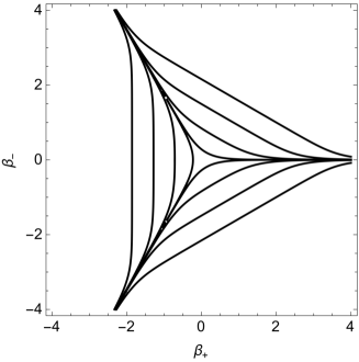
As seen from Fig. 1, the potential is characterized by symmetry with equipotential lines asymptotically arranging in the form of the equilateral triangle.

3 Quantization
In order to quantize the system, the canonical procedure of quantization is applied:
| (5) |
Using the Schorödinger representation for the above commutation relation, the quantum operator corresponding to (3) reads:
| (6) |
The domain is chosen in such a way that the operator is self-adjoint, where with the subset defined as:
| (7) |
The eigenproblem for the is equivalent to solving the Schrödinger equation for a particle in two dimensional potential well. The difficulty in solving this equation is due to complicated form of the potential, which would require application of sophisticated numerical techniques. However, near the singularity (when ), the potential can be approximated by the hard walls equilateral triangle potential [4, 8]. This can be deduced from the structure of the equipotential lines of (see Fig. 1) as well as from the asymptotic form of the potential for . The effective triangle in which the motion takes place is found to be [4]: .
Employing the hard wall approximation, the operator given by (6) reduces to
| (8) |
with the domain
| (9) |
The Hilbert space has the inner product . One can show that the operator (8) defined on (9) is self-adjoint. Thus, the eigenvalues of the operator are real and the corresponding eigenvectors form an orthogonal set. Despite of non-separability, the eigenequation can be solved analytically, leading to the following set of eigenvalues [9]:
| (10) |
where , and the eigenvalues are labeled by
| (11) |
and where
| (12) |
In what follows we are interested in the spectrum of the operator rather than the . Because of self-adjointness of the operator the spectrum of can be obtained from the spectral decomposition . The operator is positive . Thus, the spectrum of is real and given by (up to the overall sign):
| (13) |
4 Chaotic dynamics
The classical dynamics of the Bianchi IX model exhibits chaotic behavior (see, e.g. [5]), reflecting non-integrability of the system. The chaotic nature of the classical dynamics can be observed also at the quantum level. In particular, it has been shown that wave packets evolving in the Bianchi IX potential undergo defragmentation characterizing chaotic behavior [10, 11].
An alternative way of looking at chaoticity of the quantum systems is by analyzing spectra of the Hamiltonian operators. Namely, it has been conjectured that chaotic nature of the classical dynamics leads to the level repulsion in the quantum theory [12, 13]. This behavior can be characterized by different statistics of the level spacing variable, with the mean value normalized to unity.
In case of the non-integrable systems, the level spacing distribution is often characterized by the distribution obtained for Gaussian Orthogonal Ensemble (GOE) of the random matrices:
| (14) |
In contrast, integrable systems are characterized roughly by the Poisson distribution
| (15) |
In real system, chaotic and regular regimes often coexist: the level spacing distribution can be modeled by distribution interpolating between Poisson and GOE distributions, such as the Brody distribution
| (16) |
where . At the limits of the interval we have and .
5 Level spacing distribution
In this section, statistical properties of eigenvalues of the prototype of the Bianchi IX with the potential approximated by the hard wall equilateral triangle are analyzed. For this purpose degeneracy of the spectrum (13) has to be removed firstly. The different eigenvalues are subsequently sorted ascending () and the level-spacings are computed. Distribution of cannot be compared to the scale-free distributions (14) and (15). This requires introducing normalized level-spacing , defined such that the mean value . The simplest way is to rescale where . In Fig. 2 we present corresponding distributions for two different values of the number of eigenvalues and .
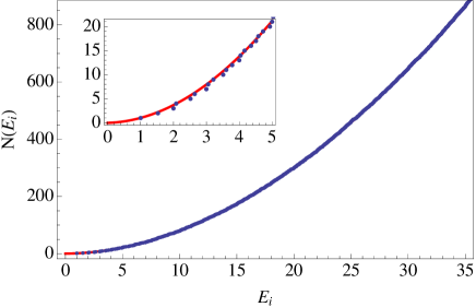
The spectrum of eigenvalues is usually inhomogeneous (averages over its different regions do not overlap). In order to extract information about the local correlations, global trend in the spectrum has to be subtracted. This can be performed by applying the so-called unfolding of the spectrum. In what follows we apply the procedure to the spectrum (13). For this purpose we define and (as previously) construct non-degenerate spectrum from it. Based on this, the function is defined such that . The function together with the polynomial fit
| (17) |
is shown in Fig. 3. The fit has been performed using the least-squares method for .

The fitted function allows us for the following decomposition , where quantifies fluctuations around the mean value. Now the new spectrum can be defined as . The advantage of such definition is that the corresponding distribution of level spacing is well normalized, because
| (18) |
Indeed, for the fit (17) performed for we obtain . In Fig. 4 we present distributions of the unfolded spectra for two different values of the number of eigenvalues and .
In this case fluctuation are greater than previously, therefore size of the bin has been increased to in order to smoothen the spectrum. Furthermore, for the unfolding procedure has been performed based on the new fit , which gives . The fit (17) performed for is no more valid for the case.
6 Summary
The level spacing distributions obtained with and without applying the unfolding procedure are qualitatively similar. This indicates that inhomogeneity of the spectrum does not play a significant role. Both spectra are qualitatively described by the Brody’s distribution with the parameter . The observed deficit of the small level spacing (with respect to the Poisson distribution) indicates for level repulsion, which might reflect chaotic nature of Bianchi IX model. Confirmation of this observation might be provided by the further analysis of fluctuations of the unfolded spectra [14]. Furthermore, next step would be numerical examination of the level statistics of the Bianchi IX with the exact potential.
Acknowledgments. W.P. would like to thank the organizers of the Conference for creating an inspiring atmosphere, and for financial support.
References
- [1] E. M. Lifshitz and I. M. Khalatnikov, Adv. Phys. 12 (1963) 185.
- [2] V. A. Belinsky, I. M. Khalatnikov, E. M. Lifshitz, Adv. Phys. 19 (1970) 525.
- [3] V. A. Belinsky, I. M. Khalatnikov, E. M. Lifshitz, Adv. Phys. 31 (1982) 639.
- [4] C. W. Misner, “Quantum Cosmology”, Phys. Rev. 186, 1319 (1969).
- [5] N. J. Cornish and J. J. Levin, Phys. Rev. Lett. 78 (1997) 998; Phys. Rev. D 55 (1997) 7489
- [6] D. H. King, Phys. Rev. D 44, 2356 (1991).
- [7] C. W. Misner, “Minisuperspace”, in Magic Without Magic: John Archibald Wheeler, p. 441, Ed. by J. R. Klauder (W.H. Freeman and Company, San Francisco, 1972).
- [8] M. P. Ryan Jr., and L. C. Sheply, Homogeneous Relativistic Cosmologies (Princeton University Press, Princeton, 1975).
- [9] Wai-Kee Li, S.M. Blinder, J. Math. Phys. 26, 2784 (1985).
- [10] T. Furusawa, Prog. Theor. Phys. 75 (1986) 59; 76 (1986) 67.
- [11] B. K. Berger, Phys. Rev. D 39 (1989) 2426.
- [12] O. Bohigas, M. J. Giannoni and C. Schmit, Phys. Rev. Lett. 52 (1984) 1.
- [13] F. Haake, Quantum Signatures of Chaos (Springer, Berlin, 2001).
- [14] A. Relano, J. M. G. Gomez, R. A. Molina, J. Retamosa, and E. Faleiro, Phys. Rev. Lett. 89, 244102 (2002).