Entropy and long-range correlations in DNA sequences

Abstract

We analyze the structure of DNA molecules of different organisms by using the additive Markov chain approach. Transforming nucleotide sequences into binary strings, we perform statistical analysis of the corresponding “texts”. We develop the theory of $N$-step additive binary stationary ergodic Markov chains and analyze their differential entropy. Supposing that the correlations are weak we express the conditional probability function of the chain by means of the pair correlation function and represent the entropy as a functional of the pair correlator. Since the model uses two point correlators instead of probability of block occurring, it makes possible to calculate the entropy of subsequences at much longer distances than with the use of the standard methods. We utilize the obtained analytical result for numerical evaluation of the entropy of coarse-grained DNA texts. We believe that the entropy study can be used for biological classification of living species.

I Introduction

At present there is a commonly accepted viewpoint that our world is complex and correlated. For this reason systems with long-range interactions (and/or with long-range memory) and natural sequences with non-trivial information content have been the focus of a large number of studies in different fields of science over the past several decades. Some of the most peculiar manifestations of this concept are DNA and protein sequences Buldyrev ; Almir ; mad .

One of the efficient methods to investigate the correlated systems is based on the decomposition of the space of states into a finite number of parts labeled by definite symbols. This procedure, referred to as a coarse graining, is accompanied by the loss of short-range memory between states of system but does not affect and does not damage its robust invariant statistical properties on large scales. The most frequently used method of the decomposition is based on the introduction of two parts of the phase space. In other words, it consists in mapping the two parts of states onto two symbols, say 0 and 1. Thus, the problem is reduced to investigating the statistical properties of the symbolic binary sequences. This method is applicable for the examination of both discrete and continuous systems Eren ; Lind .

There are many methods for describing the complex dynamical systems and random sequences connected with them: correlation function, fractal dimensions, multi-point probability distribution functions, and many others. One of the most convenient characteristics serving to the purpose of studying complex dynamics is the entropy Shan ; Cover . Being a measure of the information content and redundancy in a sequence of data it is a powerful and popular tool in examination of the complexity phenomena. It has been used for the analysis of a number of different dynamical systems.

A standard method of understanding and describing statistical properties of real physical systems or random sequences of data can be represented as follows. First of all, we need to analyze the sequence to find the correlation functions or the probabilities of words occurring, with the length $L$ exceeding the correlation length $R_{c}$ but being shorter than the length $M$ of the sequence,

$$R_{c}<L<<M.$$ (1)

At the same time, the number $d^{L}$ of different words of the length $L$ composed in the alphabet containing $d$ letters has to be much less than the number $M-L$ of words in the sequence,

$$d^{L}<<M.$$ (2)

The next step is to express the correlation properties of the sequence in terms of the conditional probability function (CPF) of the Markov chain, see below Eq. (5). Note, the Markov chain should be of order $N$, which is supposed to be longer than the correlation length,

$$R_{c}<N.$$ (3)

This is the critical requirement because the correlation length of natural sequence of interest (e.g., written or DNA texts) is usually of the same order as the length of sequences. None of inequalities (1)—(3) can be fulfilled. Really, the lengths of words that could represent correctly the probability of words occurring are 4-5 letters for a real natural text of the length $10^{6}$ (written on an alphabet containing 27-30 letters and symbols) or of order of 20 symbols for a coarse-grained text represented by means of a binary sequence.

So, it is clear that the method described above can only describe the random sequences with short correlation lengths and is not suited for analyzing the systems with long-range correlations. The latter issue will be the subject of our interest. We suppose that all we need for constructing the sequence with long-range correlations are the pair correlation functions.

We use the developed method muya for constructing the conditional probability function presented by means of the pair correlator which makes it possible to calculate analytically the entropy of the sequence. It should be stressed that we suppose that the correlations are weak but not short.

The scope of the paper is as follows. First, we discuss briefly $N$-step additive Markov chain model RewUAMM and, supposing that the correlations between symbols in the sequence are weak, we express the conditional probability function by means of the pair correlation function. In the next section we represent the differential entropy in terms of the conditional probability function of the Markov chain and express the entropy as the sum of squares of the pair correlators. Then we discuss some properties of the results obtained. Next, a fluctuation contribution to the entropy due to finiteness is examined. The application of the developed theory to some specific DNA sequences of nucleotides is considered. In conclusion, some remarks on directions in which the research can be progressed are presented.

II Additive Markov chains

Consider a sequence $\mathbb{A}=a_{-\infty}^{\infty}=...,a_{-1},a_{0},a_{1},...$ of real random variables $a_{i}$ taken from the finite alphabet $A=\{1,2,...,d\}$, $a_{i}\in A$. The sequence $\mathbb{A}$ is $N$-step Markov chain (also referred to as the higher-order or $N$-th-order Markov chain Raftery ; Ching ; Li ; Cocho ; Seifert ) if it possesses the following property: the probability of symbol $a_{i}$ to have a certain value $a$ under the condition that the values of all previous symbols are specified depends only on the values of $N$ previous symbols,

$$P(a_{i}=a|\ldots,a_{i-2},a_{i-1})$$ (4)

$$=P(a_{i}=a|a_{i-N},\ldots,a_{i-2},a_{i-1}).$$

Sometimes the number $N$ is also referred to as the memory length of the Markov chain. The conditional probability function (CPF) $P(a_{i}=a|a_{i-N},\ldots,a_{i-2},a_{i-1})$ determines completely all statistical properties of the Markov chain and the method of its iterative numerical construction. If the sequence, whose statistical properties we would like to analyze is assigned, the conditional probability function of the $N$-th order can be found by a standard method,

$$P(a_{N+1}=a|a_{1},\ldots,a_{N})=\frac{P(a_{1},\ldots,a_{N},a)}{P(a_{1},\ldots,a_{N})},$$ (5)

where $P(a_{1},\ldots,a_{N},a)$ and $P(a_{1},\ldots,a_{N})$ are the probabilities of the $(N+1)$-word $a_{1},\ldots,a_{N},a$ and $N$-word $a_{1},\ldots,a_{N}$ occurring, consequently.

The Markov chain determined by Eq. (4) is a homogeneous sequence because its conditional probability does not depend explicitly on $i$, i.e., is independent of the position of symbols $a_{i-N},\ldots,a_{i-1},a_{i}$ in the chain. It depends only on the values of $a_{i-N},\ldots,a_{i-1},a_{i}$ and their positional relationship. The homogeneous sequences are stationary: the average value of any function $f(a_{r_{1}},a_{r_{1}+r_{2}},\ldots,a_{r_{1}+\ldots+r_{s}})$ of $s$ arguments

$$\overline{f}\,(a_{r_{1}},\ldots,a_{r_{1}+\ldots+r_{s}})$$ (6)

$$=\lim_{M\to\infty}\frac{1}{M}\sum_{i=0}^{M-1}f(a_{i+r_{1}},\ldots,a_{i+r_{1}+\ldots+r_{s}}).$$

depends on $s-1$ differences between the indexes. In other words, all statistically averaged functions of random variables are shift-invariant.

We assume that the chain is ergodic. According to the Markov theorem (see, e.g., Ref. shir ), this property is valid for the homogenous Markov chains if the strict inequalities,

$$0<P(a_{i}=a|a_{i-N}^{i-1})<1,\quad i\in\mathbb{Z}=...,-1,0,1,2,...$$ (7)

are fulfilled for all possible values of the arguments in function (4). Hereafter we use the shorter notation $a_{i-N}^{i-1}$ for $N$-word $a_{i-N},...,a_{i-1}$. It follows from the ergodicity that correlations between any blocks of symbols in the chain go to zero when the distance between them goes to infinity. The other consequence of ergodicity is the possibility to use one random sequence as an equitable representative of the ensemble of chains and to do averaging over the sequence, Eq. (6), instead of the ensemble averaging.

Below we consider an important class of binary random sequences with symbols $a_{i}$ taking on two values, say $0$ and $1$, $a_{i}\in\{0,1\}$. The conditional probability to find $i$-th element $a_{i}=1$ in the binary $N$-step Markov sequence depending on $N$ preceding elements $a_{i-N}^{i-1}$ is a set of $2^{N}$ numbers:

$$P(1|a_{i-N}^{i-1})=P(a_{i}=1|a_{i-N}^{i-1}),$$

$$P(0|a_{i-N}^{i-1})=1-P(1|a_{i-N}^{i-1}).$$ (8)

Conditional probability (II) of the binary sequence of random variables $a_{i}\in\{0,1\}$ can be represented exactly as a finite polynomial series:

$$P(1|a_{i-N}^{i-1})=\bar{a}+\sum_{r_{1}=1}^{N}F_{1}(r_{1})(a_{i-r_{1}}-\bar{a})$$

$$+\sum_{r_{1},r_{2}=1}^{N}F_{2}(r_{1},r_{2})(a_{i-r_{1}}a_{i-r_{2}}-\overline{a_{i-r_{1}}a_{i-r_{2}}})+\ldots$$

$$+\sum_{r_{1},\ldots,r_{N}=1}^{N}F_{N}(r_{1},\ldots,r_{N})(a_{i-r_{1}}\ldots a_{i-r_{N}}$$

$$-\,\,\overline{a_{i-r_{1}}\ldots a_{i-r_{N}}}),$$ (9)

where the statistical averages $\overline{a_{r_{1}}\ldots a_{r_{N}}}$ are taken over sequence (6), $F_{s}$ is the family of memory functions and $\bar{a}$ is the relative average number of unities in the sequence. The representation of Eq. (II) in the form Eq. (II) results from the simple identical equalities, $a^{2}=a$ and $f(a)=af(1)+(1-a)f(0)$, for an arbitrary function $f(a)$ defined on the set $a\in\{0,1\}$. The first term in Eq. (II) is responsible for generation of uncorrelated white-noise sequences. Taking into account the second term proportional to $F_{1}(r)$ we can reproduce correctly correlation properties of the chain up to the second order. In this case all the correlators of higher orders can be expressed through the products of the binary correlators. In what follows we will only use the first two terms, which determine the so-called additive Markov chains muya ; RewUAMM . They are in some sense analogous to autoregressive models Raftery ; Berchtold ; Chakravarthy . A particular form of the conditional probability function of additive Markov chain is the step-wise memory function,

$$P(1|k)=\frac{1}{2}+\mu\left(\frac{2k}{N}-1\right).$$ (10)

The probability $P(1|k)$ of having the symbol $a_{i}=1$ after $N$-word $a_{i-N}^{i-1}$ containing $k$ unities, $\,\,k=\sum_{l=1}^{N}a_{i-l}$, is a linear function of $k$ and is independent of the arrangement of symbols in the word $a_{i-N}^{i-1}$. The parameter $\mu$ characterizes the strength of correlations in the system.

There is a rather simple relation between the memory function $F(r)$ (hereafter we will omit the subscript $1$ of $F_{1}(r)$) and the pair correlation function of the binary additive Markov chain. There were suggested two methods for finding the $F(r)$ of a sequence with a known pair correlation function. The first muya is based on the minimization of a “distance”  between the Markov chain generated by means of the sought-for memory function and the initial given sequence of symbols with a known correlation function. The minimization equation yields the relationship between the correlation and the memory functions,

$$K(r)=\sum\limits_{r^{\prime}=1}^{N}F(r^{\prime})K(r-r^{\prime}),\ \ \ \ r\geq 1.$$ (11)

where the normalized correlation function $K(r)$ is given by

$$K(r)=\frac{C(r)}{C(0)},\quad C(r)=\overline{(a_{i}-\bar{a})(a_{i+r}-\bar{a})}.$$ (12)

The second method for deriving Eq. (11) is the completely probabilistic straightforward calculation MUYaG .

Equation (11), despite its simplicity, can be analytically solved only in some particular cases: for one- or two-step chains, Markov chain with step-wise memory function and so on. To avoid the difficulties in solving Eq. (11) we suppose that correlations in the sequence are weak. It means that all components of the normalized correlation function are small, $|K(r)|\ll 1,\,|r|\neq 0$, with the exception of $K(0)=1$. So, taking into account that in the sum of Eq. (11) the leading term is $K(0)=1$ and all the others are small, we can obtain an approximate solution for the memory function in the form of the series

$$F(r) = K(r)-\sum_{r^{\prime}\neq r}^{N}K(r-r^{\prime})K(r^{\prime})$$

$$+ \sum_{r^{\prime}\neq r}^{N}\sum_{r^{\prime\prime}\neq r^{\prime}}^{N}K(r-r^{\prime})K(r^{\prime}-r^{\prime\prime})K(r^{\prime\prime})+...$$

The equation for the conditional probability function in the first approximation with respect to small functions $|K(r)|\ll 1,\,|r|\neq 0$, takes the form

$$P(1|a_{i-N}^{i-1}) \simeq \bar{a}+\sum_{r=1}^{N}F(r)(a_{i-r}-\bar{a})$$ (14)

$$\simeq \bar{a}+\sum_{r=1}^{N}K(r)(a_{i-r}-\bar{a}).$$

This formula provides a very important tool for constructing a sequence with a given pair correlation function. Note that the $i$-independence of function $P(1|a_{i-N}^{i-1})$ guarantees homogeneity and stationarity of the sequence under consideration; the finiteness of $N$ together with Eq. (7) provides its ergodicity.

The correlation and memory functions are mutually complementary characteristics of a random sequence in the following sense. The numerical analysis of a given random sequence enables one to determine directly the correlation function rather than the memory function. On the other hand, it is possible to construct a random sequence using the memory function, but not the correlation one, in the general case. Therefore, the memory function permits one to get a deeper insight into the intrinsic properties of the correlated systems. Equation (14) shows that in the limit of weak correlations both functions play the same role.

The concept of additive Markov chain was extensively used earlier for studying the random sequences with long-range correlations. The examples and references can be found in RewUAMM .

III Differential entropy

In order to estimate the entropy of infinite stationary sequence $\mathbb{A}$ of symbols $a_{i}$ one could use the block entropy,

$$H_{L}=-\sum_{a_{1},...,a_{L}}P(a_{1}^{L})\log_{2}P(a_{1}^{L}).$$ (15)

Here $P(a_{1}^{L})=P(a_{1},\ldots,a_{L})$ is the probability to find the $L$-word $a_{1}^{L}$ in the sequence. The differential entropy, or entropy per symbol, is given by

$$h_{L}=H_{L+1}-H_{L},$$ (16)

and specifies the degree of uncertainty of the $(L+1)$-th symbols observing if the preceding $L$ symbols are specified. The source entropy (or Shannon entropy) is the differential entropy at the asymptotic limit, $h=\lim_{L\rightarrow\infty}h_{L}$. This quantity measures the average information per symbol if all correlations, in the statistical sense, are taken into account.

The differential entropy $h_{L}$ can be presented in terms of the conditional probability function. To show this we have to rewrite Eq. (15) for the block of length $L+1$, expressing $P(a_{1}^{L+1})$ via the conditional probability, and after a bit of algebra we obtain

$$h_{L}=\!\!\!\sum_{a_{1},...,a_{L}=0,1}\!\!\!P(a_{1}^{L})h(a_{L+1}|a_{1}^{L})=\overline{h(a_{L+1}|a_{1}^{L})}.$$ (17)

Here $h(a_{L+1}|a_{1}^{L})$ is the conditional (not averaged) entropy or the amount of information contained in the $(L+1)$-th symbol of the sequence conditioned on $L$ previous symbols,

$$h(a_{L+1}|a_{1}^{L})=-\!\!\!\sum_{a_{L+1}=0,1}\!\!\!P(a_{L+1}|a_{1}^{L})\log_{2}P(a_{L+1}|a_{1}^{L}).$$ (18)

So, the differential entropy $h_{L}$ of a random sequence is presented as a generalization of the standard conditional entropy $H=-\sum_{A}P(A)\sum_{B}P(B|A)\log_{2}P(B|A)$ to the multi-symbol event $a_{1}^{L}$.

The conditional probability $P(1|a_{i-L}^{i-1})$ at $L<N$,

$$P(1|a_{i-L}^{i-1})\simeq\bar{a}+\delta;\quad\delta=\sum_{r=1}^{L}F(r)(a_{i-r}-\bar{a}),$$ (19)

can be obtained in the first approximation in parameter $\delta$ from Eq. (14) by means of a simple probabilistic reasoning.

Taking into account the weakness of correlations, $|\delta|\ll\min[\overline{a},(1-\overline{a})]$, one can expand the right-hand side of Eq. (18) in Taylor series up to the second order in $\delta$, $h(a_{L+1}|a_{1}^{L})=h_{0}+(\partial h/\partial\overline{a})_{|\delta=0}\delta+(1/2)(\partial^{2}h/\partial\overline{a}^{2})_{|\delta=0}\delta^{2}$, where the derivatives are taken at the “equilibrium point” $P(1|a_{i-L}^{i-1})=\bar{a}$ and $h_{0}$ is the entropy of uncorrelated sequence,

$$h_{0}=-\bar{a}\log_{2}(\bar{a})-(1-\bar{a})\log_{2}(1-\bar{a}).$$ (20)

Upon using Eq. (17) for averaging $h(a_{L+1}|a_{1}^{L})$ and in view of $\overline{\delta}=0$, the differential entropy of the sequence becomes

$$h_{L}=\left\{\begin{array}[]{l}h_{L\leq N}=h_{0}-\dfrac{1}{2\ln 2}\sum_{r=1}^{L}F^{2}(r),\\ h_{L>N}=h_{L=N}.\end{array}\right.$$ (21)

If the block length exceeds the memory length, $L>N$, the conditional probability $P(1|a_{i-L}^{i-1})$ depends only on $N$ previous symbols, see Eq. (4). Then, it is easy to show from (17) that the differential entropy remains constant at $L\geq N$. The second line of Eq. (21) is consistent with the first one because in the first approximation in $\delta$ the correlation function vanishes at $L>N$ together with the memory function. The final expression, the main result of the paper, for the differential entropy of the stationary ergodic binary weakly correlated random sequence is

$$h_{L}=h_{0}-\frac{1}{2\ln 2}\sum_{r=1}^{L}K^{2}(r).$$ (22)

It follows from Eq. (22) that the additional correction to the entropy $h_{0}$ of uncorrelated sequence is the negative and monotonously decreasing function of $L$. It is the anticipated result – the correlations reduce entropy. The conclusion is not sensitive to the sign of correlations: persistent correlations, $K>0$, describing the “attraction” of symbols of the same kind, and anti-persistent correlations, $K<0$, corresponding to the attraction between “0” and “1”, provide the corrections of the same negative sign.

If the correlation function is constant at $1\leq r\leq N$, the entropy is a linear decreasing function of the argument $L$ up to the point $N$; the result is coincident with that obtained in DMBUYa (in the limit of weak correlations) for the Markov chain model with step-wise memory function (10).

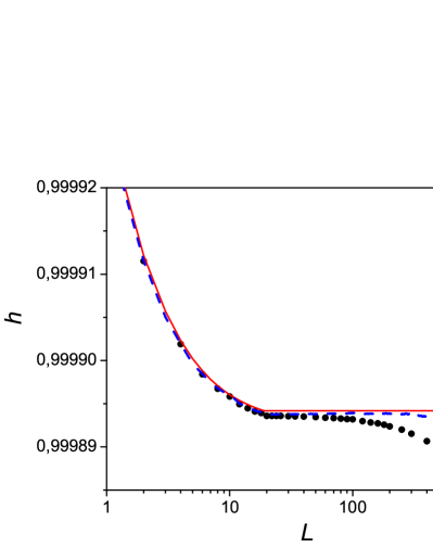
Figure 1: The differential entropy vs the length $L$. The solid line is the analytical result, Eq. (22), for correlation function $K(r)=0.01/r^{1.1}$, whereas the dots correspond to direct evaluation of the same Eq. (22) for the numerically constructed sequence (of the length $M=10^{8}$ and the cut-off parameter $R_{c}=20$) by means of conditional probability function (14) and the numerically evaluated correlation function $K(r)$ of the constructed sequence. The dashed line is the differential entropy with fluctuation correction described by Eq. (29).

As an illustration of result (22), in Fig. 1 we present the plot of the differential entropy versus the length $L$. Both numerical and analytical results (the dotted and solid curves) are presented for the power-law correlation function $K(r)=0.01/r^{1.1}$. The cut–off parameter $R_{c}$ of the power-law function for numerical generation of the sequence, coinciding with the memory length of the chain, is $20$. The good agreement between the curves at $L<R_{c}$ is the manifestation of adequateness of the additive Markov chain approach for studying the entropy properties of random chains.

IV Finite random sequences

The relative average number of unities $\bar{a}$, correlation functions and other statistical characteristics of random sequences are deterministic quantities in the limit of their infinite lengths only. It is a direct consequence of the law of large numbers. If the sequence length $M$ is finite, the set of numbers $a_{1}^{M}$ cannot be considered anymore as ergodic sequence. In order to restore its status we have to introduce the ensemble of finite sequences $\{a_{1}^{M}\}_{p},p\in\mathbb{N}=0,1,2,...$. Yet, we would like to retain the right to examine finite sequences by using a single finite chain. So, for a finite chain we have to replace definition (12) of the correlation function by the following one,

$$C_{M}(r) = \frac{1}{M-r}\sum_{i=0}^{M-r-1}(a_{i}-\bar{a})(a_{i+r}-\bar{a}),$$

$$\bar{a} = \frac{1}{M}\sum_{i=0}^{M-1}a_{i}.$$ (23)

Now the correlation functions and $\bar{a}$ are random quantities which depend on the particular realization of the sequence $a_{1}^{M}$. Their fluctuations can contribute to the entropy of finite random chains even if the correlations in the random sequence are absent. It is well known that the order of relative fluctuations of additive random quantity (as, e.g., the correlation function Eq. (IV)) is $1/\sqrt{M}$.

Below we give more rigorous justification of this explanation and show its applicability to our case. Let us present the correlation function $C_{M}(r)$ as the sum of two components,

$$C_{M}(r)=C(r)+C_{f}(r),$$ (24)

where the first summand $C(r)=\lim_{M\rightarrow\infty}C_{M}(r)$ is the correlation function determined by Eqs. (12) and (IV), obtained by averaging over the sequence with respect to index $i$, enumerating the elements $a_{i}$ of sequence $\mathbb{A}$; and the second one, $C_{f}(r)$, is a fluctuation–dependent contribution. Function $C(r)$ can be also presented as the ensemble average $C(r)=\langle C_{M}(r)\rangle$ due to the ergodicity of the sequence.

Now we can find a relationship between variances of $C_{M}(r)$ and $C_{f}(r)$. Taking into account Eq. (24) and the properties $\langle C_{f}(r)\rangle=0$ at $r\neq 0$ and $C(r)=\langle C_{M}(r)\rangle$ we have

$$\langle C^{2}_{M}(r)\rangle=C^{2}(r)+\langle C^{2}_{f}(r)\rangle.$$ (25)

The mean fluctuation of squared correlation function $C^{2}_{f}(r)$ is

$$\langle C^{2}_{f}(r)\rangle=$$ (26)

$$\!\!\!\frac{1}{(M-r)^{2}}\langle\!\!\!\sum_{n,m=0}^{M-r-1}\!\!\!(a_{n}-\bar{a})(a_{n+r}-\bar{a})(a_{m}-\bar{a})(a_{m+r}-\bar{a})\rangle.$$

Taking into account that only the terms with $n=m$ give nonzero contribution to the result and neglecting correlations between elements $a_{n}$,

$$\langle \sum_{n,m=0}^{M-r-1}(a_{n}-\bar{a})(a_{n+r}-\bar{a})(a_{m}-\bar{a})(a_{m+r}-\bar{a})\rangle$$

$$= \sum_{n=0}^{M-r-1}\langle(a_{n}-\bar{a})^{2}\rangle\langle(a_{n+r}-\bar{a})^{2}\rangle=(M-r)\,\,C^{2}_{f}(0).$$

we obtain for the normalized correlation function

$$\langle K^{2}_{f}(r)\rangle=\frac{\langle C^{2}_{f}(r)\rangle}{C^{2}_{f}(0)},\,\,\langle K^{2}_{f}(r)\rangle=\frac{1}{M-r}\simeq\frac{1}{M}.$$ (28)

Note that Eq. (28) is obtained by means of averaging over the ensemble of chains. This is the shortest way to obtain the desired result. At the same time, for numerical simulations we have used only the averaging over the chain as is seen from Eq. (IV), where the summation over sites $i$ of the chain plays the role of averaging.

Note also that the different symbols $a_{i}$ in Eq. (26) are correlated. It is possible to show that contribution of their correlations to $\langle K^{2}_{f}(r)\rangle$ is of order $R_{c}/M^{2}\ll 1/M$.

The fluctuating part of entropy, proportional to $\sum_{r=1}^{L}K^{2}_{f}(r)$, should be subtracted from Eq. (22), which is only valid for the infinite chain. Thus, Eqs. (25) and (28) yield the differential entropy of the finite binary weakly correlated random sequences

$$h_{L}=h_{0}-\frac{1}{2\ln 2}\left[\sum_{r=1}^{L}K_{M}^{2}(r)-\ln\frac{M}{M-L}\right].$$ (29)

It is clear that in the limit $M\rightarrow\infty$ this function transforms into Eq. (22). When $L\ll M$, the last term in rhs of Eq. (29) takes the form $L/M$ and describes the linearly decreasing entropy.

The squared correlation function $K^{2}_{M}(r)$ is normally a decreasing function of $r$, whereas function $K^{2}_{f}(r)$ is an increasing one. Hence, the terms $\sum_{r=1}^{L}K_{M}^{2}(r)$ and $\ln[M/(M-L]$ being concave and convex functions, respectively, describe the competitive contributions to the entropy. It is not possible to analyze all particular cases of their relationship. Therefore we indicate here the most interesting ones taking in mind monotonically decreasing correlation functions. An example of such type of function, $K(r)=a/r^{b},\,a>0,\,b\geq 1$, was considered above.

If the correlations are extremely small and compared with the inverse length $M$ of the sequence, $K_{M}^{2}(1)\sim 1/M$, the fluctuating part of the entropy exceeds the correlation part nearly for all values of $L>1$.

With the increasing of $M$ (or correlations), when the inequality $K_{M}^{2}(1)>1/M$ is fulfilled, there is at list one point where the contribution of fluctuation and correlation parts of the entropy are equal. For monotonically decreasing function $K(r)$ there is only one such point. Comparing the functions in square brackets in Eqs. (29) we find that they are equal at some $L=R_{s}$, which hereafter will be referred to as a stationarity length. If $L\ll R_{s}$, the fluctuations of the correlation function are negligibly small with respect to its magnitude, hence the finite sequence may be considered as quasi-stationary one. At $L\sim R_{s}$ the fluctuations are of the same order as the genuine correlation function $K^{2}(r)$. Here we have to take into account the fluctuation correction due to the finiteness of the random chain. At $L>R_{s}$ the fluctuating contribution exceeds the correlation one.

The other important parameter of the random sequence is the memory length $N$. If the length $N$ is less than $R_{s}$, we have no difficulties to calculate the entropy of the finite sequence, which can be considered as quasi-stationary. This case is illustrated in Fig. 1 where the good agreement between the analytical and numerical curves at $L<R_{c}$ is clearly seen. If the memory length exceeds the stationarity length, $R_{s}\lesssim N$, we have to take into account the fluctuation correction to the entropy. The entropy with this correction is shown in Fig. 1 by the dashed line. Two types of different relationships between memory length $N$ and stationarity length $R_{s}$ are shown in Fig. 2. Note that at $L>N$ the entropy does not change. Two solid points in the figure correspond to the equality $L=N$.

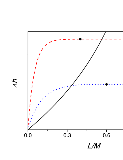
Figure 2: The dotted and dashed lines are $M$-independent contributions to the entropy, $\sum_{r=1}^{L}K_{M}^{2}(r)\,/\,2\ln 2$, see Eq. (29), for two different memory lengths marked by two solid dots. Both lines correspond to exponential correlator $K(r)\propto\exp(-r/r_{0})$. For the dashed line $r_{0}=0.1M$ and correlation length is $r_{c}=0.4M$. The dotted line represents a sequence with $r_{0}=0.2M$ and $r_{c}=0.6M$. The solid line is the fluctuation correction $\ln[M/(M-L)]\,/\,2\ln 2$.

V Entropy of DNA sequences

It is known that any DNA text is written by four “characters”, specifically by adenine (A), cytosine (C), guanine (G), and thymine (T). Therefore, there are three nonequivalent types of the DNA text mapping onto one-dimensional binary sequences of zeros and unities. The first of them is the so-called purine-pyrimidine rule, {A,G} $\rightarrow$ 0, {C,T} $\rightarrow$ 1. The second one is the hydrogen-bond rule, {A,T} $\rightarrow$ 0, {C,G} $\rightarrow$ 1. And, finally, the third is {A,C} $\rightarrow$ 0, {G,T} $\rightarrow$ 1.

Figure 3: The dependence $D(L)$ for the coarse-grained DNA text of Bacillus subtilis, complete genome  ftp , for three nonequivalent kinds of mapping. Dotted, dashed, and dash-dotted lines correspond to the purine-pyrimidine mapping, {A,G} $\rightarrow$ 0, {C,T} $\rightarrow$ 1; hydrogen-bond rule mapping, {A,T} $\rightarrow$ 0, {C,G} $\rightarrow$ 1; and {A,C} $\rightarrow$ 0, {G,T} $\rightarrow$ 1, respectively. The solid line describes the non-correlated Brownian diffusion, $D(L)=L/4$.

In order to understand which kind of mapping is more appropriate for calculating the entropy, we consider all three kinds of mapping UYa . As an example, the variance $D(L)=\overline{k^{2}}-\overline{k}^{2},k_{i}(L)=\sum\limits_{l=1}^{L}a_{i+l}$ for the coarse-grained text of Bacillus subtilis, complete genome ftp , is displayed in Fig. 3 for all possible types of mapping. The different kinds of mapping reveal and emphasize various types of physical attractive correlations between the nucleotides in the DNA, such as the strong purine-purine and pyrimidine-pyrimidine persistent correlations (the upper curve), and the correlations caused by the weaker attraction A$\leftrightarrow$T and C$\leftrightarrow$G (the middle curve). In what follows we will use the purine-pyrimidine coarse-grained mapping, which corresponds to the strongest correlations.

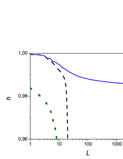
Figure 4: Differential entropy $h$ vs length $L$ for R3 chromosome of Drosophila melanogaster DNA of length $M\simeq 2.7\times 10^{7}$. The solid line is obtained by using Eq. (22) with numerically evaluated correlation function Eq. (12). The dashed line is the differential entropy, Eqs. (15) and (16), plotted by using the numerical estimation of probability $P(a_{1},\ldots,a_{L})$ of the $L$-blocks occurring in the same sequence. The dots are the differential entropy (normalized by division by 2) of the same sequence, Eqs. (15) and (16), without coarse-graining, i.e., for four-letter DNA sequence.

In order to evaluate the entropy of DNA sequence using Eq. (22) at first we have to calculate the normalized correlation function given by Eq. (12), where each random variable $a_{i}$ after mapping takes on the values $0$ or $1$. The result of such calculation for R3 chromosome of Drosophila melanogaster DNA of length $M\simeq 2.7\times 10^{7}$ is shown in Fig. 4 by the solid line. The abrupt deviation of the dashed line from the upper curves at $L\sim 10$ is the result of violation of inequality (2) and the manifestation of rapidly growing errors in the entropy estimation by using the probability $P(a_{1},\ldots,a_{L})$ of the $L$-blocks occurring. The dotted curve shows that the violation of strong inequality (2) for four-letter sequence begins at smaller value of $L$ than for two-letter (binary) sequence.

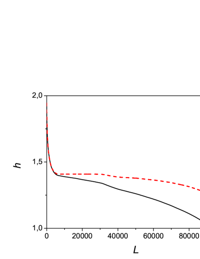
Figure 5: The differential entropy of Homo sapiens chromosome Y, locus NW 001842422 vs length $L$. The solid line is obtained by using the equation similar to Eq. (22) with numerically evaluated correlation functions. The dashed line is the entropy with the fluctuation correction.

The theory of additive Markov chains presented here can be applied to the chains with $d$-valued space of states. In our case $d=4$. Using the formula similar to Eq. (29) we evaluate the entropy for Homo sapiens chromosome Y, locus NW 001842422. The result of calculation is shown in Fig. 5. It is clearly seen that the entropy in interval $7\times 10^{3}<L<3\times 10^{4}$ takes on the constant value, $h_{L}\simeq 1.41$. It means that for $L>7\times 10^{3}$ all correlations, in the statistical sense, are taken into account, or, in other words, the memory length of the Homo sapiens chromosome Y is of the order of $10^{4}$. At $L>3\times 10^{4}$ the entropy evidently should be constant as well. The presented deviation is the consequence of many different reasons such as the nonadditivity of the sequence under study, the violation of supposed weakness of correlations, and many others.

We believe that, along with the memory length, the asymptotic value of the entropy $h_{L}$ at $L\rightarrow\infty$ (the Shannon source entropy) can be the important characteristics of the living species.

VI Conclusion and perspectives

1. This paper is the first application of the theory based on the additive Markov chains approach for describing the DNA sequences. It is evident that we need a more systematic and extensive study of the real biological sequences.

2. We have supposed that correlations are weak. However, our preliminary study evidences that when correlations are not weak, a strong short-range part in the interaction of symbols changes in Eq. (22) the numerical coefficient before the term $\sum_{r=1}^{L}K^{2}(r)$ at $L\rightarrow\infty$.

3. Our consideration can be generalized to the Markov chain with the infinite memory length $N$. In this case we have to impose a condition on the decreasing rate of the correlation function and the conditional probability function at $N\rightarrow\infty$. Another generalization, which may be important for biological applications  Raftery ; Cocho ; Tavare ; Borodovsky , is the non-homogenous Markov chains. In this case the conditional probability function $P$ has to be the function of the position $i$ of symbol $a_{i}$,

$$P=P(a_{i}=a|i,a_{i-N},\ldots,a_{i-2},a_{i-1}).$$ (30)

4. It would be interesting to compare the result obtained in our work with that of the Lempel-Zive approach Cover and the hidden Markov chain model Seifert .

5. In this paper we have considered the random sequences with the binary space of states, but almost all results can be generalized to non-binary sequences.

- (1) Buldyrev, S.V. et al, 1995. Long-range correlation properties of coding and noncoding DNA sequences: GenBank analysis. Phys. Rev. E. 51, 5084.
- (2) Almirantis, Y., Provata, A., 1999. Long- and Sort-Range Correlations in Genome Organisation. J. Stat. Phys., 97, 233.
- (3) Madigan, M.T., Martinko, J.M., Parker, J., 2002. Brock Biology of Microorganisms, Prentice Hall.
- (4) Ehrenfest, P., Ehrenfest, T, 1911. Encyklopädie der Mathematischen Wissenschaften, Berlin: Springer.
- (5) Lind, D., Marcus, B., 1995. An Introduction to Symbolic Dynamics and Coding, Cambridge University Press.
- (6) Shannon, C.E., Weaver, W., 1949. The Mathematical Theory of Communication, University of Illinois Press.
- (7) Cover, T.M., Thomas, J.A., 1991. Elements of Information Theory, Wiley, New York.
- (8) Melnyk, S.S., Usatenko O.V., Yampol’skii, V.A., 2006. Memory functions of the additive Markov chains: applications to complex dynamic systems. Physica A, 361, 405.
- (9) Usatenko O.V., Apostolov, S.S., Mayzelis Z.A., Melnik, S.S., 2010. Random finite-valued dynamical systems: additive Markov chain approach, Cambridge Scientific Publisher, Cambridge.
- (10) Raftery, A., 1985. A model for high-order Markov chains. Journal of Royal Statistical Society B, 47, 528-539.
- (11) Ching, W.K., Fung, E.S., Ng, M.K., 2004. Higher-order Markov chain models for categorical data sequence. Naval Research Logistics, 51, 557-574.
- (12) Li, W.K., Kwok, M.C.O., 1990. Some results on high order Markov chain models. Communications in Statistics - Simulation and Computation, 19, 363-380.
- (13) Cocho, J.A. et al, Bacterial genomes lacking long-range correlations may not be modeled by low-order Markov chains, this issue.
- (14) Seifert, M., Gohr, A., Strickert, M., Grosse, I., 2012. Parsimonious higher-order hidden Markov models for improved array-CGH analysis with applications to Arabidopsis thaliana, PLoS Computational Biology, 8, e1002286.
- (15) Shiryaev, A.N., 1996. Probability, Springer, New York.
- (16) Berchtold, A., 1995. Autoregressive modelling of Markov chains, in: Statistical Modelling, Lecture Notes in Statistics, vol 104, Springer, pp.19-26.
- (17) Chakravarthy, N., Spanias, A., Iasemidis, L.D., Tsakalis, K., 2004. Autoregressive modeling and feature analysis of DNA sequences, EURASIP J Applied Signal Processing, 1, 13-28.
- (18) Melnyk, S.S., Usatenko, O.V., Yampol’skii, V.A., Golick, V.A., 2005. Competition between two kinds of correlations in literary texts, Phys. Rev. E, 72, 026140.
- (19) Denisov, S.V., Melnik, S.S., Borisenko, A.A., Usatenko, O.V., Yampolsky, V.A., Entropy of complex symbolic sequences: Exact results; to be published.
- (20) Usatenko, O.V., Yampol’skii, V.A., 2003. Binary N -Step Markov Chains and Long-Range Correlated Systems, Phys. Rev. Lett., 90, 110601.
- (21) Raftery, A., Tavare, S., 1994. Estimation and modelling repeated patterns in high order Markov chains with the mixture transition distribution model, Applied Statistics, 43, 179-199.
- (22) Borodovsky, M., Peresetsky, A., 1994. Deriving Non-homogeneous Markov Chain Models by Cluster Analysis Algorithm Minimizing Multiple Alignment Entropy, Computers and Chemistry, 18, 259-268.
- (23) ftp:ftp.ncbi.nih.govgenomesbacteriabacillus_subtilis NC_000964.gbk.