The YSO Population in the Vela-D Molecular Cloud.

Abstract

We investigate the young stellar population in the Vela Molecular Ridge, Cloud-D (VMR-D), a star forming (SF) region observed by both Spitzer/NASA and Herschel/ESA space telescope. The point source, band-merged, Spitzer-IRAC catalog complemented with MIPS photometry previously obtained is used to search for candidate young stellar objects (YSO), also including sources detected in less than four IRAC bands. Bona fide YSO are selected by using appropriate color-color and color-magnitude criteria aimed to exclude both Galatic and extragalactic contaminants. The derived star formation rate and efficiency are compared with the same quantities characterizing other SF clouds. Additional photometric data, spanning from the near-IR to the submillimeter, are used to evaluate both bolometric luminosity and temperature for 33 YSOs located in a region of the cloud observed by both Spitzer and Herschel. The luminosity-temperature diagram suggests that some of these sources are representative of Class 0 objects with bolometric temperatures below 70 K and luminosities of the order of the solar luminosity. Far IR observations from the Herschel/Hi-GAL key project for a survey of the Galactic plane are also used to obtain a band-merged photometric catalog of Herschel sources aimed to independently search for protostars. We find 122 Herschel cores located on the molecular cloud, 30 of which are protostellar and 92 starless. The global protostellar luminosity function is obtained by merging the Spitzer and Herschel protostars. Considering that 10 protostars are found in both Spitzer and Herschel list it follows that in the investigated region we find 53 protostars and that the Spitzer selected protostars account for approximately two-thirds of the total.

1 Introduction

The Vela Molecular Ridge Cloud-D (hereafter VMR-D) ($260\arcdeg\lesssim\ell\lesssim 264\arcdeg$; $\left|b\right|\lesssim 1\arcdeg$) is part of a giant molecular complex located along the Galactic plane ($260\arcdeg\lesssim\ell\lesssim 272\arcdeg$; $\left|b\right|\lesssim 3\arcdeg$ Murphy & May, 1991) and is then well suited to represent a typical star forming region (SFR) of our Galaxy. For this reason a subregion of this cloud has been the subject of many previous papers, dealing with different observational aspects of the star formation (SF) as, e.g., the presence of outflows (Wouterloot & Brand, 1999; Elia et al., 2007), jets (Lorenzetti et al., 2002; Giannini et al., 2005, 2013), and clustering (Massi et al., 2000). The continuum submillimeter emission in the VMR-D cloud was surveyed by Massi et al. (2007) who catalogued 29 resolved dust cores and also obtained a further list of 26 unresolved candidate cores. More recently, thanks to the opportunity offered by the Spitzer Space Telescope, the VMR-D region was observed with the IRAC ($\lambda$ = 3.6, 4.5, 5.8, 8.0 $\mu$m) and MIPS ($\lambda$ = 24, 70 $\mu$m) focal plane instruments, obtaining in this way six mosaics, covering about 1.2 deg², that have been analyzed to produce a merged photometric Spitzer-IRAC point-source catalog (hereinafter Spitzer-PSC) complemented with MIPS photometry (Strafella et al., 2010, hereinafter Paper I). Further observational progress was made when the BLAST experiment (Pascale et al., 2008) mapped the whole Vela Molecular Ridge in the far-IR (FIR) spectral region ($\lambda$ = 250, 350, 500 $\mu$m), complementing in this way the Spitzer spectral coverage towards long wavelengths. These observations were discussed by Olmi et al. (2009) who obtained a catalog of dense cores/clumps in the VMR-D cloud. The last important observational progress was made with the Herschel Space Observatory which, surveying the Galactic plane in the framework of the Hi-GAL key project, partially mapped the VMR-D region in the FIR spectral range ($\lambda$ = 70, 160, 250, 350, 500 $\mu$m) with an almost double spatial resolution and sensitivity with respect to BLAST. Here we also analyze these observations for the first time, thanks to the support of the Hi-GAL collaboration that provided us with the corresponding calibrated maps. These have been used to extract five single band photometries that constitute another important spectral extension of our information about this region.

Utilizing these observations as well as the photometric catalogs made available by the 2MASS and WISE all-sky surveys, we have the opportunity to study in much more detail the young stellar objects (YSOs) located in the VMR-D cloud. These objects can be efficiently identified through their infrared colors (see, e.g., Harvey et al., 2007; Gutermuth et al., 2009; Kryukova et al., 2012) that we also exploit here to discriminate genuine YSOs from other contaminant populations of both Galactic and extragalactic origin. All these observational data and tools give us the opportunity to investigate, with unprecedented sensitivity and accuracy, the characteristics of the SF in the VMR-D cloud.

In Paper I, we already considered a subsample of 8796 sources, detected in all the four IRAC bands out of the $\approx$ 170,000 sources listed in the Spitzer-PSC, to carry out a preliminary study of the YSO population in this cloud. Here, to obtain a more complete and accurate view, we revisit our previous preliminary census of the YSOs by including, besides the sources already considered in Paper I, all the other sources detected in at least two out of the four IRAC bands, with the additional requirement that sources detected in only two bands are also detected in the MIPS 24 $\mu$m band.

As in Paper I, we adopt the usual classification of the YSOs based on the near and mid-IR spectral slope defined as $\alpha=d(\log{\lambda F_{\lambda}})/d(\log{\lambda})$, a parameter originally introduced by Lada (1987) to characterize the spectral energy distribution (hereinafter SED) of these objects that is still largely used and generally interpreted as a proxy of the evolutionary phases experienced by the YSOs. In this scheme, it is customary to distinguish four different classes of YSOs, according to the value of this slope in 2 $\lesssim\lambda(\mu$m)$\lesssim$ 20 spectral interval : Class I with $\alpha>0.3$, flat spectrum (hereinafter FS) for $-0.3<\alpha<0.3$, Class II for $-1.6<\alpha<-0.3$, and finally Class III showing $\alpha<-1.6$. Given the evolutionary significance usually attributed to this parameter (but see also Chen et al., 1995; Young & Evans, 2005, for alternative schemes), Class I objects represent an early phase in the evolutionary path of the YSOs towards the ZAMS. Their spectral slope is produced by a central object that already attained its entire initial main-sequence mass, but is still surrounded by a remnant infall envelope and possibly an accretion disk. This description naturally implies the existence of an even earlier phase, the Class 0 as originally suggested by André et al. (1993), in which the central object is at the end of the free-fall phase but is still increasing its mass by accreting material from a thick surrounding envelope. This fact makes the Class 0 phase difficult to detect in the near IR and then difficult to classify in the framework of the aforementioned scheme. In this observational classification both Class 0 and I are representative of early protostars still surrounded by a remnant infall envelope, although only in the Class 0 stage the envelope is presumed to be more massive than the central object and then opaque to near and possibly also to mid-IR wavelengths (both ranges hereinafter referred to as MIR).

To study the SF mechanism in the VMR-D cloud we proceed along two approaches, both aimed to select candidate protostellar sources by exploiting all the information collected on the continuum emission. The first consists in selecting protostellar candidates by analyzing the Spitzer observations through a pipeline based on the criteria used by Harvey et al. (2007) and Gutermuth et al. (2009), that have been proven to be effective in isolating different kinds of possible contaminant sources. In the following, we shall refer to these sources as “Spitzer selected” and their analysis will be based on the SEDs assembled by collecting all the available photometries in what we shall call the MIR catalog. The second approach adopts the FIR point of view because it is based on the analysis of the Herschel observations that, being carried out at longer wavelengths, are more sensitive to cold and young protostars. The sources selected in this way will be referred to as “Herschel selected” and their SEDs will be arranged in the FIR catalog resulting from the Herschel photometry complemented with all the available photometries at shorter and longer wavelengths. Merging the results obtained in these two ways we expect to obtain a more complete view of the protostellar population in VMR-D as well as new insights on the SF process in this molecular cloud.

In the following, a brief account of the observational data obtained with Spitzer and Herschel is given in Section 2 along with a description of the procedures involved in data reduction and photometry. This section also illustrates how we obtain two multiwavelength source catalogs for the VMR-D region. The first, called MIR catalog, by complementing our previous Spitzer-PSC catalog with a set of additional observational data and the second, the FIR catalog, by assembling the five band Herschel photometry in a single band-merged list of sources.

In Section 3 we select bona fide YSOs out of both catalogs by means of appropriate selection criteria and in Section 4 we discuss the census and classification of these sources. We also obtain a new estimate of the SF rate and efficiency that is more accurate than that obtained in Paper I based on the sole sources detected in all the four IRAC bands.

In Section 5, bolometric temperatures and luminosities are derived for all those sources for which a reasonably complete photometric information is available. Here the L_bol vs T_bol diagram is used to further characterize the YSOs and infer on their evolutionary status.

In Section 6 we compare the SF rate and efficiency obtained for VMR-D with those obtained in other SFRs and discuss the global protostellar luminosity function (PLF). For those sources detected by Herschel at FIR wavelengths, the envelope mass has been also derived by exploiting a simple modified blackbody model. The luminosity-mass diagram is briefly discussed in the light of the protostellar evolutionary scenario.

Finally, in Section 7, our conclusions are summarized.

2 Observational Data

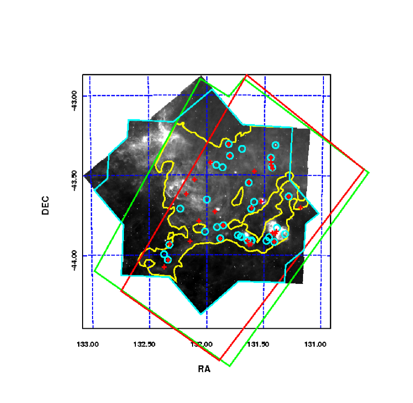
Figure 1: IRAC 8.0 $\mu$m image of the VMR-D investigated field with the positions of the Spitzer (cyan circles) and Herschel (red crosses) protostellar sources located ON-cloud and in the common area surveyed by both Spitzer and Herschel. The cyan polygon delimit the coverage of the Spitzer-PSC catalog (Paper I), while the large tilted trapezoids delimit the coverage of the Herschel SPIRE (green) and PACS (red) Hi-GAL observations analyzed in this work. The yellow contour line corresponds to a column density N(H${}_{2})=6.5\times 10^{21}$ cm^-2 and delimits the region we consider ON-cloud (see text). For a normal interstellar extinction curve this corresponds to $A_{V}\sim 3.5$ mag.

The observational data on the continuum emission of the objects in VMR-D have been collected from many different sources including existing catalogs, public surveys, and new observations as in the case of the Herschel unpublished photometry. Dealing with a conspicuous amount of observational material spread over quite a large spectral interval, we decided to search for candidate YSOs exploiting all the spectral characteristics of their continuum emission. Our approach is twofold and corresponds to adopt a “MIR point of view” as well as a “FIR point of view” to identify protostellar candidates by means of procedures typically adopted in previous studies of SFRs observed with Spitzer and Herschel, respectively. In the following, to identify the sky regions involved in the different observations of the VMR-D cloud, we shall refer to Figure 1 that shows the 8 $\mu$m IRAC image of the VMR-D cloud with overlayed the contours delimiting the areas observed by different instuments as well as the contour of the investigated cloud.

2.1 MIR catalog

We start considering the sources of the Spitzer-PSC catalog covering the region delimited by the cyan polygon in Figure 1. To arrange all of the available continuum observations for an easy access and at the same time obtain the SEDs, we generated a new catalog containing the fluxes from all the available photometric surveys of this cloud from the near-IR to the submillimeter spectral range. This catalog is essentially a spectral extension of our previous Spitzer-PSC catalog and contains, besides the Spitzer-IRAC/MIPS (3.6, 4.5, 5.8, 8.0, 24, 70 $\mu$m) photometry, also 2MASS (J, H, K bands), WISE (3.4, 4.6, 12, and 22 $\mu$m), Herschel (70, 160, 250, 350, and 500 $\mu$m), and SEST-SIMBA (1200 $\mu$m) observations.

Given the heterogeneous nature of the observational data, we adopted specific criteria in associating to the same source fluxes obtained at different wavelengths and with different spatial resolutions. This is a typical problem in assembling information coming from different catalogs and it is usually mitigated by requiring that the distance between the centroids of the sources to be associated is smaller than a predetermined value depending on the spatial resolution of the specific catalogs. This is also our approach even if more complex association procedures could be devised, involving further considerations on the flux values to be associated and, in turn, on the possible underlying spectral shapes (see, e.g., Roseboom et al., 2009; Budavari & Szalay, 2008). In our case we prefer to consider the positional uncertainty, instead of the beamsize, as a measure of the spatial accuracy of a given catalog because it is usually evaluated after an accurate statistical analysis and is generally more conservative. In this way we minimize possible mismatches in associating to the same source the fluxes from different catalogs, especially in crowded regions, even if we pay this choice with the risk to miss some source association.

Our procedure adopts the fiducial positions of the sources reported in the Spitzer-PSC catalog, in this way considering the other catalogs as ancillary, and are used to find possible counterparts at other wavelengths. The final product is a catalog containing the same number of entries as the Spitzer-PSC, but complemented with the associated fluxes observed at different wavelengths. In Table 1 we report the association radii adopted for the catalogs considered in this work, along with the associated beamsizes, completeness fluxes, and relevant references.

In practice, we consider as acceptable the associations for which the distance $\Delta\theta$ between the position of the Spitzer-PSC source and the position of a source in a given catalog is less than the sum of the corresponding uncertainties, namely $\Delta\theta~{}<~{}\delta\theta_{\mathrm{PSC}}+\delta\theta_{\mathrm{cat}}$. In the case of multiple associations we always adopt the nearest source to the fiducial Spitzer-PSC position, allowing however that multiple Spitzer-PSC sources could be similarly associated to the same object of another catalog, a problem that will be taken into account later in the analysis. After scanning all the considered catalogs for positional association with the Spitzer-PSC sources we obtained a set of corresponding fluxes that, once assembled, constitute the MIR multiwavelength catalog of our interest.

2.2 FIR catalog

The VMR-D cloud is located across the Galactic plane and it has been partially mapped by the Herschel space telescope during the completion of the Hi-GAL key project for a FIR survey of the Galactic plane (Molinari et al., 2010). As is shown in Figure 1 the survey coverage is incomplete because at these longitudes the observing strategy of the Hi-GAL survey preferred to follow the warp of the Galaxy instead of the Galactic plane. The VMR-D cloud has been also mapped by the BLAST experiment at 250, 350 and 500 $\mu$m albeit with a significantly lower spatial resolution and sensitivity. Because of this, in the following we prefer to use the Herschel observations instead of the BLAST ones, alleviating in this way the problems related to both the strong and variable background and the source confusion.

Thanks to the Hi-GAL consortium we obtained calibrated maps (Bernard et al., 2000) of our region in which the artifacts introduced by the map-making technique have been removed or heavily attenuated by means of a weighted post-processing of the maps themselves (Piazzo et al., 2012). The source detection and photometry has been carried out on these maps by using the CuTeX package (Molinari et al., 2011), a software specifically designed to detect and extract compact sources against a strong and variable background. In this way we obtained five lists of sources, corresponding to the five bands of the Hi-GAL survey, that have been merged adopting the association radii reported in Table 1 for the Herschel photometry. In assembling this catalog the merging process proceeded from long to short wavelengths, updating the position of each merged source with the coordinates corresponding to the source actually associated at the shortest wavelength, with the aim to retain the position associated to the shortest detected wavelength.

Subsequently, to evaluate accurate bolometric quantities, we also extended the spectral information on these FIR sources by complementing the merged Herschel catalog with Spitzer and WISE fluxes, at shorter, and with 1.2 mm SIMBA fluxes (Massi et al., 2007), at longer wavelengths. In doing this we always adopt the positional requirements reported in Table 1 to associate complementary fluxes to the fiducial positions in the multiband catalog of the Herschel sources.

As for the previous MIR catalog, the merging procedure allows the possibility of multiple source associations, within the constraints in Table 1), a problem that will be taken into account in the subsequent analysis of this FIR catalog.

3 Sources Selection

To obtain a census as complete as possible of the protostellar content in the VMR-D cloud we exploit both the MIR and FIR catalogs based on the Spitzer and Herschel observations, respectively. Because in the following analysis we select candidate protostars from these catalogs, here we separately illustrate the selection procedure and the classification criteria adopted to characterize the selected sources.

3.1 MIR sources

A preliminary analysis, limited to the Spitzer sources detected in all the four IRAC bands, was already presented in Paper I. Here we enlarge the data base to all the sources detected with photometric uncertainties $\sigma<0.2$ mag in at least three out of the four IRAC bands, augmented with those sources that, detected only in two IRAC bands, are also detected in the MIPS 24 $\mu$m band. As a final addition, with the aim to consider potentially interesting objects, we also include a few special cases that, detected in only one IRAC band, are particularly bright at $\lambda=24~{}\mu$m and show a spectral slope that is compatible with a Class I SED.

While including sources detected in only three wavelengths helps mitigate possible selection effects due to different sensitivities in the IRAC bands, considering also objects detected in only two IRAC bands and in the MIPS 24 $\mu$m band allows us to include further sources that, for different reasons, could appear faint in particular wavelengths as, e.g., transition disks with large inner holes or unusual circumstellar geometries that could escape detection in some IRAC bands. The last addition of sources detected only in one IRAC band aims to include potentially interesting sources that could represent deeply embedded objects barely visible in the IRAC bands or even Class II sources with inner disk cleared from dust.

In this way we extracted a total number of 16391 sources whose distribution in the different typologies is shown in the first row of Table 2. These constitute the working data base in which we search for candidate YSOs by using specific selection criteria aimed to exclude both Galactic and extragalactic contaminants.

3.1.1 Selection phase

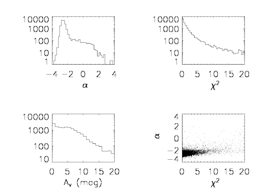
Figure 2: Best fit parameters obtained after comparing the observed MIR SEDs with the reddened photospheric emission models (see text). Upper panels: distribution of the spectral slopes $\alpha$ (left) and the reduced $\chi^{2}$ values (right) obtained by fitting the SEDs. Lower panels: the distribution of the visual extinctions A_V corresponding to the best-fits (left) and the $\alpha$ vs $\chi^{2}$ scatter plot (right).

The first obvious step in selecting bona fide YSOs is to exclude from further investigation all those sources that could be interpreted as reddened stellar photospheres. To this aim, following Harvey et al. (2006), we compared the observed with the model fluxes, based on the stellar photosphere Kurucz-Lejeune models, taken from the SSC’s Star-Pet tool . These fluxes are given just as they would be observed in the IRAC and MIPS bands and are then directly comparable with our observational data. In this respect, we scrutinized all the sources with at least three detections in the $2.2\leq\lambda\leq 24~{}\mu$m spectral region and, considering the effects of the extinction law given by Flaherty et al. (2007), we found 12217 sources that can be reasonably fitted with a reduced $\chi^{2}<2.5$ and then represent, most probably, reddened photospheres that have been consequently excluded from further consideration. With this choice the probability that some reddened normal star still contaminates our sample despite this filtering is less than $\sim 10\%$, a risk that will be further mitigated by the subsequent selection steps. In Figure 2 we show the distribution of the parameters involved in this procedure, noting that the bulk of the sources excluded by the adopted cut in $\chi^{2}$ involves essentially objects with slopes $-3.5~{}\lesssim~{}\alpha~{}\lesssim-1.5$ (bottom right panel) .

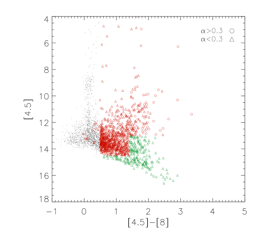
Figure 3: The IRAC color-magnitude diagram [4.5] vs [4.5]-[5.8] showing the position of different objects. Points represent background stars, triangles and circles are objects with $\alpha<0.3$ and $\alpha>0.3$, respectively. Green and red symbols indicate objects that are rejected and passed, respectively, after applying the Harvey et al. (2007) criteria (see text).

After this preliminary step (Step 1 in Table 2) we are left with 4174 sources that have been further filtered adopting the selection criteria used by Harvey et al. (2007, see their Tab.1) to identify extragalactic contaminants on the basis of the 4.5, 8.0, and 24 $\mu$m photometry. In this phase we also discarded sources with both color [4.5]-[8.0] $<$ 0.7 and spectral slope $\alpha~{}<-1.6$ as representing normal background stars remaining even after the previous dereddening phase and visible in Figure 3 as a cloud of small black points. Applying these criteria to our sample we eliminate 2217 sources whose different typologies are reported in the row labeled “Step 2” in Table 2.

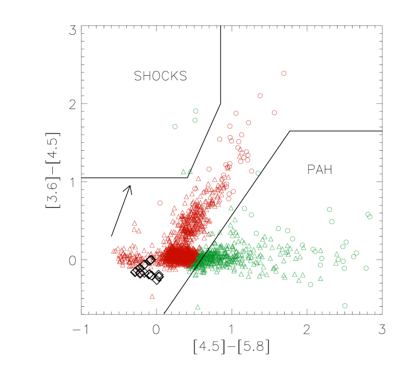
Figure 4: Color-color diagram exploiting IRAC fluxes to select candidate YSOs according to the Gutermuth et al. (2009) criteria. The reddening vector is also shown, corresponding to a visual extinction A_V=50 mag and to the reddening law determined by Flaherty et al. (2007). Symbols are as in Fig.3, except the black diamonds, in the lower left corner, that represent the locus of the stellar photospheres.

Excluding also these objects we count 1957 sources that have been further scrutinized with additional color-color and color-magnitude criteria similar to those devised by Gutermuth et al. (2009, their appendix A) to identify, and then exclude, further extragalactic as well as Galactic contaminants. Following these authors our sources have been examined in three different phases, the first consisting in the identification of sources whose colors are compatible with PAH contamined galactic and extragalactic sources, AGN, and protostellar shocks. In this phase 484 sources (Step 3 row in Tab. 2) were flagged as contaminants so that, excluding them from further consideration, we remain with 1473 sources. In Figure 4 the [3.6]-[4.5] vs [4.5]-[5.8] diagram is shown with the two regions, delimited by the continuous line, corresponding to the colors appropriate for shocks (upper left) and PAH contamined (lower right) sources (see also Gutermuth et al., 2009, fig.15).

As in the second phase of Gutermuth et al. (2009, appendix A), to include possible YSOs detected only in the [3.6] and [4.5] bands but not at 24 $\mu$m, we reconsidered the whole catalog to select all the cases with fluxes in JHK[3.6][4.5] bands, but requiring a photometric uncertainty $\sigma<0.1$ mag in the JHK bands to minimize chances to pick-up sources only because of the additional uncertainty implied by the dereddening procedure at these shorter wavelengths. In this way we selected 48 sources that, however, do not satisfy the phase 2 criteria of Gutermuth et al. (2009, appendix A) and then leave unaffected the total number of candidate YSOs.

In the third phase we recovered sources that, although detected in only one IRAC band, are however bright at 24 $\mu$m. These are potentially interesting sources because they could represent deeply embedded objects barely visible in the IRAC bands or even Class II sources with inner disk cleared from dust. Because of this we include in our sample of candidate YSOs all the sources with bright MIPS 24 $\mu$m photometry ([24] $<$ 7) to mitigate extragalactic contamination, and color [X] - [24] greater than the corresponding color expected for a SED with slope $\alpha=-0.3$, namely [X] - [24] $>$ 5.43, 4.77, 4.10, 3.22 for the four bands, where [X] is the only available IRAC band photometry. In this way we recovered 4, 4, 0, and 1 sources with good photometry in the IRAC 3.6, 4.5, 5.8, and 8.0 $\mu$m bands, respectively, increasing to 1482 the total number of candidate YSOs. All of these nine additional sources also show good MIPS 24 $\mu$m photometry with $\sigma<0.2$ mag. Finally, we complete the selection by excluding 12 sources showing a particularly irregular SED that cannot be represented by a single slope (see Table 2 and section 4.1 ), suggesting they are the result of source confusion. The final list of candidate YSOs selected out of the Spitzer-PSC catalog is then constituted by 1470 sources.

3.2 FIR sources

Another starting point to select candidate protostellar sources in the VMR-D cloud can be adopted by using the Herschel observations that, arranged in a FIR catalog of compact sources as described in Section 2.2, can be exploited to analyze the SEDs. In this respect our approach to select candidate protostars is quite different because at FIR wavelengths the observations are more sensitive to colder objects, complementing in this way our view of the starforming process.

Basically, candidate sources are selected by adopting specific prescriptions (see also Giannini et al., 2012) aimed to exclude cases that, also due to confusion problems, appear as spectrally inconsistent. To this aim we first eliminate from our FIR-catalog the ambiguities due to the presence of multiple associations, retaining only the nearest one to the fiducial catalog position, namely that determined in the band merging phase (see section 2.2). Then, to prepare the analysis of the SEDs, we select the sources detected in at least three out of the four Herschel bands at $\lambda\geq 160~{}\mu$m, not peaking at 500 $\mu$m, and without a dip between three adjacent wavelengths. In addition, we also require that these sources appear as resolved at $\lambda_{\mathrm{ref}}=250~{}\mu$m, a reference wavelength we assume to correspond to an optically thin regime (Elia et al., 2013). All of these prescriptions are in view of exploiting a simple modified blackbody model to fit the Herschel FIR fluxes in the subsequent classification phase.

The SEDs selected in this way have been in fact fitted with a simple modified blackbody model that assumes an optically thin regime for wavelengths $\lambda>\lambda_{0}$ and an optical depth described by $\tau=(\nu/\nu_{0})^{\beta}$, where $\beta=2$ is appropriate for simple dust models and $\nu_{0}=c/\lambda_{0}$ is the frequency corresponding to $\tau=1$. The model fluxes are computed from the relation:

$$F_{\nu}=(1-\mathrm{e}^{-\tau_{\nu}})~{}B_{\nu}(T_{d})~{}\Omega$$ (1)

where $T_{d}$ is the dust temperature and $\Omega$ is the solid angle subtended by the source to the observer. The fact $\Omega$ can be observationally constrained clarifies our previous requirement for resolved sources so that, to this aim, we consider as spatially resolved all the sources with a deconvolved size satisfying:

$$\mathrm{FWHM}_{\lambda,\mathrm{dec}}=\sqrt{\mathrm{FWHM}_{\lambda}^{2}-\mathrm{HPBW}_{\lambda}^{2}}~{}>~{}0.6\times\mathrm{HPBW}_{\lambda}$$ (2)

where FWHM_λ is the observed source size and HPBW_λ is the instrumental half power beam width at the given wavelength. Whith these choices, and assuming the VMR-D distance of 700 pc (Liseau et al., 1992), the beam size and the minimum resolved size corresponds to $\sim$0.06 pc and $\sim$0.02 pc, respectively.

However, constraining $\Omega$ with the deconvolved size at $\lambda_{\mathrm{ref}}=250~{}\mu$m is not strictly appropriate at all wavelengths, due to the increase of the apparent size when colder and larger volumes becomes “visible” at longer wavelengths. For this reason, before applying the fitting procedure, we normalized the fluxes obtained at longer wavelengths to the same angular size by scaling them with respect to the ratio of the deconvolved sizes, namely FWHM${}_{\lambda_{\mathrm{ref}},\mathrm{dec}}$/FWHM_λ,dec. This treatment is justified by the expectation that the radial density law in the cores is of the kind $\rho(r)\propto r^{-2}$ implying for the mass that M(r)$\propto r$ (Shu, 1977), a situation that in absence of a strong temperature gradient suggests the aforementioned flux scaling at optically thin wavelengths (Motte & André, 2001; Giannini et al., 2012).

Finally, by using a fitting procedure based on the Levenberg-Marquardt technique (Markwardt, 2009) we derive best fitting values for T_d, and $\lambda_{0}$, in this way also checking that the best fits always occur for $\lambda_{0}<100~{}\mu$m, a posteriori justifying our assumption of an optically thin regime at $\lambda=250\mu$m.

4 Classification

Here we exploit the fluxes collected both in the MIR and in the FIR catalogs to classify the protostars and characterize the SF process in the VMR-D cloud. In the following we discuss two different schemes we use for classifying Spitzer and Herschel selected sources, respectively.

4.1 MIR sources

As described in the introduction, here we adopt the YSOs classification scheme based on the spectral slope as evaluated in the MIR spectral range, with the addition of a further class, the Class 0. The latter has been introduced to include objects in the earliest phases that are very faint or even undetected in the MIR, being more easily detected in the FIR/submillimetric range. The physical basis for this scheme relies on the evolutionary scenario in which a central object is initially surrounded by an envelope of gas and dust whose spectral importance decreases with time in favour of an emerging hotter circumstellar disk. The global spectral appearance consequently changes so that an external observer would classify the YSO depending on the MIR spectral slope and then on the elapsed time from the end of the envelope dominated phase corresponding to the Class 0 stage. However, due to the intrinsic MIR faintness during the Class 0 stage, the least evolved protostars cannot be efficiently identified in this spectral region so that other complementary classification schemes have been proposed that are based on different observables as, e.g., the bolometric luminosity and temperature (see Chen et al., 1995; Young & Evans, 2005), quantities we shall consider later.

Here we limit ourselves to classify the candidate YSOs by considering the spectral slope in the interval $2\lesssim\lambda(\mu\mathrm{m})\lesssim 24$ and to this aim we use all the available fluxes collected in the MIR catalog. Two distibutions are shown in Figure 5, corresponding to the slopes obtained for the YSOs located ON and OFF-cloud, 869 and 356 cases respectively. Hereinafter with ON-cloud sources we mean those projected within the yellow contour line shown in Figure 1, corresponding to N(H₂)=6.5$\times 10^{21}$ cm^-2 in the column density map obtained by exploiting the Herschel/Hi-GAL observations with the same procedure adopted by Elia et al. (2013). After regridding the 160, 250 and 350 $\mu$m maps onto the pixels of the 500 $\mu$m map, we computed the corresponding cold dust temperature and column density maps. This has been done by fitting the modified black body model in Equation (1) to the intensities observed at the different wavelengths in each pixel of our maps, assuming the optically thin case as a justified approximation at these wavelengths. Note however that in the region outside the Herchel-PACS coverage only the three SPIRE fluxes are available and then here we derive less accurate column density values.

The final contour line obtained, beyond delimiting the cloud that is visible on our maps, corresponds to a visual extinction of A${}_{V}\sim 3.5$ that is approximately the extinction beyond which the largest number of protostars are found in the Orion A molecular cloud (Lada et al., 2013) and the column density distribution in the Auriga I cloud enters the low density region of the cloud itself (Froebrich & Rowles, 2010).

Conversely the OFF-cloud sources, that we consider as representative of the background, are those located outside the previous contour line. Our cloud is embedded in a larger complex so that what we define background here could not represents the true Galactic background, but instead should be considered a mixture of two components, one associated to the same Vela cloud and the other to the field. Despite this ambiguity the subtraction of the OFF from the ON-cloud component, weighting for the corresponding solid angles, remains appropriate to estimate the consistency of the “genuine” ON-cloud population.

The two histograms in Figure 5 show that earlier classes are relatively more abundant in the ON-cloud region and simply reflect the statistics, obtained for the different classes at the end of the source classification phase, that is reported in Table 3. In this respect it is worth noting that the counts in Table 3 do not change significantly by moving the boundary line of the ON-cloud region up to $\sim$15% in column density.

In this analysis we also discarded 12 sources, reported in Table 2 as the Step 4 of the selection pipeline, because their SED is probably affected by confusion problems. For these sources the linear fit in the $\log({\lambda F_{\lambda}})$ vs $\log({\lambda})$ diagram could not reasonably account for their peculiar SED that appears monotonically decreasing up to 8 $\mu$m, reminiscent of a Class III, and then suddenly rising in the 24 $\mu$m band.

We note however that, despite our efforts in eliminating the background contamination, the number of Class III sources remains the most uncertain because the colors of the normal stars closely mimic those of this class. Consequently, the number of the Class III sources should be considered more as an upper limit than as an intrinsic characteristic of the cloud.

4.2 FIR sources

Our FIR catalog is based on the Herschel sources and thus it is expected to be particularly rich in cold objects. In principle such objects can be either early protostars or quiescent cores and then it is essential to devise some criterium to distinguish protostellar from starless cores. This task can be accomplished by considering that while starless cores should be characterized by a single cloud temperature, the protostellar ones are instead expected to show a temperature gradient just because they harbour a protostar. To this aim we use the modified blackbody model described by Equation (1) to fit the FIR spectral points, but excluding the 70 $\mu$m fluxes since at this short wavelength the emission more likely results from warmer material and is then useful to trace the early protostellar phases. In other words the observed 70 $\mu$m flux is taken as discriminating the protostellar/starless nature of the sources depending on its compatibility with the flux expected from the model that best-fits the SED at the longer wavelengts. Consequently, objects showing a 70 $\mu$m flux exceeding the model flux by more than 3$\sigma$ are considered protostars while in all the other cases, including those without a 70 $\mu$m detection, we simply classify the sources as starless. In this phase, to allow a reasonable fit of the SED at $\lambda>70~{}\mu$m, we only consider Herschel sources showing at least three detections in the $160\leq\lambda\leq 500~{}\mu$m spectral range.

This classification procedure is illustrated in Figure 6 where two typical fits obtained with the model in Equation (1) are shown. In both cases we obtain a reasonable fit at $\lambda>160~{}\mu$m but in the right panel the 70 $\mu$m flux is clearly in excess with respect to that expected on the basis of the model. Interpreting this as a signature for the presence of a hotter embedded source, we classify this object as a candidate protostar. The converse is valid for the left panel showing a source we classify as starless.

In this way we identified 31 protostellar and 100 starless sources in the overlap region covered by both Herschel and Spitzer observations (see Figure 1) that reduce to 30 and 92 objects, respectively, when we consider only those located in the ON-cloud region. Their positions are shown in Figure 1 as red crosses, superimposed to the Spitzer 8 $\mu$m map of the VMR-D region, and their distribution in sizes is shown in the left panel of Figure 7. The latter values are derived by using the deconvolved angular sizes observed at 250 $\mu$m and assuming a distance of 700 pc. Note that, because we need to consider the 70 $\mu$m flux to discriminate protostars, all these objects are confined to the region also covered by Herschel-PACS observations. In Table 4 we summarize the result of this classification by exploiting the bolometric temperature, introduced in the next section, as an alternative parameter to subdivide the Herschel protostars in classes.

5 Bolometric quantities

Motivated by the difficulties in classifying protostars relying on either the MIR (Lada, 1987) or the submillimeter (André et al., 1993) spectral range, Chen et al. (1995) introduced a model-independent classification scheme based on the bolometric luminosity and the so-called bolometric temperature, originally defined by Myers & Ladd (1993). Because these two quantities can be derived observationally by using all the available fluxes, the resulting classification scheme is independent of the spectral characteristics in a predefined spectral range so that all the evolutive phases, including Class 0, can be more naturally included. The drawback is that bolometric quantities are more difficult to estimate because their accuracy depends on the observational coverage of the SED, particularly in the spectral region where most of the object’s luminosity is emitted.

In this respect the SEDs of the protostellar sources, especially for the earliest objects, typically peak at wavelengths longer than 24 $\mu$m so that the number of cases in which we can directly estimate the bolometric luminosity is usually limited by the availability of the FIR fluxes. In our case, because the VMR-D observations cover a wide spectral range, we can accurately compute the bolometric luminosity at least for all those sources that have been detected in a large spectral range.

5.1 Spitzer selected sources

We compute the bolometric luminosities of the Spitzer ON-cloud sources by using the fluxes reported in the MIR catalog, recalling that this also includes the associated Herschel fluxes, as described in section 2.1. Preliminarly we purge the MIR catalog from multiple associations with counterparts coming from another catalog that satisfy the adopted positional constraint with more than one Spitzer-PSC source. In such cases we leave only the nearest association to the Spitzer-PSC position, ensuring in this way that each associated flux enters only one of the SEDs we consider. Furthermore, to obtain accurate luminosity values, we limited our attention to consider only the sources satisfying all of these requirements:

• the SED is composed by at least six observed spectral points

• at least two FIR fluxes ($\lambda\geq 24~{}\mu$m) are available

• at least three fluxes are available in the MIR ($\lambda<24~{}\mu$m) spectral region.

As a consequence, because long wavelength fluxes are needed to accurately obtain bolometric quantities, we practically focus our attention to the ON-cloud sources falling within the region surveyed by Herschel PACS+SPIRE as is shown in Figure 1. With these criteria we practically select 33 objects whose SEDs are Class I and FS and whose photometry is reported in Table 5. For these we assume a distance of 700 pc (Liseau et al., 1992) to obtain the luminosity L_bol that is computed by using a power law piecewice integration between data points, including a Rayleigh-Jeans tail extending toward the long wavelengths. For the same objects we also compute the bolometric temperature given by (Myers & Ladd, 1993):

$$T_{\mathrm{bol}}=1.25\times 10^{-11}~{}\overline{\nu}$$ (3)

where $\overline{\nu}$ is the mean frequency weighted with respect to the flux, defined as:

$$\overline{\nu}=\frac{\int_{0}^{\infty}\nu F_{\nu}d\nu}{\int_{0}^{\infty}F_{\nu}d\nu}$$ (4)

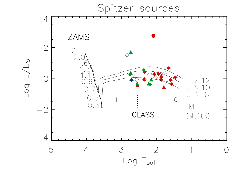
Figure 8: Bolometric Luminosity-Temperature diagram obtained for the Spizer ON-cloud YSOs. By using the classification criteria based on the MIR spectral slope red symbols correspond to Class I, green is used for FS, and blue for Class II sources. Different symbols denote different FIR spectral coverage: the filled circle is an object with with Herschel-SPIRE fluxes as well as 24 $\mu$m and 1.2 mm fluxes. Diamonds denote sources with 24 $\mu$m flux but undetected at 1.2 mm, with (filled) and without (open) Herschel-SPIRE fluxes, respectively. Finally triangles are objects without 1.2 mm flux and at least two fluxes in the 70–500 $\mu$m range, but with (filled) and without (open) 24 $\mu$m flux, respectively. Evolutive tracks are taken from Myers et al. (1998) and are labeled with the final stellar mass and the initial temperature of the outer envelope. In the bottom, with dashed lines, the correspondence between T_bol and spectral class as defined by Chen et al. (1995) is reported for comparison. The boundaries of the FS sources as suggetsed by Evans II et al. (2009) are also reported with dotted lines.

The result of this procedure is presented in Figure 8 where the bolometric luminosities and temperatures, computed for the 33 ON-cloud sources satisfying the preceding criteria, are shown superposed on some evolutionary tracks taken from Myers et al. (1998). In the bottom of this figure we also report the correspondence between T_bol and the evolutive classes suggested by Chen et al. (1995) and Evans II et al. (2009). It is noteworthy that the VMR-D cloud shows a relatively large number of sources (7 out of 33) that, classified as Class I (6 sources) and FS (1 source) according to their spectral slope in the MIR spectral range, show however T${}_{\mathrm{bol}}<70$ K suggesting instead that they could well be Class 0 objects as far as the bolometric temperature is concerned. This result confirms that the Spitzer sensitivity is sufficient to detect at least some of the Class 0 objects (Dunham et al., 2014) and in fact we find that in the VMR-D region $\sim 20$% of the Spitzer selected protostars can well be Class 0 sources.

5.2 Herschel selected sources

Herschel observations are more sensitive to the early protostellar phases (see, e.g., Stutz et al., 2013) and then give us the opportunity to complete our information on the early objects. In this perspective the bolometric temperature and luminosity for the 30 protostellar and the 92 starless Herschel ON-cloud sources have been computed by using the merged FIR catalog described in section 2.2. However, this catalog also includes complementary fluxes in the MIR spectral range so that we always use all the available fluxes, that for the ON-cloud protostars are reported in Table 6, to obtain the source luminosities. The resulting luminosity distribution is shown in the right panel of Figure 7 where a trend is apparent for the protostars to be, on average, more luminous than the starless cores. As expected, an opposite trend can be seen in the size distribution shown in the left panel where the protostellar sources appear as more compact objects with respect to the starless ones.

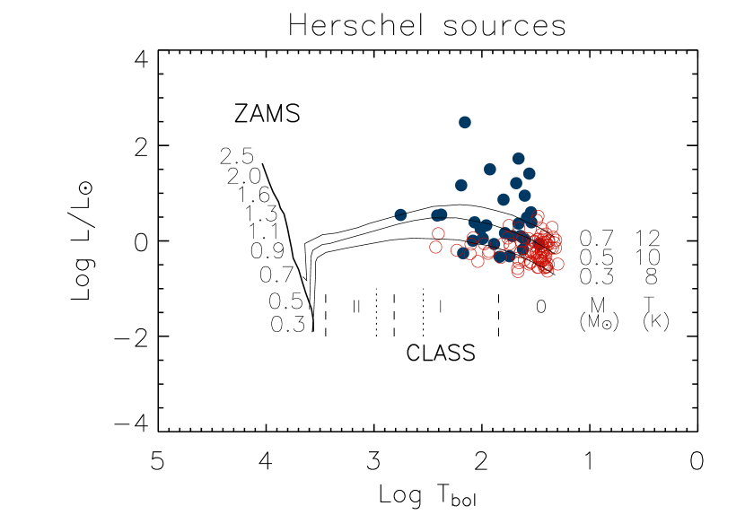
Figure 9: Bolometric Luminosity-Temperature diagram obtained for sources detected by Herschel. Filled blue circles are used for protostars, while open red circles represent starless sources. The statistics of the protostars is summarized in Table 4, their fluxes in Table 6, and their positions in the VMR-D cloud are shown in Figure 1. Ten protostars, listed in Table 7, are in common with Fig. 8.

By computing the bolometric temperatures from Equation (3) we also obtain the corresponding luminosity-temperature diagram that is shown in Figure 9. It can be directly compared with Figure 8 because both refer to the same region of the VMR-D, namely the intersection between the Herschel coverage, the Spitzer-PSC catalog, and the ON-cloud region that is shown in Figure 1. In the same figure the positions of both the Spitzer and Herschel selected sources are also shown.

Among these Herschel selected protostars we also find cases with T${}_{\mathrm{bol}}~{}<~{}70$ K that can be classified as Class 0 objects, even though in this case they are relatively more abundant (17 out of 30 protostars) than in the Spitzer selected sample. This is clearly as expected because the earlier phases, corresponding to colder objects, are more easily detected at the longer wavelengths of the Herschel observations.

It is however noteworthy that 10 out of the 30 Herschel protostars are also detected by Spitzer so that the total number of protostars in this region amounts to 53 sources. We then find that the Herschel observations are necessary to reveal 20 new protostars, corresponding to approximately one third of the total population in the surveyed part of the VMR-D cloud.

For the protostars in common, in Table 7 we report the classification determined by using the two schemes parameterized by the MIR spectral slope (Lada, 1987) and by the bolometric temperature (Chen et al., 1995; Evans II et al., 2009), respectively.

Considering now that the angular extension of our ON-cloud investigated region is $\sim 0.48$ deg² and that we adopted a nominal distance of 700 pc for the VMR-D, we find a protostellar surface density of $\sim 0.7$ pc^-2. A comparison with the star formation scaling law derived by Lombardi et al. (2013) for the Orion molecular cloud suggests that the VMR-D protostellar density would be compatible with a visual extinction $A_{V}\sim 5.5$, a value we find inside our ON-cloud region delimited by $A_{V}\sim 3.5$.

6 Discussion

A preliminary analysis of the young stellar population in the VMR-D cloud was presented in Paper I, but limited to the sources detected in all the four Spitzer-IRAC bands. Now, considering the full sample of the Spitzer-PSC sources and adopting a more demanding selection procedure, we obtain a more complete and reliable set of candidate YSOs to derive more accurate global properties of the SF in this cloud. Table 8 summarizes our results and, for the sake of comparison, also reports the results obtained by Evans II et al. (2009) for the SF regions of the c2d Spitzer legacy program. The comparison with Paper I shows that, despite the addition of sources detected in only three or even two IRAC bands, the number of FS and Class II candidate YSOs is similar as a result of adopting more stringent criteria to reject reddened photospheres in the selection pipeline (see Tab. 2 and Fig. 2). On the other hand, we select more Class I objects because a significant number of additional sources, detected in three or two IRAC bands, cannot be fitted by reddened photospheres and pass all the subsequent color-color and color-magnitude selection criteria discussed in Section 3. These are mainly sources detected at 3.6 and 4.5 $\mu$m, namely in the two more sensitive IRAC bands that are approximately ten times more sensitive than the 5.8 and 8.0 $\mu$m bands. The flux distribution of these additional sources peaks around 0.1 mJy showing that at these wavelengths they are faint objects near the completeness limit of the Spitzer-PSC catalog (see Tab. 1). Note however that, for the sake of a robust detection, these sources have been included in our analysis only if they also show a MIPS 24 $\mu$m counterpart.

Similarly, the number of Class III objects is noticeably larger than that quoted in Paper I. In this case the additional sources are mainly detected only in the first three IRAC bands. Despite a large fraction of these three-band sources are actually discarded as reddened photospheres, a still consistent number survive our selection steps, showing fluxes brighter than 0.1 mJy with a distribution peaking at 0.4, 0.3, and 0.25 mJy in the first three IRAC bands, respectively. In this respect we must consider that the VMR-D line of sight crosses the Galactic plane and thus is particularly contamined by giant stars that, because of their thin dust envelopes, can closely mimic a Class III SED, making it difficult to distinguish them from genuine YSOs. In this respect we recall that also the 8 $\mu$m PAH emission, which can be produced in carbon rich red giant envelopes as well as in blob of nebulosity, could bias the selection of Class III sources in particular for the faint objects. Despite our efforts to mitigate this problem by adopting appropriate color constraints in Section 3 and by subtracting the surface density of the YSOs seen outside the cloud (see Table 3), we consider that the number of Class III sources quoted in Table 3 and 8 is the most uncertain.

6.1 Comparison with other SFRs

To compare the relative abundance of the different classes in VMR-D with those characterizing other SFRs, we show in Figure 10 the number ratios for Class I, FS, and Class II sources obtained in the different studies based on Spitzer observations, along with their uncertainties evaluated by assuming Poisson statistics. In this diagram the Class I/FS ratio for the VMR-D is well in the range of the other SFRs, while the ratio (ClassI+FS)/Class II appears clearly displaced toward the largest values. A possible sistematic shift in this diagram could be produced by the interstellar reddening that tends to steepen the spectral slope and then to produce a bias in the classification favouring the earlier classes. However, reasonable values of the interstellar extinction toward VMR-D do not significantly influence the position in this diagram as is shown by the arrow in Figure 10 that represents the effect of an interstellar extinction A${}_{\mathrm{V}}=5$ mag. Given the values estimated for the insterstellar extinction toward VMR-D (A${}_{\mathrm{V}}\sim 2$mag, Cambresy, 1999; Joshi, 2005) we find that the offset position of the VMR-D in this diagram cannot be explained by this effect and then more probably reflects an intrinsic difference in the relative populations. That this can be the case is also shown by the work of Hsieh & Lai (2013) who noted that the relative number of the YSOs in Perseus significantly change if one considers the whole region or, separately, the two subregions extending eastward and westward of the R.A.=54^∘.3. To illustrate this point in Figure 10 we also report these two subregions as EPer and WPer, in this way showing how they diverge from the position occupied by the Perseus considered as a whole.

Intuitively we can guess that, in terms of a single SF burst, early objects are initially favoured so that both Class I/FS and (Class I+FS)/Class II number ratios should be relatively high. The absolute value and the time dependence expected for these ratios are clearly related to the specific modeling of the physical processes involved. Here we can only say that, if the position in this diagram has an evolutionary meaning, the VMR-D cloud appears much more similar to WPer and Ophiucus than to the other SFRs. However, if the SF occurs in multiple episodes or proceeds as a continuous process, Figure 10 cannot be easily interpreted and theoretical modeling is decisive to disentagle the different effects, a matter that is however beyond the scope of the present work.

This simplified analysis suffers however at least two limits that should be considered in future work: the possibility that Class II reddened disks can appear as FS sources (Dunham et al., 2014) and the presence, among the Class I objects, of cases that could well be Class 0 on the basis of their bolometric temperature. The first possibility tends to move the individual clouds toward the upper-left part of Figure 10 as could be the case for Ori, Mon, and CepOB3 whose FS sources have been selected by Kryukova et al. (2012) with criteria that are more restrictive than those used for the other SFRs. The second point on the possible presence of some Class 0 among the Class I objects should not change the significancy of the diagram as long as we simply reconsider that Class 0+I constitute a single counting bin. In this sense it is however noteworthy the larger relative content of protostars in VMR-D, WPer and Oph, suggesting for these regions a more recent SF event.

Once the YSOs are identified, further relevant quantities can be derived that characterize the SF in our cloud. These are reported in Table 9 and are obtained for a distance of 700 pc and under some simplifying assumptions as a mean mass of 0.5 M_☉, a binary fraction of 0.5, and an age of 2 Myr (Evans II et al., 2009), the latter being an estimate of the time taken to pass through the Class II SED phase. It is interesting that, as for the position of the VMR-D in Figure 10, we also find a greater similarity of the SF rate value to that of the Ophiucus cloud than to those of the other SFRs.

6.2 Protostellar luminosity function

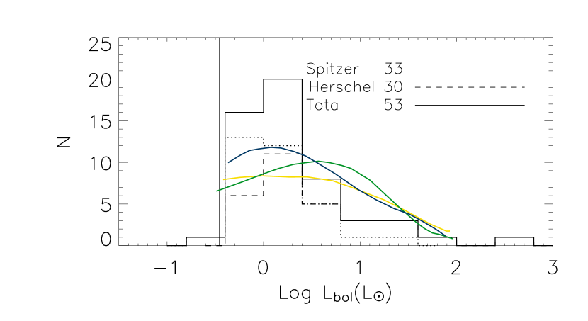
Figure 11: PLF: Spitzer (dotted line) and Herschel (dashed line) protostars located in the Spitzer/Herschel overlap region of VMR-D (see Fig. 1) and projected ON-cloud. The total luminosity function is shown with a solid line accounting for 10 objects that are common to the two samples. The vertical line represents the completeness limit based on the fluxes quoted in Table 1. Models from Offner & McKee (2011) including competitive accretion (yellow), turbulent core (green), and two component turbulent core model (blue), are also shown for comparison.

The PLF, determined by using all the protostars we find ON-cloud for which an accurate bolometric luminosity has been obtained in section 5, is shown in Figure 11. The completeness luminosity L${}_{\mathrm{com}}\simeq 0.35$ L_☉, shown as a vertical line, is evaluated on the basis of the completeness fluxes given in Table 1. In this figure we report only sources located ON-cloud in the overlap region observed by both Spitzer and Herschel, so that a comparison is possible between the ability of the two approaches to detect protostars. In particular we select 33 Spitzer and 30 Herschel protostellar sources respectively so that, considering that 10 sources are present in both samples, we conclude that in this region the Herschel observations contribute 20 additional protostars to those detected by Spitzer, leading up to 53 objects the total number of protostars. Taken all together these produce a more complete and representative PLF that is shown in the same Figure 11 with a continuous line. In the same figure three curves are also superimposed representing the PLF expected, after 1 Myr evolution, by models considering competitive accretion, turbulent core, and two component turbulent core, computed by Offner & McKee (2011) with an upper limit for the final stellar mass of 3 M_☉.

A comparison with the PLF already known for other clouds suggests that the high luminosity tail extending beyond 100 L_☉ makes the PLF in VMR-D more similar to those found in the high mass SFRs (Kryukova et al., 2012). The most luminous source, namely 42629 in the Spitzer-PSC numbering, is a Class I in both classification schemes, based on the MIR spectral slope and the bolometric temperature, and is located in the center of a bright IR cluster (IRS17, Liseau et al., 1992; Massi et al., 2000). A more quantitative comparison with the luminosity distribution obtained in other SFRs is presented in Table 10 that summarizes simple statistics corresponding to high and low-mass cases. The tabulated values suggest that the PLF in the VMR-D is more similar to that exhibited by the high mass SFRs, especially after correction of the reddening effect. Note however that our luminosities have not been corrected for this effect because they are essentially associated to Class 0 and I objects whose luminosity is dominated by the FIR contribution and is only marginally affected by the extinction.

A much more important difference is due to the completeness luminosity that in our case is approximately ten times that quoted by Kryukova et al. (2012). These authors in fact, adopting a remarkable relationship they find between the bolometric and the MIR luminosity of the YSOs with $\alpha>0$, derive the bolometric luminosity for a large number of objects with a well sampled SED in the MIR, in this way exploiting the high sensitivity of Spitzer-MIPS 24 $\mu$m observations at the risk of an uncertain extrapolation. With this method they sensibly enlarge the number of sources useful to obtain a better coverage of the low luminosity tail of the distribution. In our case we adopt a more conservative approach and compute the bolometric luminosity of Spitzer selected sources only when at least two good quality FIR fluxes are actually observed in the 70–500 $\mu$m range, with the result of a larger completeness luminosity that is most probably the cause of the differences seen in Table 10.

6.3 Envelope masses

Because the PLF depends on both mass and time, its relationship to the initial mass function of the stars produced by the protostars is not straightforward. Ideally, one should know both the luminosity and the age of an object to infer its mass on the basis of some theoretical model. In principle, because the contributions to the observed luminosity come from a central object as well as from a surrounding disk and possibly an envelope, a detailed modeling of the global SED is to be used to disentangle the masses of the different components.

Nevetheless, in the early phases when the protostars appear as a Class 0/I, it is customary to simplify the problem of deriving the envelope mass by assuming that the FIR emission is optically thin and is then useful to trace the total envelope mass. In our case we could consider the subsample of the ON-cloud protostars with an observed 500 $\mu$m flux, assuming that this is produced in an optically thin regime and adopting for the dust temperature the value obtained by fitting the Herschel fluxes at $\lambda\geq 160\mu$m (see Section 3) with the model in Equation (1). However, given that most of our sources are resolved at Herschel wavelengths we can also obtain the masses following the derivation in Pezzuto et al. (2012) that involves the angular extension $\Omega$ of the emitting body:

$$M=\frac{D^{2}~{}\Omega}{k_{\mathrm{ref}}}\left(\frac{\lambda_{0}}{\lambda_{\mathrm{ref}}}\right)^{2}$$ (5)

This expression allows us to derive the envelope mass for the 30 Herschel protostars (including the 7 cases without a 500 $\mu$m flux, see Table 6) because it does not depends explicitely on the observed flux at a given wavelength. This dependence is hidden in the fitting of the observed FIR fluxes with Equation (1) that gives also, as a by-product, the $\lambda_{0}$ value, namely the wavelength at which $\tau$=1. Similarly, we also extend this same approach to the starless cores detected in at least three Herschel wavelengths at $\lambda\geq 160~{}\mu$m.

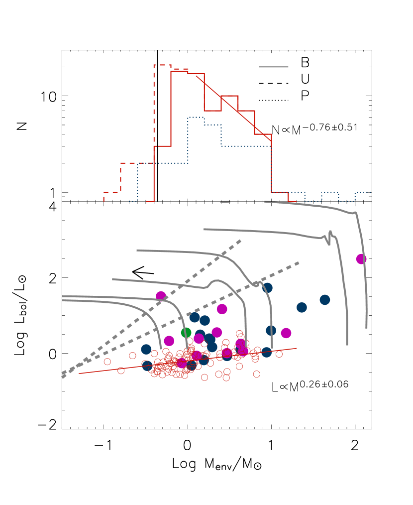
Figure 12: Upper panel: mass distribution for starless and protostellar Herschel sources detected ON-cloud. The red lines refer to the starless sources that are subdivided in unbound (dashed) and bound (solid) cases. The dotted blue line indicates the protostellar sources of Table 6, while the vertical solid line is the completeness limit implied by the photometry limits in Table 1. Lower panel: L_bol vs M_env diagram: filled and open circles represent protostars and starless cores, respectively. Protostars classified as Class 0, I, and Flat Spectrum in Table 4, are indicated with blue, magenta, and green filled circles, respectively. The superimposed grey lines represent the evolutionary tracks computed for different initial envelope masses by Molinari et al. (2008) to follow the path of a protostar in this diagram. The rising part corresponds to the main accretion phase ending with the transition region between Class 0 and Class I objects. This region is delimited by the two dashed lines taken from André et al. (2000) that ideally separate objects with M${}_{\mathrm{env}}>$ M_⋆ (lower) from those with M${}_{\mathrm{env}}<$ M_⋆ (upper). The arrow shows the evolutionary direction and the red straight line is a linear fit to the starless sources.

The envelope masses have been then obtained adopting an emission coefficient $k_{\mathrm{ref}}$=0.1 cm² g^-1 of gas mass at $\lambda_{\mathrm{ref}}$=250 $\mu$m (Hildebrand, 1983; Suutarinen et al., 2013) and a scaling law $k=k_{\mathrm{ref}}(\lambda_{\mathrm{ref}}/\lambda)^{2}$. In Figure 12 we present the resulting distribution of the envelope masses (upper panel) computed for both protostellar and starless sources. Because in the latter case the derived values represent the true total mass, it is interesting to compare the derived masses with the Bonnor-Ebert critical mass approximately given by $M_{\mathrm{BE}}\approx 2.4~{}R_{\mathrm{BE}}~{}a^{2}/G$, with $a$ being the sound speed at the source temperature. Such a comparison offers a simple way to separate prestellar from quiescent cores by simply assuming that masses M $\gtrsim 0.5$ M_BE are bound and then should be considered as prestellar because they more probably evolve toward a protostar.

Assuming for $R_{\mathrm{BE}}$ the observed deconvolved radius at 250 $\mu$m we find that $M>0.5M_{\mathrm{BE}}$ for 67 out of 92 ON-cloud sources that we then consider as bound and potentially prestellar. In Figure 12 the distribution of all the starless sources is shown as a dashed red line that merges, at $M>1M_{\sun}$, in the continuous red line corresponding to the prestellar component, suggesting that all the cores more massive that the solar mass are prestellar. Considering poissonian uncertainties and varying the binsize in reasonable limits ( 10% around a bin size=0.2) we obtain for masses $M>1M_{\sun}$ a slope of -0.76$\pm$0.51 where the uncertainty is dominated by the poor statistics. Even if this value is lower than that found in Vela-C molecular cloud by Giannini et al. (2012) and in the outer Galaxy by Elia et al. (2013), given the large uncertainty involved we cannot claim for meaningful differences.

In the same figure we also show (bottom panel) the L_bol vs M_env diagram for the VMR-D protostars with superimposed the evolutive tracks computed by Molinari et al. (2008) for different initial envelope masses. For comparison we also report the starless sources noting that they populate the low luminosity part of the diagram and show a relatively smaller luminosity spread with respect to the protostars. A linear fit to their distribution in this diagram give a slope that is shallower than that found in both Vela-C (Giannini et al., 2012) and the third Galactic quadrant (Elia et al., 2013), suggesting possible differences in the clump/core forming mechanism. On the other hand the protostars are more widely distributed in this diagram, the most of them being located on the rising branch of the evolutionary tracks corresponding to the main accretion phase. Following André et al. (2000) we also report in this diagram two lines that delimit what is thought to be the transition zone separating the low luminosity branch in which M${}_{\mathrm{env}}>$ M_⋆, generally associated to the Class 0 phase, from the region in which M${}_{\mathrm{env}}<$ M_⋆ corresponding to the Class I and later phases. Remarkably, in most cases the protostars fall below the transition region suggesting a very recent star formation episode. However a similar distribution of the protostars is also seen in other SFR observed with Herschel (Giannini et al., 2012; Elia et al., 2013) and this seems to be unrealistic, raising a problem of consistency with the model. From an observational point of view, one possibility is that, due to our need to know at least three fluxes at $\lambda\geq 160~{}\mu$m to appropriately fit a modified blackbody, we introduce a selection effect favouring the earliest objects, a point that should be better considered in future work.

7 Conclusions

In this work we have studied the YSO population in the VMR-D cloud by exploiting both the Spitzer-PSC catalog, obtained from Spitzer observations and published in Paper I, and the recent Herschel observations carried out during the completion of the Hi-GAL key program involving part of this region. The main results can be summarized as follows:

• A list of 1470 candidate YSOs, identified out of the $\sim$170,000 Spitzer-PSC catalog sources, has been obtained through a selection pipeline designed to exclude reddened normal stars, as well as Galactic and extragalactic contaminants.

• YSOs have been subdivided in classes according to their spectral slope in the near-mid IR and their relative numbers (86, 53, 136, and 282 for Class I, FS, II, and III, respectively), obtained after subtraction of the estimated background population, have been compared with those characterizing other star forming clouds showing that the YSO content in VMR-D is similar to that seen in Ophiucus and in the western part of Perseus.

• The Spitzer-PSC catalog has been complemented to obtain the largest data set on the continuum spectrum of the sources, including fluxes from the 2MASS and WISE public surveys as well as from new Herschel FIR observations and previous 1.2 mm SEST-SIMBA continuum mapping of the VMR-D region.

• The Herschel/Hi-GAL maps ($\lambda=70$, 160, 250, 350,$\mathrm{and}~{}500~{}\mu$m) overlapping our VMR-D region have been first used to identify the ON-cloud regions delimited by a column density N(H₂)=6.5$\times 10^{21}$ cm^-2 and then analyzed to obtain a merged catalog of compact FIR sources useful for searching additional protostars undetected by Spitzer. This catalog, complemented with fluxes coming from the Spitzer-PSC catalog as well as from WISE and the 1.2 mm catalog, has been exploited to find and characterize 30 protostellar and 92 starless sources and to evaluate their bolometric luminosities and temperatures.

• Bolometric luminosities and temperatures have been also obtained for 33 Spitzer selected ON-cloud protostars. These have been plotted in a $L_{\mathrm{bol}}$ vs $T_{\mathrm{bol}}$ diagram showing that 7 (six Class I, and one FS) out of these 33 protostars can actually represent Class 0 objects due to their low bolometric temperature (T${}_{\mathrm{bol}}<$70 K).

• The distribution of the luminosities of both the Spitzer and Herschel selected protostars show a bright outlier, corresponding to the same object Spitzer-PSC 42629 (IRS17 in Liseau et al., 1992), suggesting that VMR-D is also forming relatively high mass objects.

• The complete PLF of the ON-cloud region covered by both Spitzer and Herschel observations has been obtained by merging together the 33 Spitzer and the 30 Herschel selected protostars. Given that 10 objects are in both samples we count a total of 53 objects and find that Spitzer is able to detect approximately two-thirds of the protostellar population actually present in VMR-D. This stresses the need for using also the Herschel observations in studying the earlier protostellar phases.

• The envelope masses have been obtained for all the Herschel protostellar sources detected ON-cloud and for which an envelope temperature can be determined. A plot of the masses versus the corresponding luminosities shows that, by comparison with evolutive tracks, we are mainly sampling objects in the main accretion phase. A possibility is that a selection effect is implied by our preference for sources also detected in the FIR, a choice that is dictated by the need to obtain accurate bolometric quantities.

Table 1: Catalogs considered.

Name	2MASS	WISE	Spitzer-IRAC+MIPS	Herschel	SEST-SIMBA
Band	J H K	3.4 4.6 12 22	3.6 4.5 5.8 8.0 24 70	70 160 250 350 500	1200
Beam size (″)	2.5 – 3	6 – 12	1.7 – 6	7.6 12.3 18 25 36	24
Association radius (″)	0.6	0.9	1	4 8 11 16 21	12
Completeness flux (mJy)	0.76 1.23 1.67	4.9 2.7 3.2 5.3	0.05 0.05 0.29 0.4 2.0 500	1800 1100 600 600 600	20
Reference	1	2	3	4	5

Table 2: Spitzer Source counts through the selection pipeline.

Step	1234	123X	12X4	1X34	X234	XX34	1XX4	12XX	1X3X	X2X4	Total
0: first selection	8852(436)	7210(28)	151(12)	19(12)	30(19)	9(9)	1(1)	116(116)	2(2)	1(1)	16391
1: reddened stars	-6110	-6063	-9	-10	-15	-6	0	-3	0	-1	-12217
2: Har07 criteria	-2059	0	-142	0	-15	0	-1	0	0	0	-2217
3: Gut09 criteria	-17	-467	0	0	0	0	0	0	0	0	-484
4: undefined slope	-9	-3	0	0	0	0	0	0	0	0	-12
Total	657	677	0	9	0	3	0	113	2	0	1461

Table 3: VMR-D Statistics of the Spitzer YSOs (MIR catalog).

Region	ON	OFF	OUT	TOT	ON-OFF
$\Omega$(deg2) $\rightarrow$	0.54	0.52	0.14	1.20	0.54
Class I	105(12%)	22	22	149	82$\pm$ 11 (15%)
Flat spectrum	58 (7%)	6	9	73	52$\pm$ 8 (10%)
Class II	171(20%)	40	33	244	129$\pm$ 14 (24%)
Class III	535(61%)	288	181	1004	236$\pm$ 28 (51%)

Table 4: VMR-D Statistics of the Herschel protostars (FIR catalog).

Region	ON	OFF
$\Omega$(deg2) $\rightarrow$	0.48	0.33
Class 0	17	$\cdots$
Class I	12	1
Flat Spectrum	1	$\cdots$

Table 5: Photometry of the Spitzer selected protostars

ID	PSC	RA	DEC	$F_{J}\pm\Delta F_{J}$	$F_{H}\pm\Delta F_{H}$
$F_{K}\pm\Delta F_{K}$	$F_{W1}\pm\Delta F_{W1}$	$F_{W2}\pm\Delta F_{W2}$	$F_{W3}\pm\Delta F_{W3}$	$F_{W4}\pm\Delta F_{W4}$	$F_{3.6}\pm\Delta F_{3.6}$
$F_{4.5}\pm\Delta F_{4.5}$	$F_{5.8}\pm\Delta F_{5.8}$	$F_{8.0}\pm\Delta F_{8.0}$	$F_{24}\pm\Delta F_{24}$	$F_{70}\pm\Delta F_{70}$	$F_{160}\pm\Delta F_{160}$
$F_{250}\pm\Delta F_{250}$	$F_{350}\pm\Delta F_{350}$	$F_{500}\pm\Delta F_{500}$	$F_{1200}\pm\Delta F_{1200}$
1	8036	131.28840	-43.63255	$\cdots$	$\cdots$
$\cdots$	0.00016 $\pm$ 0.00005	0.00025 $\pm$ 0.00009	0.0027 $\pm$ 0.0003	0.0165 $\pm$ 0.0013	0.000040 $\pm$ 0.000004
$\cdots$	$\cdots$	$\cdots$	0.017 $\pm$ 0.003	$\cdots$	1.09 $\pm$ 0.08
2.70 $\pm$ 0.06	3.08 $\pm$ 0.08	1.63 $\pm$ 0.06	$\cdots$
2	10558	131.31710	-43.86800	0.000682 $\pm$ 0.000057	0.000835 $\pm$ 0.000088
0.00076 $\pm$ 0.00010	$\cdots$	$\cdots$	$\cdots$	$\cdots$	0.00069 $\pm$ 0.00003
0.00042 $\pm$ 0.00001	$\cdots$	$\cdots$	0.0361 $\pm$ 0.0053	$\cdots$	2.71 $\pm$ 0.03
$\cdots$	$\cdots$	$\cdots$	$\cdots$
3	17534	131.38797	-43.82994	0.051 $\pm$ 0.01	0.136 $\pm$ 0.004
0.29 $\pm$ 0.01	0.82 $\pm$ 0.05	0.94 $\pm$ 0.04	1.97 $\pm$ 0.02	9.01 $\pm$ 0.07	0.58 $\pm$ 0.02
0.60 $\pm$ 0.02	0.68 $\pm$ 0.02	1.08 $\pm$ 0.02	1.93 $\pm$ 0.26	25.5 $\pm$ 2.5	$\cdots$
$\cdots$	$\cdots$	32.3 $\pm$ 0.1	$\cdots$
4	19124	131.40512	-43.31155	0.00099 $\pm$ 0.00006	0.0199 $\pm$ 0.0005
0.158 $\pm$ 0.003	1.44 $\pm$ 0.15	4.6 $\pm$ 0.7	2.12 $\pm$ 0.03	1.36 $\pm$ 0.03	1.13 $\pm$ 0.05
1.87 $\pm$ 0.08	2.44 $\pm$ 0.04	2.59 $\pm$ 0.07	0.94 $\pm$ 0.15	0.49 $\pm$ 0.01	$\cdots$
$\cdots$	$\cdots$	$\cdots$	$\cdots$
5	19667	131.41093	-43.91746	$\cdots$	0.0023 $\pm$ 0.0002
0.0089 $\pm$ 0.0003	0.0233 $\pm$ 0.0005	0.0405 $\pm$ 0.0007	0.062 $\pm$ 0.001	0.259 $\pm$ 0.005	0.0263 $\pm$ 0.0007
0.0326 $\pm$ 0.0014	0.0419 $\pm$ 0.0008	0.050 $\pm$ 0.001	0.194 $\pm$ 0.008	0.48 $\pm$ 0.02	4.04 $\pm$ 0.03
16.70 $\pm$ 0.26	7.29 $\pm$ 0.07	4.79 $\pm$ 0.08	$\cdots$
6	21825	131.43290	-43.45194	$\cdots$	$\cdots$
$\cdots$	0.00162 $\pm$ 0.00005	0.0088 $\pm$ 0.0002	0.053 $\pm$ 0.001	0.411 $\pm$ 0.006	0.0120 $\pm$ 0.0005
0.027 $\pm$ 0.001	0.053 $\pm$ 0.002	0.082 $\pm$ 0.002	0.361 $\pm$ 0.006	1.96 $\pm$ 0.02	1.98 $\pm$ 0.04
$\cdots$	$\cdots$	$\cdots$	$\cdots$
7	22262	131.43750	-43.44786	$\cdots$	$\cdots$
0.0021 $\pm$ 0.0001	0.00712 $\pm$ 0.00015	0.01389 $\pm$ 0.00026	0.0250 $\pm$ 0.0008	0.1386 $\pm$ 0.0034	0.00544 $\pm$ 0.00017
0.007139 $\pm$ 0.000290	0.011046 $\pm$ 0.000435	0.013362 $\pm$ 0.000505	0.000587 $\pm$ 0.000000	$\cdots$	0.659356 $\pm$ 0.000453
$\cdots$	$\cdots$	$\cdots$	$\cdots$
8	23011	131.44509	-43.38967	$\cdots$	$\cdots$
$\cdots$	$\cdots$	$\cdots$	$\cdots$	$\cdots$	0.000487 $\pm$ 0.000025
0.00157 $\pm$ 0.00007	0.00310 $\pm$ 0.00009	0.00297 $\pm$ 0.00009	0.0579 $\pm$ 0.0015	0.71 $\pm$ 0.02	0.86 $\pm$ 0.03
2.08 $\pm$ 0.02	2.12 $\pm$ 0.05	2.09 $\pm$ 0.06	$\cdots$
9	24056	131.45576	-43.88890	$\cdots$	0.00081 $\pm$ 0.00009
0.0020 $\pm$ 0.0001	$\cdots$	$\cdots$	$\cdots$	$\cdots$	0.0033 $\pm$ 0.0001
0.0043 $\pm$ 0.0002	$\cdots$	$\cdots$	0.056 $\pm$ 0.001	0.432 $\pm$ 0.014	2.66 $\pm$ 0.02
10.16 $\pm$ 0.08	4.36 $\pm$ 0.04	8.84 $\pm$ 0.08	$\cdots$
10	26276	131.47872	-43.91127	0.00116 $\pm$ 0.00009	0.0028 $\pm$ 0.0002
0.0049 $\pm$ 0.0002	0.0064 $\pm$ 0.0001	0.0066 $\pm$ 0.0001	0.0064 $\pm$ 0.0003	0.021 $\pm$ 0.002	0.0052 $\pm$ 0.0005
0.0055 $\pm$ 0.0005	0.0048 $\pm$ 0.0003	0.0044 $\pm$ 0.0002	0.0226 $\pm$ 0.0007	$\cdots$	$\cdots$
2.84 $\pm$ 0.07	1.44 $\pm$ 0.04	0.940 $\pm$ 0.015	$\cdots$
11	37210	131.58937	-43.66819	$\cdots$	0.00026 $\pm$ 0.00009
0.00067 $\pm$ 0.00009	0.00068 $\pm$ 0.00002	0.00180 $\pm$ 0.00004	0.0011 $\pm$ 0.0002	0.0183 $\pm$ 0.0011	0.00165 $\pm$ 0.00004
0.00200 $\pm$ 0.00007	0.00210 $\pm$ 0.00008	0.00212 $\pm$ 0.00006	0.0154 $\pm$ 0.0006	$\cdots$	$\cdots$
1.63 $\pm$ 0.03	2.42 $\pm$ 0.03	0.52 $\pm$ 0.04	$\cdots$
12	38922	131.60656	-43.90894	0.00074 $\pm$ 0.000078	0.0030 $\pm$ 0.0001
0.0061 $\pm$ 0.0002	0.0121 $\pm$ 0.0003	0.0210 $\pm$ 0.0004	0.0367 $\pm$ 0.0008	0.160 $\pm$ 0.004	0.0132 $\pm$ 0.0003
0.0193 $\pm$ 0.0005	0.0262 $\pm$ 0.0005	0.0374 $\pm$ 0.0008	0.1066 $\pm$ 0.0046	$\cdots$	1.76 $\pm$ 0.02
$\cdots$	$\cdots$	$\cdots$	$\cdots$
13	39571	131.61333	-43.91638	$\cdots$	0.00113 $\pm$ 0.00010
0.0020 $\pm$ 0.0001	$\cdots$	$\cdots$	$\cdots$	$\cdots$	0.00164 $\pm$ 0.00004
0.00158 $\pm$ 0.00007	0.00131 $\pm$ 0.00004	0.00091 $\pm$ 0.00006	$\cdots$	$\cdots$	6.95 $\pm$ 0.04
12.08 $\pm$ 0.07	$\cdots$	$\cdots$	$\cdots$
14	39589	131.61359	-43.71115	$\cdots$	$\cdots$
$\cdots$	$\cdots$	$\cdots$	$\cdots$	$\cdots$	0.00147 $\pm$ 0.00004
0.00213 $\pm$ 0.00005	0.00290 $\pm$ 0.00006	0.0042 $\pm$ 0.0001	0.121 $\pm$ 0.004	3.19 $\pm$ 0.01	6.97 $\pm$ 0.05
21.65 $\pm$ 0.13	9.95 $\pm$ 0.07	5.31 $\pm$ 0.55	$\cdots$
15	41657	131.63487	-43.54801	$\cdots$	$\cdots$
$\cdots$	$\cdots$	$\cdots$	$\cdots$	$\cdots$	0.000027 $\pm$ 0.000002
0.000030 $\pm$ 0.000002	$\cdots$	$\cdots$	0.0201 $\pm$ 0.0005	$\cdots$	0.584 $\pm$ 0.009
1.48 $\pm$ 0.02	2.17 $\pm$ 0.03	2.03 $\pm$ 0.02	$\cdots$
16	42629	131.64522	-43.90839	$\cdots$	0.0092 $\pm$ 0.0007
0.093 $\pm$ 0.003	0.966 $\pm$ 0.056	4.8 $\pm$ 0.6	14.7 $\pm$ 0.1	84.7 $\pm$ 0.2	0.85 $\pm$ 0.03
1.87 $\pm$ 0.07	3.67 $\pm$ 0.11	3.4 $\pm$ 0.6	$>$ 4	458.6 $\pm$ 2.7	356.4 $\pm$ 1.8
458.6 $\pm$ 8.0	249.8 $\pm$ 1.7	116.3 $\pm$ 0.6	8.79
17	47368	131.69429	-43.33628	$\cdots$	$\cdots$
0.00088 $\pm$ 0.00010	0.00200 $\pm$ 0.00005	0.00424 $\pm$ 0.00008	0.0166 $\pm$ 0.0004	0.0585 $\pm$ 0.0031	0.00373 $\pm$ 0.00008
0.0056 $\pm$ 0.0001	0.0085 $\pm$ 0.0002	0.0125 $\pm$ 0.0002	$\cdots$	$\cdots$	0.320 $\pm$ 0.004
1.357 $\pm$ 0.008	1.626 $\pm$ 0.015	$\cdots$	$\cdots$
18	47436	131.69495	-43.88731	$\cdots$	$\cdots$
$\cdots$	0.00095 $\pm$ 0.00003	0.00333 $\pm$ 0.00007	0.0156 $\pm$ 0.0003	0.251 $\pm$ 0.005	0.00163 $\pm$ 0.00006
0.0030 $\pm$ 0.0001	0.00370 $\pm$ 0.00008	0.00382 $\pm$ 0.00007	0.114 $\pm$ 0.002	0.780 $\pm$ 0.005	1.95 $\pm$ 0.01
$\cdots$	$\cdots$	$\cdots$	$\cdots$
19	48046	131.70117	-43.88612	$\cdots$	$\cdots$
$\cdots$	$\cdots$	$\cdots$	$\cdots$	$\cdots$	0.00098 $\pm$ 0.00002
0.00255 $\pm$ 0.00006	0.00409 $\pm$ 0.00009	0.00522 $\pm$ 0.00008	0.114 $\pm$ 0.007	1.83 $\pm$ 0.02	3.63 $\pm$ 0.04
$\cdots$	$\cdots$	$\cdots$	$\cdots$
20	50748	131.72791	-43.87676	$\cdots$	$\cdots$
0.00068 $\pm$ 0.00009	0.00199 $\pm$ 0.00009	0.0082 $\pm$ 0.0002	0.0297 $\pm$ 0.0007	0.131 $\pm$ 0.004	0.0053 $\pm$ 0.0001
0.0114 $\pm$ 0.0003	0.0212 $\pm$ 0.0004	0.0298 $\pm$ 0.0005	0.154 $\pm$ 0.003	0.540 $\pm$ 0.012	0.754 $\pm$ 0.015
2.26 $\pm$ 0.04	$\cdots$	6.40 $\pm$ 0.02	$\cdots$
21	58569	131.80015	-43.37957	$\cdots$	$\cdots$
$\cdots$	0.00164 $\pm$ 0.00006	0.0083 $\pm$ 0.0002	0.0121 $\pm$ 0.0004	0.089 $\pm$ 0.003	0.0026 $\pm$ 0.0002
0.0070 $\pm$ 0.0005	0.0110 $\pm$ 0.0006	0.0133 $\pm$ 0.0007	0.089 $\pm$ 0.005	2.55 $\pm$ 0.03	2.43 $\pm$ 0.06
3.92 $\pm$ 0.20	3.70 $\pm$ 0.06	2.42 $\pm$ 0.02	$\cdots$
22	59696	131.80945	-43.30581	0.0033 $\pm$ 0.0001	0.0074 $\pm$ 0.0002
0.0113 $\pm$ 0.0004	0.0199 $\pm$ 0.0007	0.032 $\pm$ 0.001	0.051 $\pm$ 0.002	0.147 $\pm$ 0.007	0.0194 $\pm$ 0.0005
0.0286 $\pm$ 0.0008	0.034 $\pm$ 0.001	0.0409 $\pm$ 0.0008	0.27 $\pm$ 0.04	1.21 $\pm$ 0.04	2.50 $\pm$ 0.03
3.80 $\pm$ 0.03	1.94 $\pm$ 0.04	1.52 $\pm$ 0.02	$\cdots$
23	65153	131.85542	-43.81557	$\cdots$	$\cdots$
$\cdots$	$\cdots$	$\cdots$	$\cdots$	$\cdots$	0.0088 $\pm$ 0.0002
0.0183 $\pm$ 0.0006	0.0357 $\pm$ 0.0006	0.050 $\pm$ 0.001	0.49 $\pm$ 0.01	1.88 $\pm$ 0.02	2.90 $\pm$ 0.06
5.79 $\pm$ 0.03	3.02 $\pm$ 0.04	2.06 $\pm$ 0.04	$\cdots$
24	65982	131.86223	-43.45189	$\cdots$	0.00058 $\pm$ 0.00008
0.00235 $\pm$ 0.00012	0.00080 $\pm$ 0.00002	0.00294 $\pm$ 0.00005	0.00837 $\pm$ 0.00063	0.0456 $\pm$ 0.0023	0.00534 $\pm$ 0.00015
0.00807 $\pm$ 0.00015	0.0118 $\pm$ 0.0002	0.01596 $\pm$ 0.00022	0.0520 $\pm$ 0.0010	0.543 $\pm$ 0.004	$\cdots$
$\cdots$	$\cdots$	$\cdots$	$\cdots$
25	68231	131.88064	-43.89669	$\cdots$	$\cdots$
$\cdots$	0.00108 $\pm$ 0.00003	0.0068 $\pm$ 0.0001	0.0055 $\pm$ 0.0004	0.046 $\pm$ 0.002	0.00142 $\pm$ 0.00005
0.0044 $\pm$ 0.0001	0.0069 $\pm$ 0.0002	0.0068 $\pm$ 0.0002	0.042 $\pm$ 0.004	0.767 $\pm$ 0.005	2.66 $\pm$ 0.07
5.22 $\pm$ 0.03	2.78 $\pm$ 0.03	$\cdots$	$\cdots$
26	72151	131.91048	-43.82592	$\cdots$	$\cdots$
$\cdots$	0.00021 $\pm$ 0.00002	0.00063 $\pm$ 0.00002	$\cdots$	0.024 $\pm$ 0.002	0.00038 $\pm$ 0.00001
0.00047 $\pm$ 0.00002	0.00031 $\pm$ 0.00003	$\cdots$	0.0100 $\pm$ 0.0003	$\cdots$	1.19 $\pm$ 0.01
6.06 $\pm$ 0.03	5.54 $\pm$ 0.02	5.86 $\pm$ 0.02	$\cdots$
27	72976	131.91688	-43.43769	0.00047 $\pm$ 0.00005	0.00216 $\pm$ 0.00012
0.00415 $\pm$ 0.00015	$\cdots$	$\cdots$	$\cdots$	$\cdots$	0.00640 $\pm$ 0.00019
0.00621 $\pm$ 0.00012	0.00643 $\pm$ 0.00014	0.00568 $\pm$ 0.00010	$\cdots$	$\cdots$	4.409 $\pm$ 0.018
7.35 $\pm$ 0.65	8.95 $\pm$ 0.07	$\cdots$	$\cdots$
28	83949	131.99760	-43.65348	$\cdots$	$\cdots$
0.0011 $\pm$ 0.0001	0.00284 $\pm$ 0.00007	0.0056 $\pm$ 0.0001	$\cdots$	0.007 $\pm$ 0.002	0.0023 $\pm$ 0.0001
0.0032 $\pm$ 0.0002	0.0041 $\pm$ 0.0002	0.0043 $\pm$ 0.0001	0.0135 $\pm$ 0.0005	$\cdots$	1.44 $\pm$ 0.02
4.55 $\pm$ 0.02	3.07 $\pm$ 0.03	$\cdots$	$\cdots$
29	86208	132.01412	-43.85429	0.00275 $\pm$ 0.00012	0.00684 $\pm$ 0.00027
0.00938 $\pm$ 0.00031	0.01279 $\pm$ 0.00027	0.01784 $\pm$ 0.00033	0.0569 $\pm$ 0.0010	0.1436 $\pm$ 0.0038	0.01606 $\pm$ 0.00037
0.01977 $\pm$ 0.00066	0.02691 $\pm$ 0.00055	0.04102 $\pm$ 0.00059	0.1091 $\pm$ 0.0016	$\cdots$	3.11 $\pm$ 0.02
10.07 $\pm$ 0.06	5.43 $\pm$ 0.03	2.73 $\pm$ 0.02	$\cdots$
30	113290	132.22921	-43.71078	$\cdots$	$\cdots$
$\cdots$	$\cdots$	$\cdots$	$\cdots$	$\cdots$	0.000164 $\pm$ 0.000004
0.000104 $\pm$ 0.000004	$\cdots$	$\cdots$	0.0191 $\pm$ 0.0033	$\cdots$	0.461 $\pm$ 0.006
1.017 $\pm$ 0.02	1.44 $\pm$ 0.02	$\cdots$	$\cdots$
31	123062	132.32596	-43.93661	$\cdots$	$\cdots$
0.00069 $\pm$ 0.00009	0.00121 $\pm$ 0.00005	0.00227 $\pm$ 0.00005	0.0061 $\pm$ 0.0002	0.021 $\pm$ 0.001	0.00172 $\pm$ 0.00005
0.00246 $\pm$ 0.00005	0.00316 $\pm$ 0.00006	0.00331 $\pm$ 0.00005	0.0081 $\pm$ 0.0004	$\cdots$	0.777 $\pm$ 0.006
2.19 $\pm$ 0.20	$\cdots$	0.970 $\pm$ 0.007	$\cdots$
32	124358	132.33936	-44.03091	$\cdots$	$\cdots$
$\cdots$	$\cdots$	$\cdots$	$\cdots$	$\cdots$	0.00110 $\pm$ 0.00002
0.00208 $\pm$ 0.00007	0.00319 $\pm$ 0.00007	0.00455 $\pm$ 0.00008	$\cdots$	2.31 $\pm$ 0.03	3.52 $\pm$ 0.04
5.84 $\pm$ 0.04	4.32 $\pm$ 0.05	3.33 $\pm$ 0.08	$\cdots$
33	127425	132.37080	-43.99599	$\cdots$	$\cdots$
$\cdots$	$\cdots$	$\cdots$	$\cdots$	$\cdots$	0.00050 $\pm$ 0.00001
0.00054 $\pm$ 0.00002	0.00055 $\pm$ 0.00002	0.00052 $\pm$ 0.00001	$\cdots$	$\cdots$	0.899 $\pm$ 0.005
2.09 $\pm$ 0.06	2.02 $\pm$ 0.02	1.63 $\pm$ 0.02	$\cdots$

Table 6: Photometry of the Herschel selected protostars

ID	RA	DEC	$F_{W1}\pm\Delta F_{W1}$	$F_{W2}\pm\Delta F_{W2}$	$F_{W3}\pm\Delta F_{W3}$
$F_{W4}\pm\Delta F_{W4}$	$F_{3.6}\pm\Delta F_{3.6}$	$F_{4.5}\pm\Delta F_{4.5}$	$F_{5.8}\pm\Delta F_{5.8}$	$F_{8.0}\pm\Delta F_{8.0}$	$F_{24}\pm\Delta F_{24}$
$F_{BLUE}\pm\Delta F_{BLUE}$	$F_{RED}\pm\Delta F_{RED}$	$F_{PSW}\pm\Delta F_{PSW}$	$F_{PMW}\pm\Delta F_{PMW}$	$F_{PLW}\pm\Delta F_{PLW}$	$F_{1200}\pm\Delta F_{1200}$
1	131.18478	-43.70255	0.00221 $\pm$ 0.00005	0.00141 $\pm$ 0.00003	0.0025 $\pm$ 0.0004
0.046 $\pm$ 0.001	0.00053 $\pm$ 0.00004	0.00060 $\pm$ 0.00002	0.00067 $\pm$ 0.00003	0.00095 $\pm$ 0.00003	0.045 $\pm$ 0.001
0.35 $\pm$ 0.01	0.69 $\pm$ 0.01	1.51 $\pm$ 0.03	0.72 $\pm$ 0.09	0.49 $\pm$ 0.01	$\cdots$
2	131.28860	-43.63342	0.00016 $\pm$ 0.00001	0.00025 $\pm$ 0.00005	0.0027 $\pm$ 0.0003
0.0165 $\pm$ 0.0013	0.000044 $\pm$ 0.000003	0.00014 $\pm$ 0.00001	$\cdots$	0.000091 $\pm$ 0.000020	0.0171 $\pm$ 0.0007
0.63 $\pm$ 0.02	1.09 $\pm$ 0.02	2.70 $\pm$ 0.03	3.08 $\pm$ 0.04	1.63 $\pm$ 0.03	$\cdots$
3	131.39476	-43.85289	$\cdots$	$\cdots$	$\cdots$
$\cdots$	0.00175 $\pm$ 0.00008	0.00166 $\pm$ 0.00005	0.0041 $\pm$ 0.0002	0.0091 $\pm$ 0.0007	$\cdots$
19.4 $\pm$ 0.5	17.48 $\pm$ 0.44	40.6 $\pm$ 0.2	27.0 $\pm$ 0.1	$\cdots$	3.17
4	131.40118	-43.86400	$\cdots$	$\cdots$	$\cdots$
$\cdots$	0.0015 $\pm$ 0.0001	0.0016 $\pm$ 0.0001	0.0083 $\pm$ 0.0009	$\cdots$	$\cdots$
61.65 $\pm$ 0.17	76.48 $\pm$ 0.18	87.56 $\pm$ 0.60	93.30 $\pm$ 0.50	$\cdots$	3.70
5	131.41060	-43.91772	0.0233 $\pm$ 0.0005	0.0406 $\pm$ 0.0007	0.062 $\pm$ 0.001
0.259 $\pm$ 0.005	0.0263 $\pm$ 0.0007	0.033 $\pm$ 0.001	0.0420 $\pm$ 0.0008	0.050 $\pm$ 0.001	0.194 $\pm$ 0.008
0.483 $\pm$ 0.012	4.04 $\pm$ 0.03	16.70 $\pm$ 0.26	7.29 $\pm$ 0.07	4.79 $\pm$ 0.08	$\cdots$
6	131.42451	-43.86047	$\cdots$	$\cdots$	$\cdots$
$\cdots$	$\cdots$	$\cdots$	$\cdots$	$\cdots$	$\cdots$
8.70 $\pm$ 0.06	54.36 $\pm$ 0.35	120.98 $\pm$ 0.11	75.20 $\pm$ 0.19	$\cdots$	$\cdots$
7	131.42975	-43.45671	0.00322 $\pm$ 0.00007	0.0156 $\pm$ 0.0003	0.0076 $\pm$ 0.00062
0.0937 $\pm$ 0.0027	0.00240 $\pm$ 0.00009	0.0052 $\pm$ 0.0002	0.0076 $\pm$ 0.0003	0.0080 $\pm$ 0.0003	$\cdots$
0.623 $\pm$ 0.009	2.70 $\pm$ 0.05	6.82 $\pm$ 0.03	4.59 $\pm$ 0.05	3.87 $\pm$ 0.04	$\cdots$
8	131.44052	-43.43735	$\cdots$	$\cdots$	$\cdots$
$\cdots$	0.0026 $\pm$ 0.0002	0.0037 $\pm$ 0.0002	0.0044 $\pm$ 0.0002	0.0033 $\pm$ 0.0001	$\cdots$
0.399 $\pm$ 0.006	1.58 $\pm$ 0.01	5.62 $\pm$ 0.06	2.85 $\pm$ 0.04	1.66 $\pm$ 0.09	$\cdots$
9	131.44492	-43.38979	$\cdots$	$\cdots$	$\cdots$
$\cdots$	0.00049 $\pm$ 0.00002	0.00157 $\pm$ 0.00007	0.0031 $\pm$ 0.0001	0.0030 $\pm$ 0.0001	0.0579 $\pm$ 0.0015
0.707 $\pm$ 0.009	0.860 $\pm$ 0.008	2.08 $\pm$ 0.02	2.12 $\pm$ 0.04	2.09 $\pm$ 0.16	$\cdots$
10	131.44581	-43.41722	$\cdots$	$\cdots$	$\cdots$
$\cdots$	$\cdots$	$\cdots$	$\cdots$	0.000000 $\pm$ 0.000000	0.000000 $\pm$ 0.000000
0.847 $\pm$ 0.009	1.47 $\pm$ 0.01	4.92 $\pm$ 0.02	2.70 $\pm$ 0.03	2.79 $\pm$ 0.09	$\cdots$
11	131.52779	-43.66405	$\cdots$	$\cdots$	$\cdots$
$\cdots$	0.00037 $\pm$ 0.00002	0.00048 $\pm$ 0.00002	0.0011 $\pm$ 0.0001	0.0020 $\pm$ 0.0001	$\cdots$
2.02 $\pm$ 0.02	6.94 $\pm$ 0.03	16.22 $\pm$ 0.06	$\cdots$	9.23 $\pm$ 0.09	$\cdots$
12	131.58482	-43.47723	0.00029 $\pm$ 0.00002	0.00040 $\pm$ 0.00002	$\cdots$
0.005 $\pm$ 0.002	0.00046 $\pm$ 0.00002	0.00048 $\pm$ 0.00002	0.00055 $\pm$ 0.00002	0.00286 $\pm$ 0.00005	0.0071 $\pm$ 0.0002
0.56 $\pm$ 0.01	0.61 $\pm$ 0.04	1.00 $\pm$ 0.02	0.74 $\pm$ 0.01	0.64 $\pm$ 0.01	$\cdots$
13	131.61105	-43.70360	0.0056 $\pm$ 0.0001	0.0041 $\pm$ 0.00009	0.073 $\pm$ 0.001
0.137 $\pm$ 0.004	0.0035 $\pm$ 0.0001	0.00251 $\pm$ 0.00007	0.0079 $\pm$ 0.0007	0.016 $\pm$ 0.002	0.13 $\pm$ 0.02
5.14 $\pm$ 0.04	15.30 $\pm$ 0.07	15.24 $\pm$ 0.06	$\cdots$	$\cdots$	2.78
14	131.61224	-43.93114	$\cdots$	$\cdots$	$\cdots$
$\cdots$	0.00029 $\pm$ 0.00001	0.00087 $\pm$ 0.00004	0.00099 $\pm$ 0.00005	0.0004 $\pm$ 0.0001	$\cdots$
1.32 $\pm$ 0.02	5.86 $\pm$ 0.09	7.938 $\pm$ 0.042	5.053 $\pm$ 0.024	7.27 $\pm$ 0.040	$\cdots$
15	131.63194	-43.93623	0.0120 $\pm$ 0.0003	0.0119 $\pm$ 0.0002	0.275 $\pm$ 0.003
3.02 $\pm$ 0.07	$\cdots$	$\cdots$	$\cdots$	$\cdots$	$\cdots$
38.88 $\pm$ 0.23	27.91 $\pm$ 0.25	8.41 $\pm$ 0.15	19.20 $\pm$ 0.09	$\cdots$	$\cdots$
16	131.63538	-43.54644	$\cdots$	0.00044 $\pm$ 0.00001	$\cdots$
0.023 $\pm$ 0.001	0.00019 $\pm$ 0.00001	0.00051 $\pm$ 0.00003	0.00066 $\pm$ 0.00003	0.00085 $\pm$ 0.00004	0.0201 $\pm$ 0.0005
0.26 $\pm$ 0.01	0.58 $\pm$ 0.01	1.48 $\pm$ 0.02	2.17 $\pm$ 0.03	2.03 $\pm$ 0.02	$\cdots$
17	131.64540	-43.91031	$\cdots$	$\cdots$	$\cdots$
$\cdots$	0.85 $\pm$ 0.03	1.87 $\pm$ 0.07	3.666 $\pm$ 0.115	3.4 $\pm$ 0.6	$>$4.0
458.6 $\pm$ 2.7	356.4 $\pm$ 1.8	458.6 $\pm$ 8.0	249.8 $\pm$ 1.7	116.3 $\pm$ 0.6	$\cdots$
18	131.80005	-43.37969	0.00164 $\pm$ 0.00006	0.0083 $\pm$ 0.0002	0.0121 $\pm$ 0.0004
0.089 $\pm$ 0.003	0.0026 $\pm$ 0.0002	0.0070 $\pm$ 0.0005	0.0111 $\pm$ 0.0006	0.0133 $\pm$ 0.0007	0.089 $\pm$ 0.004
2.55 $\pm$ 0.03	2.43 $\pm$ 0.06	$\cdots$	3.70 $\pm$ 0.06	2.42 $\pm$ 0.02	$\cdots$
19	131.80984	-43.30710	0.056 $\pm$ 0.001	0.091 $\pm$ 0.002	0.159 $\pm$ 0.002
0.308 $\pm$ 0.008	0.054 $\pm$ 0.002	0.074 $\pm$ 0.002	0.105 $\pm$ 0.003	0.125 $\pm$ 0.002	0.27 $\pm$ 0.04
1.21 $\pm$ 0.04	2.50 $\pm$ 0.03	3.80 $\pm$ 0.03	1.94 $\pm$ 0.04	1.52 $\pm$ 0.02	$\cdots$
20	131.85530	-43.81571	0.0185 $\pm$ 0.0004	0.0432 $\pm$ 0.0008	0.109 $\pm$ 0.002
0.46 $\pm$ 0.01	0.0088 $\pm$ 0.0002	0.0183 $\pm$ 0.0006	0.0357 $\pm$ 0.0006	0.050 $\pm$ 0.001	0.49 $\pm$ 0.01
1.88 $\pm$ 0.02	2.90 $\pm$ 0.06	5.79 $\pm$ 0.03	3.02 $\pm$ 0.04	2.06 $\pm$ 0.04	$\cdots$
21	131.88019	-43.89773	0.00108 $\pm$ 0.00003	0.0068 $\pm$ 0.0001	0.0055 $\pm$ 0.0003
0.046 $\pm$ 0.002	0.00031 $\pm$ 0.00001	0.00085 $\pm$ 0.00003	0.00143 $\pm$ 0.00004	0.00168 $\pm$ 0.00003	0.042 $\pm$ 0.004
0.77 $\pm$ 0.01	2.66 $\pm$ 0.07	5.22 $\pm$ 0.03	2.78 $\pm$ 0.03	6.82 $\pm$ 0.02	$\cdots$
22	131.92834	-43.73021	0.0280 $\pm$ 0.0006	0.090 $\pm$ 0.001	0.330 $\pm$ 0.003
2.24 $\pm$ 0.02	0.042 $\pm$ 0.002	0.079 $\pm$ 0.002	0.124 $\pm$ 0.003	0.180 $\pm$ 0.004	1.16 $\pm$ 0.08
14.35 $\pm$ 0.05	10.99 $\pm$ 0.06	13.90 $\pm$ 0.03	5.23 $\pm$ 0.03	5.75 $\pm$ 0.06	0.103
23	131.96498	-43.42231	0.0040 $\pm$ 0.0002	0.0090 $\pm$ 0.0002	0.094 $\pm$ 0.001
0.205 $\pm$ 0.006	0.0029 $\pm$ 0.0002	0.0056 $\pm$ 0.0002	0.0098 $\pm$ 0.0002	0.0125 $\pm$ 0.0003	0.10 $\pm$ 0.01
1.26 $\pm$ 0.02	4.14 $\pm$ 0.03	6.06 $\pm$ 0.08	2.45 $\pm$ 0.03	0.968 $\pm$ 0.011	$\cdots$
24	132.06612	-43.78766	$\cdots$	$\cdots$	$\cdots$
$\cdots$	0.000013 $\pm$ 0.000003	0.00030 $\pm$ 0.00001	0.00004 $\pm$ 0.00003	$\cdots$	0.0268 $\pm$ 0.0007
15.08 $\pm$ 0.11	13.60 $\pm$ 0.08	11.90 $\pm$ 0.12	5.75 $\pm$ 0.04	3.66 $\pm$ 0.06	0.061
25	132.10312	-43.53003	$\cdots$	$\cdots$	$\cdots$
$\cdots$	$\cdots$	$\cdots$	$\cdots$	$\cdots$	$\cdots$
0.190 $\pm$ 0.004	1.69 $\pm$ 0.01	4.40 $\pm$ 0.02	5.40 $\pm$ 0.04	$\cdots$	$\cdots$
26	132.14529	-43.91617	0.00218 $\pm$ 0.00005	0.0051 $\pm$ 0.0001	0.0078 $\pm$ 0.0002
0.033 $\pm$ 0.002	0.00392 $\pm$ 0.00009	0.0059 $\pm$ 0.0001	0.0082 $\pm$ 0.0002	0.0099 $\pm$ 0.0001	0.021 $\pm$ 0.001
0.503 $\pm$ 0.004	1.27 $\pm$ 0.03	3.71 $\pm$ 0.03	3.36 $\pm$ 0.05	2.73 $\pm$ 0.02	$\cdots$
27	132.17854	-43.61838	0.00063 $\pm$ 0.00005	0.00059 $\pm$ 0.00003	$\cdots$
$\cdots$	$\cdots$	0.00031 $\pm$ 0.00002	0.00029 $\pm$ 0.00002	$\cdots$	0.0031 $\pm$ 0.0009
0.413 $\pm$ 0.003	1.54 $\pm$ 0.02	6.00 $\pm$ 0.02	6.50 $\pm$ 0.09	$\cdots$	0.133
28	132.32057	-43.93255	$\cdots$	$\cdots$	$\cdots$
$\cdots$	$\cdots$	0.00031 $\pm$ 0.00003	$\cdots$	0.00053 $\pm$ 0.00003	0.0134 $\pm$ 0.0005
1.52 $\pm$ 0.02	2.15 $\pm$ 0.03	2.81 $\pm$ 0.08	1.66 $\pm$ 0.01	0.970 $\pm$ 0.007	$\cdots$
29	132.33763	-44.03125	$\cdots$	$\cdots$	$\cdots$
$\cdots$	$\cdots$	$\cdots$	$\cdots$	$\cdots$	0.044 $\pm$ 0.004
2.31 $\pm$ 0.03	3.52 $\pm$ 0.04	5.84 $\pm$ 0.04	4.32 $\pm$ 0.05	3.33 $\pm$ 0.08	$\cdots$
30	132.36937	-44.07478	$\cdots$	0.00099 $\pm$ 0.00003	$\cdots$
$\cdots$	0.00033 $\pm$ 0.00005	0.0010 $\pm$ 0.0001	0.0016 $\pm$ 0.0002	0.00041 $\pm$ 0.00007	0.0049 $\pm$ 0.0005
3.96 $\pm$ 0.03	5.33 $\pm$ 0.03	6.79 $\pm$ 0.02	3.77 $\pm$ 0.04	3.06 $\pm$ 0.03	0.136

Table 7: Protostars detected by both Spitzer and Herschel

NAME	RA	DEC	Classification		$\Delta\Theta$
Spitzer-PSC	(deg)	(deg)	MIR	FIR	″
8036	131.28840	-43.63255	I	0	3.1
23011	131.44509	-43.38967	I	I	0.7
41657	131.63487	-43.54801	I	0	6.0
42629	131.64522	-43.90839	I	I	6.9
58569	131.80015	-43.37957	I	I	0.6
65153	131.85542	-43.81557	I	I	0.6
68231	131.88064	-43.89669	I	0	3.9
124358	132.33936	-44.03091	I	0	6.4
19667	131.41093	-43.91746	FS	I	1.4
59696	131.80945	-43.30581	FS	FS	4.7

Table 8: Comparison of the Spitzer YSOs in VMR-D with other SFRs

Region	Area	Dist	YSO	YSO	YSO	Class I	Flat	Class II	Class III
	(deg2)	(pc)		(deg-2)	(pc-2)
this work	0.54	700	499	925	6.1	82 (17%)	52 (10%)	129 (26%)	236 (47%)
Paper I	”	”	297	522	3.5	39 (13.2%)	51 (17.3%)	142 (47.6%)	65 (21.9%)
Cha II	1.04	178	26	25	2.6	2 (8%)	1 (4%)	19 (73%)	4 (15%)
Lupus	3.10	150	94	30	3.3	5 (5%)	10 (11%)	52 (55%)	27 (29%)
Perseus	3.86	250	385	100	5.2	87 (23%)	42 (11%)	225 (58%)	31 (8%)
Serpens	0.85	260	227	267	13	36 (16%)	23 (10%)	140 (62%)	28 (12%)
Ophiucus	6.60	125	292	44	9.3	35 (12%)	47 (16%)	176 (60%)	34 (12%)

Table 9: Comparison of SF rate, efficiency and depletion time

Region	SFR/Area	SF efficiency	depletion
	(M☉ Myr-1 pc-2)	(MYSO/(Mcl+MYSO))	(Myr)
this work	2.3	0.014	96
Paper I	1.3	0.01–0.02	90–140
Cha II	0.65	0.030	66
Lupus	0.83	0.054	35
Perseus	1.3	0.038	50
Serpens	3.2	0.053	35
Ophiucus	2.3	0.063	30

Table 10: PLF statistics in log(L/L_☉)

Region	N	Mean	Median	$\sigma$	Completeness(M${}_{\sun})$	Reference
VMR-D	53	0.31	0.25	0.58	0.35	This work
6 low-mass	122	-0.18(-0.09)	-0.20(-0.13)	0.72(0.78)	0.05–0.01	Kryukova et al. (2012)
3 high-mass	425	0.15(0.28)	0.04(0.18)	0.76(0.77)	0.05–0.03	Kryukova et al. (2012)
18 low-mass	230	-0.03(0.07)	-0.03(0.11)	0.75(0.73)	0.2	Dunham et al. (2013)

Figure 5: Lower panel: the distribution of the MIR spectral slope $\alpha$ for the Spitzer selected candidate YSOs. Sources located ON (solid line) and OFF-cloud (dashed line) are shown separately. The distinction is referred to the position of the sources with respect to the contour line corresponding to 6.5$\times 10^{21}$ cm^-2 in the column density map obtained by the Herschel observations (see text and Figure 1). In the upper panel the same distributions are shown normalized.

Figure 6: Examples of SED fits obtained with a modified black body model for a typical starless (left) and protostellar (right) source. The deconvolved size at 250 $\mu$m (in arcsec) and the best fit temperature are also indicated.

Figure 7: Distribution in size (left) and luminosity (right) obtained for protostellar (dashed) and starless (continuous) sources detected ON-cloud by Herschel.

Figure 10: The Class I/FS versus (Class I+FS)/Class II number ratio for Spitzer sources detected in different clouds. VMR-D and WPer show a larger content of Class I and FS sources with respect to the other SFRs. An arrow shows the displacement produced in the VMR-D position by correcting for an extinction of A${}_{\mathrm{V}}=5$ mag. Data for other clouds are taken from Hsieh & Lai (2013) for the c2d SFRs (Cha, Lup, Per, Ser, and Oph, as well as EPer and WPer representing the eastern and western regions in Perseus). For RCW 38, Cep, and IC 5146 we used the data in Winston et al. (2011); Kirk et al. (2009); Harvey et al. (2008) while for Ori, Mon, and CepOB3 those given by Kryukova et al. (2012), respectively. Note, however, that Kryukova et al. (2012) use more restrictive criteria in selecting FS sources and this probably reflects in the upper left position of Ori, Mon, and CepOB3 in this diagram.

References

- André et al. (1993) André, P., Ward-Thompson, D., & Barsony, M. 1993, ApJ, 406, 122
- André et al. (2000) André, P., Ward-Thompson, D., & Barsony, M. 2000, in Protostars & Planets IV,
- Bernard et al. (2000) Bernard, J. P., Paradis, D., Marshall, D. J., et al. 2010, A&A, 518, L88 ed. V. Mannings, A. P. Boss, S. S. Russell (Tucson, University of Arizona Press), 59
- Budavari & Szalay (2008) Budavári, T., & Szalay, A. S. 2008, ApJ, 679, 301
- Cambresy (1999) Cambrésy, L. 1999, A&A, 345, 965
- Chen et al. (1995) Chen, H., Myers, P. C., Ladd, E. F., & Wood, D. O. S. 1995, ApJ, 445, 377
-
Cutri et al. (2013)
Cutri, R. M., Wright, E. L., Conrow, T. et al. 2013,
http://wise2.ipac.caltech.edu/docs/release/allwise/expsup/index.html - Dunham et al. (2013) Dunham, M. M., Harce, H. G., Allen, L. E. et al. 2013, AJ, 145, 94
- Dunham et al. (2014) Dunham, M. M., Stutz, A. M., Allen, L. E. et al. 2014, in Protostars and Planets VI, University of Arizona Press (2014), eds. H. Beuther, R. Klessen, C. Dullemond, Th. Henning
- Elia et al. (2004) Elia, D., Strafella, F., Campeggio L. et al. 2004, ApJ, 601, 1000
- Elia et al. (2007) Elia, D., Massi, F., Strafella, F. et al. 2007, ApJ, 655, 316
- Elia et al. (2013) Elia, D., Molinari, S., Fukui, Y. et al. 2013, ApJ, 772, 45
- Evans II et al. (2009) Evans II, N. J., Dunham, M. M., Jrgensen, J. K. et al 2009, ApJS, 181, 321
- Flaherty et al. (2007) Flaherty, K. M., Pipher, L. J, Megeath, S. T. et al. 2007, ApJ, 663, 1069
- Froebrich & Rowles (2010) Froebrich, D., Rowles, J 2010, MNRAS, 406, 1350
- Giannini et al. (2005) Giannini, T., Massi, F., Podio, L. et al. 2005, A&A, 433, 941
- Giannini et al. (2012) Giannini, T., Elia, D., Lorenzetti, D. et al. 2012, A&A, 539, A156
- Giannini et al. (2013) Giannini, T., Lorenzetti, D., De Luca M et al. 2013, ApJ, 767, 147
- Gutermuth et al. (2009) Gutermuth, R. A., Megeath, S. T., Myers, P. C. et al. 2009, ApJ, 184, 18
- Joshi (2005) Joshi, Y. C. 2005, MNRAS, 362, 1259
- Harvey et al. (2006) Harvey, P. M., Chapman, N., Lai, S. et al. 2006, ApJ, 644, 307
- Harvey et al. (2007) Harvey, P., Merin, B., Huard, T. L. et al. 2007, ApJ, 663, 1149
- Harvey et al. (2008) Harvey, P. M., Huard, T. L., Jørgensen, J. K. et al. 2008, ApJ, 680, 495
- Hildebrand (1983) Hildebrand, R. H. 1983, QJRAS, 24, 267
- Hsieh & Lai (2013) Hsieh, T-H, Lai, S-P 2013, ApJS, 205, 5
- Kryukova et al. (2012) Kryukova , E., Megeath, S. T., Gutermuth, R. A. et al. 2012, ApJ, 144, 31
- Kirk et al. (2009) Kirk, J. M., Ward-Thompson, D., Di Francesco, J. et al. 2009, ApJS, 185, 198
- Lada et al. (2013) Lada, C. J., Lombardi, M., Roman-Zuniga, C. et al. 2013, ApJ, 778, 133
- Lada (1987) Lada, C. J. 1987, in IAU Symp. 115, Star Forming Regions, ed. M. Peimbert & J. Jugaku (Dordrecht: Reidel), 1
- Li (2005) Li, A. 2005, AIP Conference Proceedings, 761, 965
- Liseau et al. (1992) Liseau, R., Lorenzetti, D., Nisini, B. et al. 1992, A&A, 265, 577
- Lombardi et al. (2013) Lombardi, M., Lada, C. J., & Alves, J. 2013, A&A, 559, A90
- Lorenzetti et al. (2002) Lorenzetti, D., Giannini, T., Vitali, F. et al. 2002, ApJ, 564, 839
- Markwardt (2009) Markwardt, C. B. 2009, Astronomical Data Analysis Software and Systems XVIII, 411, 251
- Massi et al. (2000) Massi, F., Lorenzetti, D., Giannini et al. 2000. A&A, 353, 598
- Massi et al. (2007) Massi, F., De Luca, M., Elia, D. et al. 2000. A&A, 466, 1013
- Mathis et al. (1977) Mathis, J. S., Rumpl, W., & Nordsiek, K. H. 1977, ApJ, 217, 425
- Molinari et al. (2008) Molinari, S., Pezzuto, S., Cesaroni R. et al. 2008, A&A, 481, 345
- Molinari et al. (2010) Molinari, S., Swinyard, B., Bally, J. et al. 2010, PASP, 122, 314
- Molinari et al. (2011) Molinari, S., Schisano, E., Faustini, F. et al. 2011, A&A, 530, A133
- Motte & André (2001) Motte, F., & André, P. 2001, A&A, 365, 440
- Mueller et al. (2002) Mueller, K. E., Shirley, Y. L., Evans, N. J. II et al. 2002, ApJS, 143, 469
- Murphy & May (1991) Murphy, D. C., & May, J. 1991, A&A, 247, 202
- Myers & Ladd (1993) Myers, P. C., & Ladd, E. F. 1993, ApJ, 413, L47
- Myers et al. (1998) Myers, P. C., Adams, F. C., Chen, H. et al. 1998, ApJ, 492, 703
- Offner & McKee (2011) Offner, S. S. R., & McKee, C. F. 2011, ApJ, 736, 53
- Olmi et al. (2009) Olmi, L., Ade , P. A. R., Anglés-Alcazar D. et al. 2009, ApJ, 707, 1836
- Pascale et al. (2008) Pascale, E., Ade , P. A. R., Bock, J. J., et al., 2008, ApJ, 681, 400
- Pezzuto et al. (2012) Pezzuto, S., Elia, D., Schisano, E. et al. 2012, A&A, 547, A54
- Piazzo et al. (2012) Piazzo, L., Ikhenaode, D., Natoli, P. et al., Image Processing, IEEE Transactions on, 21, 3687
- Robitaille et al. (2006) Robitaille, T.P., Withney, B., Indebetouw, R. et al. 2006, ApJS, 167, 256
- Robitaille et al. (2007) Robitaille, T.P., Withney, B., Indebetouw, R. et al. 2007, ApJS, 169, 328
- Roseboom et al. (2009) Roseboom, I. G., Oliver, S., Parkinson, et al. 2009, MNRAS, 400, 1062
- Shirley et al. (2002) Shirley, Y. L., Evans, N. J. I, & Rawlings, J. M. C. 2002, ApJ, 575, 337
- Shu (1977) Shu, F. H. 1977, ApJ, 214, 488
- Skrutskie et al. (2006) Skrutskie, M. F., Cutri, R. M., Stiening, R. et al. 2006, AJ, 131, 1163
- Strafella et al. (2010) Strafella, F., Elia, D., Campeggio, L. et al. 2010, ApJ, 719, 9
- Stutz et al. (2013) Stutz, A. M., Tobin, J. J., Stanke, T. et al. 2013, ApJ, 767, 36
- Suutarinen et al. (2013) Suutarinen, A., Haikala, L. K., Harju, J. et al. 2013, A&A, 555, A140
- Whitney et al. (2003a) Whitney, B. A., Wood, K., Bjorkman, J. E. et al. 2003a, ApJ, 598, 1079
- Whitney et al. (2003b) Whitney, B. A., Wood, K., Bjorkman, J. E. et al. 2003b, ApJ, 591,1049
- Winston et al. (2011) Winston, E., Bourke, T. L., Megeath, S. T. et al. 2011, ApJ, 743, 166
- Wouterloot & Brand (1999) Wouterloot, J. G. A., & Brand, J. 1999, A&AS, 140, 177
- Wright et al. (2010) Wright, E. L., Eisenhardt, P. R. M., Mainzer, A. K. et al. 2010, AJ, 140, 1868
- Young & Evans (2005) Young, C. H., & Evans, N. J. 2005, ApJ, 627, 293