Geometric conemanifold structures on $\mathbb{T}_{p/q}$, the result of $p/q$ surgery in the left-handed trefoil knot $\mathbb{T}$

Abstract.

As an example of the transitions between some of the eight geometries of Thurston, investigated in [2], we study the geometries supported by the cone-manifolds obtained by surgery on the trefoil knot with singular set the core of the surgery. The geometric structures are explicitly constructed. The most interesting phenomenon is the transition from $SL(2,\mathbb{R})$-geometry to $S^{3}$-geometry through Nil-geometry. A plot of the different geometries is given, in the spirit of the analogous plot of Thurston for the geometries supported by surgeries on the figure-eight knot.

1. Introduction

As an example of the transitions between some of the eight geometries of Thurston, investigated in [2], we consider those supported by the cone-manifolds obtained by surgery on the trefoil knot with singular set the core of the surgery. These are Seifert manifold and the singularity is a fiber. We remark that analogous constructions can be performed with any torus-knot or link.

To perform the construction of these geometries we proceed by steps. The first step is to construct the holonomy maps defined in the base of the Seifert fibration. This base is the $2$-orbifold $S_{236}$. This symbol denotes the $2$-sphere with three singular points of isotropies of orders $2$, $3$ and $6$, respectively. This $2$-sphere admits geometric structures with three singular cone-points with cone-angles of $2\pi/2$, $2\pi/3$ and $\alpha$. For the value $\alpha=2\pi/6$ the geometry is Euclidean; for values less than $2\pi/6$, it is hyperbolic, and for values bigger than $2\pi/6$, to some certain limit, it is spherical. We denote by $S_{23\alpha}$ these geometric cone manifolds. The holonomy maps of these geometries are homomorphisms from the fundamental group of the triple punctured $2$-sphere into the group of isometries of hyperbolic, Euclidean or spherical plane, as the case may be. We reserve the term holonomy for the image of this homomorphism. We give a careful description of this holonomy map. The important fact is that we define a continuous family of model geometric spaces, say $G_{\alpha}$ that vary with the angle $\alpha$. The model $G_{\alpha}$ is the Poincaré disk model of hyperbolic $2$-space in $\mathbb{C}\cup\{\infty\}$, with the radius of the disk varying from $1$ to infinity. At infinity, $G_{\alpha}=\mathbb{C}$ represents the Euclidean space, and for $\alpha$ bigger than $2\pi/6$, $G_{\alpha}=$ $\mathbb{C}\cup\{\infty\}$ represents the spherical geometry.

The second step in our construction is to lift these holonomy maps to homomorphisms from the exterior of the trefoil knot into the groups of isometries of Riemaniann geometric structures in $S^{3}$, Nil or $\widetilde{SL(2,\mathbb{R})}$ as the case may be. These geometries form a continuous family of model geometric spaces that project onto the family $G_{\alpha}$. The construction of this family is the content of [2], where we describe a $2$-parameter family $X(R,S)$ of Riemaniann geometries. In this paper we use the particular case $X(S,S)$. The geometries $X(S,S)$, covering the spherical, Euclidean, hyperbolic $G_{\alpha}$, are the Thurston’s geometries $S^{3}$, Nil, $SL(2,\mathbb{R})$, respectively. We remark that each holonomy map downstairs lifts to an infinity of holonomy maps from the exterior of the trefoil knot into the groups of isometries of the corresponding $\ X(S,S)$ geometries.

These lifted holonomies correspond to actual geometric structures, modeled in $X(S,S)$, of the complement of the trefoil knot. The completion of these structures, when the completion is a $3$-manifold, are cone-manifold structures in the result of Dehn surgery on the trefoil knot. The core of the surgery being the singular set. These surgeries are almost always Seifert manifolds. We introduce the following convenient notation for the cone-manifold.

$$S(m,n)=\left(Oo0|-1;(2,1),(3,1),(m,n)\right)\qquad m\geq 0$$

is the Seifert manifold $\left(Oo0|-1;(2,1),(3,1),(\frac{m}{r},\frac{n}{r})\right)$, where $r=\gcd(m,n)$. The exceptional fibre is $(\frac{m}{r},\frac{n}{r})$. This Seifert manifold is the result of performing some Dehn surgery on the trefoil knot. The core of the surgery is the exceptional fibre $(\frac{m}{r},\frac{n}{r})$, along which there is a cone-singularity of angle $2\pi/r$.

The situation is exactly analogous to the one discovered by Thurston [7] for the figure-eight knot. Following him we also plot (see Figure 1) the different Thurston’s geometric structures with varying angle $\alpha$ for the different Dehn surgeries of the trefoil knot.

The points in the plot bearing the symbol $\blacklozenge$ correspond to points $(x,y)$ such that $x$ and $y$ are non-negative integers with $\gcd(x,y)=1$. They represent the manifolds $S(x,y)$ with no singularity. The points in the line $x/y$ connecting the origin $(0,0)$ with the point $(x,y)$ represent $S(x\times r,y\times r)$. This is a cone-manifold with underlying $3$-manifold the common Seifert manifold $S(x,y)$, but the cone angle $2\pi/r$ varies from zero to infinity. Points in the right vertical dashed line correspond to points with Nil geometry and it separates regions with $S^{3}$ geometry and $\widetilde{{SL(2,\mathbb{R})}}$ geometry.

Figure 1. The plot $\mathcal{P}_{2}$.

The vertical axis $x=0$ yields $S(0,y)$, corresponding to the manifold $L(2,1)\sharp L(3,1)$. Between this axis (included) and the vertical line $m=6/5$ we find the Seifert manifolds

$$S(1,n)=(Oo0|-1;(2,1),(3,1),(1,n))=(Oo0|n-1;(2,1),(3,1))$$

which are the lens $-L(6n-1,2n-1)$, for $n\neq 0$, and $\mathbb{S}^{3}$ for $n=0$. Certainly, these Seifert manifolds (lens spaces) support spherical geometry. However, the fibre $(1,n)$ of the Seifert fibration $(Oo0|-1;(2,1),(3,1),(1,n))$ is not a geodesic of that geometry. This fact is easy to understand in $S(1,0)=\mathbb{S}^{3}$, where the fibre $(1,0)$, being a regular fibre, is the left trefoil knot, which clearly is not a geodesic in $\mathbb{S}^{3}$. We are studying geometric structures in the Seifert manifold $S(x,y)$ such that the fibre $(x,y)$ is geodesic (singular or not).

For instance, the line of slope $6/1$ is the Seifert manifold

$$S(m,n)=\left(Oo0|-1;(2,1),(3,1),(6,1)\right).$$

The plot shows that it has Nil geometry (a well known fact) and that if the angle in the exceptional fibre $(6,1)$ is less or bigger than $2\pi$ it has $SL(2,\mathbb{R})$ or $S^{3}$-geometry as the case may be. The upper limit for the angle is $10\pi$, where the spherical geometry collapses.

We thanks Professor Porti for pointing us, after this paper was written, that [1] contains a former approach to the geometric structures on $\mathbb{T}_{p/q}$, where the Lorentz metric (pseudo-Riemannian) on $\widetilde{SL(2,\mathbb{R})}$ is considered in order to obtain results on the corresponding volume.

2. Conemanifold

In this section the concept of topological and geometric 2-conemanifold will be defined. There exist analogous concepts in other dimensions, in particular we shall use also topological and geometric 3-conemanifold without any new detailed definition, since they are just straightforward generalization of the 2 dimensional case.

2.1. Topological 2-conemanifolds

Definition 2.1.

A 2-conemanifold is a set $(\Sigma,P,v)$, where $\Sigma$ is a closed (compact and without boundary) surface, $P$ is a finite number of singular points $P=\{x_{1},...x_{k}\}\subset\Sigma$ and $v$ is a valuation

$$v:\Sigma\longrightarrow\mathbb{R}\cup\{\infty\}$$

such that $v(x)=1$ for all points but for the singular points $x_{i}\in P$ where $v(x_{i})\neq 1,\,i=1,...k$. The singular points $x_{i}\in P\subset\Sigma$ such that $v(x_{i})<\infty$ are called conic points. The singular points $x_{j}\in P\subset\Sigma$ such that $v(x_{j})=\infty$ are called cusps.

A 2-conemanifold is determined, up to homeomorphism, by $\Sigma$ and the list $\{v(x_{i})|x_{i}\in P\}$.

For example, $S_{2,3,r}^{2}$, $r>1$, will denote a 2-sphere $S^{2}$ with three singular points with valuation $2,3,r$.

The Euler characteristic $\chi^{c}(\Sigma,P,v)$, of a 2-conemanifold $(\Sigma,P,v)$ is a real number defined by

$$\chi^{c}(\Sigma,P,v)=\chi(\Sigma)+\underset{x\in P}{\sum}(\frac{1}{v(x)}-1)$$

where $\chi(\Sigma)$ is the Euler characteristic of the surface $\Sigma$. The Euler characteristic $\chi^{c}(\Sigma,v)$ is a topological invariant of $(\Sigma,P,v)$.

For instance, for an orientable surface of genus $g$ with $k$ singular points

$$\chi^{c}(O,g|r_{1},...,r_{k})=2-2g-k+\underset{i=1}{\overset{k}{\sum}}\frac{1}{r_{i}}$$

where $r_{i}=v(x_{i})$.

2.2. Geometric 2-conemanifolds

Given a 2-conemanifold $(\Sigma,P,v)$ it is often posible to define a geometric structure in $\Sigma\setminus P$ compatible with the valuation at the singular points, as follows.

Let $X$ be $S^{2}$, $E^{2}$ or $H^{2}$. Let $\widehat{X}$ denote $S^{2}$ (the geometric 2-sphere), $\widehat{E^{2}}$ (the one-point compactification of Euclidian plane) or $\widehat{H^{2}}$ (the hyperbolic plane together with its points at infinity).

Definition 2.2.

The 2-conemanifold $(\Sigma,P,v)$ has a $X$ geometry if there exists a finite triangulation $(K,h)$ of the closed surface $\Sigma$, where $K$ is a 2-dimensional complex and $h:K\longrightarrow\Sigma$ is a homeomorphism, such that

1. $h^{-1}(x_{i})$ is a vertex of $K$, for all $x_{i}\in P$.

2. For every triangle $\sigma\in K$ there exists a homeomorphism $h_{\sigma}$ from a geodesic triangle $t_{\sigma}$ in $\widehat{X}$:

   $$h_{\sigma}:t_{\sigma}\longrightarrow\sigma$$

   such that

   1. if $v(x_{i})=\infty$ and $h^{-1}(x_{i})$ is a vertex of $\sigma$, then $(h\circ h_{\sigma})^{-1}(x_{i})\in\widehat{X}\setminus X$.

   2. if $v(x_{i})\in\mathbb{R}$ and $h^{-1}(x_{i})$ is vertex of exactly $m$ triangles $(\sigma_{1},...,\sigma_{m})$, then the sum of the angles of $(t_{\sigma_{j}})$ at the vertex $h_{\sigma_{j}}^{-1}(h^{-1}(x_{i}))$ for $j=1,...,m$, is equal to $2\pi/v(x_{i})$.

3. If two triangles $\sigma$ and $\tau$ have a common edge, $\sigma\cap\tau=l$, the map

   $$h_{\tau}^{-1}\circ h_{\sigma}|_{h_{\sigma}^{-1}(l)}:h_{\sigma}^{-1}(l)\longrightarrow h_{\tau}^{-1}(l)$$

   is onto and it is the restriction of an isometry of $\widehat{X}$.

These conditions define a $X$-geometric structure in $K$, such that the homeomorphisms $h_{\sigma}$ are isometries for all $\sigma\in K$.

Then, the homeomorphism $h$ allows us to define a geometric structure in $\Sigma$ making $h$ an isometry. We say that the 2-conemanifold $(\Sigma,P,v)$ has a $X$-geometry.

A topological 2-conemanifold can have non isometric geometric structures. Consider the topological cone manifold $S_{(4/3,4/3,4/3,4/3,4/3,4/3,4/3,4/3)}^{2}$ which is the 2-sphere with 8 conic point with valuation 4/3. Figure 2 shows two different simplicial complex that are triangulations of it. The first one is isometric to the faces of a Euclidean cube, and the second one is isometric to the union of two regular Euclidean octogonal polygons. Observe that these two geometric cone manifolds are not isometric by comparing the distances between singular points.

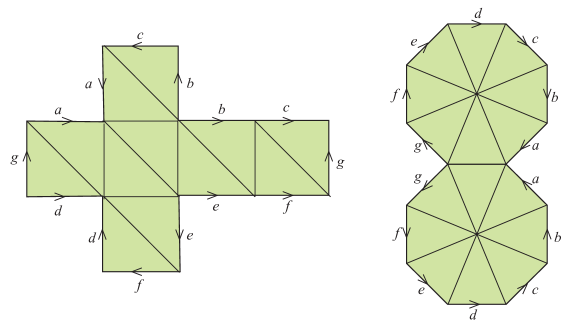
Figure 2. Two geometric $S^{2}_{(4/3,4/3,4/3,4/3,4/3,4/3,4/3,4/3)}$.

2.3. Values of the Euler characteristic

The next result proves that if a 2-conemanifold has some geometric structures, all of them are modeled on the same $X$ geometry.

Let $(\Sigma,P,v)$ be a 2-conemanifold having a $X$-geometry. It follows from the Gauss-Bonet that

$$\int_{\Sigma}kd\sigma+\underset{i=1}{\overset{k}{\sum}}(2\pi-\frac{2\pi}{r_{i}})=2\pi\chi(\Sigma)$$

where $k$, Gauss curvature, is $-1,0,1$ if $X$ is equal to $H^{2}$, $E^{2}$ or $S^{2}$, respectively. This is equivalent to

$$\int_{\Sigma}kd\sigma=2\pi(\chi(\Sigma)+\underset{i=1}{\overset{k}{\sum}}(\frac{1}{r_{i}}-1))=2\pi\chi^{c}(\Sigma)$$

Proposition 2.1.

Let $(\Sigma,P,v)$ be a 2-conemanifold having a $X$-geometry. Then $\chi^{c}(\Sigma)$ is $<0$, $=0$ or $>0$ when $X$ is equal to $H^{2}$, $E^{2}$ or $S^{2}$ respectively. ∎

2.4. The 2-conemanifolds $(O,0|2,3,r)$

Consider the 2-conemanifold $(\Sigma,P,v)=(O,0|2,3,r)$, the 2-sphere with three singular points and valuation $v(x_{1})=2$, $v(x_{2})=3$, and $v(x_{3})=r$. This notation is suggested by the Seifert notation in [6].

(2.1) $$\chi^{c}((O,0|2,3,r))=2-3+\frac{1}{2}+\frac{1}{3}+\frac{1}{r}=-\frac{1}{6}+\frac{1}{r}$$

Proposition 2.2.

The 2-conemanifold $(O,0|2,3,r)$ has Euclidean geometry for $r=6$; spherical geometry for $\frac{6}{5}<r<6$; and hyperbolic geometry for $r>6$.

Proof.

By (2.1)

(2.2) $$\chi^{c}((O,0|2,3,r))\left\{\begin{array}[]{c}<\\ =\\ >\end{array}\right\}0\Leftrightarrow r\left\{\begin{array}[]{c}>\\ =\\ <\end{array}\right\}6$$

Therefore, Proposition 2.1 indicates which type of geometry we should look for.

The hyperbolic metric in the Poincaré disc model, the open unit disc

$$D_{1}=\left\{z=x+iy\;|\;x^{2}+y^{2}<1\right\}$$

is given by

$$ds^{2}=\frac{4dzd\overline{z}}{(1-z\overline{z})^{2}}.$$

In order to apply degeneration on geometric structures is more convenient to work with a disc in $\mathbb{C}$ with radius $\frac{1}{\sqrt{S}}$. Then the dilatation

$$\begin{array}[]{cccc}\lambda:&D_{\frac{1}{\sqrt{S}}}&\longrightarrow&D_{1}\\ &z&\to&\sqrt{S}z\end{array}$$

is an isometry if and only if the metric on $D_{\frac{1}{\sqrt{S}}}$ is given by

$$ds^{2}=\frac{4Sdzd\overline{z}}{(1-Sz\overline{z})^{2}},\quad 1\geq S>0$$

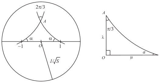
Figure 3. The hyperbolic plane and a hyperbolic triangle.

Figure 3 shows a hyperbolic triangle $T$ . The angles at the two vertices placed at the points $(-1,0)$ and $(1,0)$ are both $\alpha$. The remaining vertex has an angle of $2\pi/3$. Lets us relate the angle $\alpha$ with $S$ using well known formulas for hyperbolic triangles.

$$\cosh\mu=\frac{\cos\frac{\pi}{3}}{\sin\alpha}=\frac{1}{2\sin\alpha};\qquad\cosh\lambda=\frac{\cos\alpha}{\sin\frac{\pi}{3}}=\frac{2\cos\alpha}{\sqrt{3}}$$

$$\mu = \int_{0}^{1}\sqrt{\frac{4S}{(1-St^{2})^{2}}}dt=\int_{0}^{1}\frac{2\sqrt{S}}{(1-St^{2})}dt=$$

$$= \lg(1+\sqrt{S}t)-\lg(1-\sqrt{S}t)|_{0}^{1}=\lg\frac{1+\sqrt{S}}{1-\sqrt{S}}$$

$$\Rightarrow\quad e^{\mu}=\frac{1+\sqrt{S}}{1-\sqrt{S}}\quad\Rightarrow\quad\cosh\mu=\frac{e^{2\mu}+1}{2e^{\mu}}=\frac{1+S}{1-S}$$

Therefore

(2.3) $$\frac{1}{2\sin\alpha}=\frac{1+S}{1-S}\quad\Rightarrow\boxed{S=\frac{1-2\sin\alpha}{1+2\sin\alpha}}$$

Analogously, $\mathbb{C}P^{1}$ with the spherical Riemannian metric,

$$ds^{2}=\frac{-4Sdzd\overline{z}}{(1-Sz\overline{z})^{2}},\quad S<0$$

is the stereographic projection of the sphere $S^{2}$ with radius $\frac{1}{\sqrt{-S}}$ endowed with a Riemannian metric isometric to the usual spherical metric on the unit sphere in $\mathbb{R}^{3}$. The circle of radius $\frac{1}{\sqrt{-S}}$ is the equator. Figure 4 shows the spherical triangle $T$ analogous to the hyperbolic case.

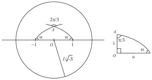
Figure 4. The spherical case.

In this spherical case

$$\cos\mu=\frac{\cos\frac{\pi}{3}}{\sin\alpha}=\frac{1}{2\sin\alpha}$$

$$\mu=\int_{0}^{1}\sqrt{\frac{-4S}{(1-St^{2})^{2}}}dt=\int_{0}^{1}\frac{i2\sqrt{S}}{(1-St^{2})}dt$$

$$\Rightarrow-i\mu=\lg(1+\sqrt{S}t)-\lg(1-\sqrt{S}t)|_{0}^{1}=\lg\frac{1+\sqrt{S}}{1-\sqrt{S}}$$

$$\Rightarrow\quad e^{-i\mu}=\frac{1+\sqrt{S}}{1-\sqrt{S}}\quad\Rightarrow\quad\cos\mu=\frac{e^{i\mu}+e^{-i\mu}}{2}=\frac{1+S}{1-S}$$

Therefore as before

(2.4) $$\frac{1}{2\sin\alpha}=\frac{1+S}{1-S}\quad\Rightarrow\boxed{S=\frac{1-2\sin\alpha}{1+2\sin\alpha}}$$

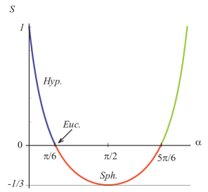
Figure 5. The graphic $S(\alpha)$.

Figure 5 shows the graph of $S$ as a function of $\alpha$ and the values where the triangle $T$ exists in hyperbolic plane (Hyp.), Euclidian plane (Euc.) and sphere (Sph.). Therefore

$$\alpha=0\quad\Leftrightarrow\quad S=1;\qquad\alpha=\frac{\pi}{6}\quad\Leftrightarrow\quad S=0.$$

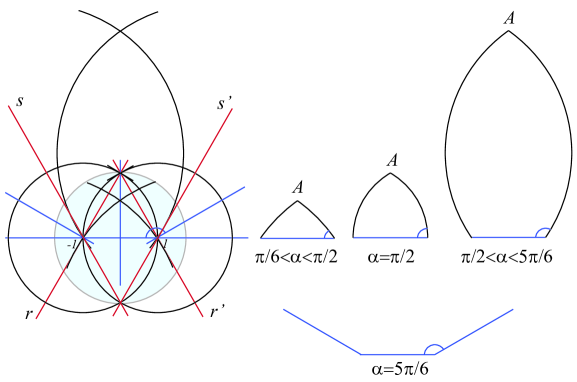
Figure 6. Some spherical triangles and the limit case.

The case $S=0$ correspond to the disc of infinite radius: the Euclidian case. The hyperbolic triangle $T$ exists for $0<\alpha<\frac{\pi}{6}$; for $\alpha=\frac{\pi}{6}$ is an Euclidean triangle and for $\frac{\pi}{6}<\alpha<\frac{5\pi}{6}$ is a spherical triangle.

Figure 6 shows some cases in the stereographic projection of the sphere $S^{2}$ of radius $\frac{1}{\sqrt{-S}}$ in the plane, where the shadowed disc corresponds to one of the hemispheres of $S^{2}$ limited by the equator (in the figure $S=-\frac{1}{3}$). The edge between the two angles $\alpha$ is common to all the triangles, and it is the segment lying between points $(-1,0)$ and $(1,0)$. The other two edges are part of circles centered at point in the lines $r$ and $r^{\prime}$, for $\frac{\pi}{6}<\alpha\leq\frac{\pi}{2}$, and in the lines $s$ and $s^{\prime}$ for $\frac{\pi}{2}\leq\alpha\leq\frac{5\pi}{6}$. The radius of this circles is a function of $S$. In the same figure are depicted three triangles, and also the limit case $S=0,\,\alpha=\frac{5\pi}{6}$ where the geometry becomes Euclidean.

The geometric 2-conemanifold $(O,0|2,3,r)$, where $r=\frac{\pi}{\alpha}$, is obtained as the quotient of $T$ by identifying the two edges, meeting in $A$, by a $(2\pi/3)$-rotation isometry centered at $A$ and identifying the two halfs of the other edge by a $\pi$-rotation isometry centered at $O$. ∎

2.5. The holonomy

Let $(\Sigma,P,v)$ be a 2-conemanifold having an $X$-geometry. The holonomy map of $(\Sigma,P,v)$ is a homomorphism

$$\omega:\pi_{1}(\Sigma\setminus P)\longrightarrow I\!so(X)$$

defined as follows.

Let $\gamma$ be a meridian of $x\in P$. Develop $\Sigma$ over $X$ along $\gamma$; the isometry relating the two ends of this developing is, by definition, $\omega(\gamma)$.

The image of $\omega$ is called the holonomy of $(\Sigma,P,v)$.

Thurston ([8], [3]) proved that if the valuations are all natural numbers, the conemanifold is an orbifold obtained as the quotient of $X$ by the holonomy.

Proposition 2.3.

Consider the 2-conemanifold $(O,0|2,3,r)$ with its corresponding $X$-geometry. Let $\rho$ denote the rotation of angle $\frac{2\pi}{r}$around the point $0$. Let $\tau_{\pm}$ denote the translation sending $0$ to $\pm 1$ in the model of radius $\frac{1}{\sqrt{|S|}}$. This translation will be hyperbolic, Euclidean or spherical, according to $X$. Then the image of the holonomy of the $X$-geometry of $(O,0|2,3,r)$ is the subgroup of $Iso^{+}X$ generated by the rotations $a$ and $b$, conjugate to $\rho$ by $\tau_{\pm}$.

Proof.

The fundamental group $\pi_{1}(\Sigma\setminus P)$ is the fundamental group of a sphere with three punctures.

$$\pi_{1}(\Sigma\setminus P)=|c,d:-|$$

where $c,d$ are meridians of the conic points with valuation $3$ and $2$ respectively.

The holonomy map is, by definition, a homomorphism

(2.5) $$\begin{array}[]{cccc}\omega:&\pi_{1}(\Sigma\setminus P)&\longrightarrow&I\!so(X)\\ &c&\rightarrow&\omega(c)\\ &d&\rightarrow&\omega(d)\end{array}$$

where $(\omega(c))^{3}=I\!dentity$ and $(\omega(d))^{2}=I\!dentity$. Therefore the holonomy map $\omega$ factors through the group

$$|c,d:c^{3}=d^{2}=1|$$

We change the above presentation using $a=dc^{-1}$ and $b=ccd^{-1}$. Then $d=ac$ and $c=ba,\quad\Rightarrow d=aba$.

$$|c,d:c^{3}=d^{2}=1|=|a,b:(ba)^{3}=(aba)^{2}=1|$$

On the other hand $a$ and $b$ are conjugate: $d^{-1}bd=d^{-1}cc=dc^{-1}=a$. Therefore $\omega(a)$ is the rotation of angle $\frac{2\pi}{r}$ around the point $1\in D_{S}$, and $\omega(b)$ is its conjugate by the rotation of $\pi$ around the point $0\in D_{S}$, or equivalently, $\omega(b)$ is the rotation of angle $\frac{2\pi}{r}$ around the point $-1\in D_{S}$. ∎

3. Some 3-dimensional holonomies

The geometry $(X_{(S,S)},Q)$, is a particular case of the geometry $(X_{(R,S)},Q)$ studied in [2]. We recall this particular geometry in the following subsection. In the remain of the section we will lift the holonomies of $(O,0|2,3,r)$, constructed in the above section, to the group of isometries of $(X_{(S,S)},Q)$.

3.1. The Riemanian geometry $(X_{(S,S)},Q)$

The matrix product on the following set of $2\times 2$ complex matrices

$$X_{(S,S)}=\left\{\left[\begin{array}[]{cc}t-iSz&\sqrt{S}(x+iy)\\ \sqrt{S}(x-iy)&t+iSz\end{array}\right]\,\left|\,x,y,z,t\in\mathbb{R},t^{2}+S^{2}z^{2}-S(x^{2}+y^{2})=1\right.\right\}$$

provides a Lie group structure on the 3-dimensional quadric

$$X_{(S,S)}=\left\{(x,y,z.t)\in\mathbb{R}^{4}\,|\,t^{2}+S^{2}z^{2}-S(x^{2}+y^{2})=1\right\}$$

contained in $\mathbb{R}^{4}$.

It is proved in [2] that $X_{(S,S)}$ is isomorphic to the 3-sphere if $S<0$ and it is isomorphic to $SL(2,\mathbb{R})$ if $S>0$. The limit Lie group when $S\rightarrow 0$

$$X_{1}=\lim_{S\rightarrow 0}X_{(S,S)}$$

is isomorphic to the Heisenberg group.

The metric $Q$ in $X_{(S,S)}$ is the left invariant metric defined, in the canonical basis $e_{1}=(1,0,0,1),e_{2}=(0,1,0,1),e_{3}=(0,0,1,1)$ at the identity $(0,0,0,1)$, by the identity matrix $<1,1,1,1>$. Observe that $(X_{-1,-1},Q)$ is the spherical geometry $S^{3}$, $(X_{1,1},Q)$ is the $\widetilde{SL(2,\mathbb{R})}$ geometry and $(X_{1},Q)$ is a Nil geometry. Therefore, in this way we can study continuos transitions between some of the Thurston’s geometries. Namely, Spherical-Nil-$\widetilde{SL(2,\mathbb{R})}$.

Each element $q\in X_{(S,S)}$ defines an isometry $l_{q}$ by left product. The right product $r_{q^{\prime}}$ by any diagonal element $q^{\prime}$ of $X_{(S,S)}$ is also an isometry. The left-right notation for an isometry is a pair of elements of $X_{(S,S)}$ $(q,q^{\prime})$, where $q$ acts by left product and $q^{\prime}$ acts by right product. The composition of such isometries is given by

$$(q_{1},q_{1}^{\prime})\cdot(q_{2},q_{2}^{\prime})=(q_{2}q_{1},q_{1}^{\prime}q_{2}^{\prime})$$

These isometries can be expressed also as the restriction to $X_{(S,S)}$ of linear maps in $\mathbb{R}^{4}$ and we denote by $lm(q)$ and $rm(q^{\prime})$ the corresponding $4\times 4$ matrices. This second notation is convenient when we consider the limit situation $S\rightarrow 0$.

The manifold $X_{(S,S)}$ has a Seifert fibered structure, where the $\mathbb{S}^{1}$-action is given by the right product

$$\begin{array}[]{ccc}X(S,S)\times\mathbb{S}^{1}&\longrightarrow&X(S,S)\\ \begin{bmatrix}\ast&\sqrt{R}(x+iy)\\ \ast&t+iSz\end{bmatrix}\begin{bmatrix}e^{-i\theta}&0\\ 0&e^{i\theta}\end{bmatrix}&\rightarrow&\begin{bmatrix}\ast&e^{i\theta}\left(\sqrt{R}(x+iy)\right)\\ \ast&e^{i\theta}\left(t+iSz\right)\end{bmatrix},\end{array}$$

Its base space $D_{S}$ is $\mathbb{C}P^{1}$ for $S<0$, and $D_{S}=\left\{w\in\mathbb{C}P^{1};w\overline{w}<\frac{1}{S}\right\}$ for $S>0$. The projection of the Seifert fibered structure $X_{(S,S)}$ is given by

$$\begin{array}[]{ccc}p:X_{(S,S)}&\longrightarrow&D_{S}\\ (x,y,z,t)&\rightarrow&\frac{x+iy}{t+iSz}\end{array}.$$

The action of $l_{q}$ on $X_{(S,S)}$, where $q=\left[\begin{array}[]{cc}d-iSc&\sqrt{S}(a+ib)\\ \sqrt{S}(a-ib)&d+iSc\end{array}\right]$, projects onto the homography

$$\begin{array}[]{ccc}h_{q}:D_{S}&\longrightarrow&D_{S}\\ w&\rightarrow&\frac{(d-iSc)w+(a+bi)}{S(a-bi)w+(d+iSc)}\end{array}$$

of $D_{S}$.

For our purposes it is convenient to write the metric matrix $Q$ of $X_{(S,S)}$ in Seifert product coordinates $(\mu,\nu,\zeta)\in D_{S}\times\mathbb{S}^{1}$. The metric matrix of $Q$ in these coordinates is the following:

(3.1) $$Q((\mu,\nu,\theta)=\left[\begin{array}[]{ccc}\frac{\nu^{2}+1}{\left(1-S\left(\mu^{2}+\nu^{2}\right)\right)^{2}}&-\frac{\mu\nu}{\left(1-S\left(\mu^{2}+\nu^{2}\right)\right)^{2}}&\frac{\nu}{S\left(1-S\left(\mu^{2}+\nu^{2}\right)\right)}\\ &&\\ \ast&\frac{\mu^{2}+1}{\left(1-S\left(\mu^{2}+\nu^{2}\right)\right)^{2}}&-\frac{\mu}{S\left(1-S\left(\mu^{2}+\nu^{2}\right)\right)}\\ &&\\ \ast&\ast&\frac{1}{S^{2}}\end{array}\right].$$

Note that this formula makes sense for all $X_{(S,S)}$ for $S>0$. For $S<0$ it applies only out of the 1-sphere $C_{\infty}=\left\{(x,y,0,0)\in X_{(S,S)}|-S(x^{2}+y^{2})=1\right\}$.

Observe that in these coordinates the value of $Q$ do not depend on the third coordinate $\zeta$, it only depends on the coordinates in the base of the Seifert fibration. It is a fibred metric.

It is an easy exercise to check that the $2\times 2$ principal submatrix of (3.1), which is the restriction to the base of the Seifert manifold $X_{(-1,1)}$, coincides with the hyperbolic metric on the upper sheet $UH$ of the hyperboloid $-x_{1}^{2}-x_{2}^{2}+x_{3}^{2}=1/S$ for $S>0$, and with the usual metric on the 2-sphere $\mathbb{S}_{1/\sqrt{|S|}}^{2}$ of radius $1/\sqrt{|S|}$ for $S<0$. Indeed, in case $S>0$, it is enough to consider the pullback of the usual metric in $UH$ by the map:

$$\begin{array}[]{cccc}\pi_{UH}:&\mathbb{R}^{2}&\longrightarrow&UH=\left\{(x_{1},x_{2},x_{3})\in\mathbb{R}^{3}|-x_{1}^{2}-x_{2}^{2}+x_{3}^{2}=1/S,x_{3}>0\right\}\\ &(\mu,\nu)&\rightarrow&\left(\frac{\mu}{\sqrt{1-S(\mu^{2}+\nu^{2})}},\frac{\nu}{\sqrt{1-S(\mu^{2}+\nu^{2})}},\frac{1}{\sqrt{S(1-S(\mu^{2}+\nu^{2}))}}\right)\end{array}$$

In case $S<0$, consider the pullback of the usual metric in the north hemisphere $\mathbb{S}_{+}^{2}$ of $\mathbb{S}_{1/\sqrt{|S|}}^{2}$ (induced by the Euclidean metric in $\mathbb{R}^{3}$) by the map:

$$\begin{array}[]{cccc}\pi_{\mathbb{S}_{+}^{2}}:&\mathbb{R}^{2}&\longrightarrow&\mathbb{S}_{+}^{2}=\left\{(x_{1},x_{2},x_{3})\in\mathbb{R}^{3}|x_{1}^{2}+x_{2}^{2}+x_{3}^{2}=1/|S|,x_{3}>0\right\}\\ &(\mu,\nu)&\rightarrow&\left(\frac{\mu}{\sqrt{1-(|S|(\mu^{2}+\nu^{2}))}},\frac{\nu}{\sqrt{1-(|S|(\mu^{2}+\nu^{2}))}},\frac{1}{\sqrt{|S|(1-|S|(\mu^{2}+\nu^{2}))}}\right)\end{array}$$

These maps are the projections from the origen $(0,0,0)$ of the tangent plane at $(0,0,1/S)$ to $UH$ (or $\mathbb{S}_{+}^{2}$, as the case may be). Their inverse maps define the Klein-Beltrami models of the hyperbolic and spherical 2-dimensional geometries, respectively (see Figure 7). Therefore the metric on the base of the Seifert structure of $X_{(S,S)}$, in coordinates $(\mu,\nu)\in D_{S}$, is the usual one of the hyperbolic geometry for $S>0$, and of the spherical geometry for $S<0$.

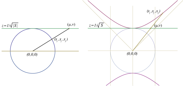
Figure 7. The projections $\pi_{NH}$ and $\pi_{UH}$.

3.2. Lifting holonomies

In this section we find the subgroups of isometries of $(X_{(S,S)},Q)$ that project onto the holonomies of $(O,0|2,3,r)$ under the projection

$$p:X_{(S,S)}\longrightarrow D_{S}.$$

In a different section we will realize this lifted holonomies by constructing suitable $3$-conemanifolds modelled on $(X_{(S,S)},Q)$.

We first define two isometries in $(X_{(S,S)},Q)$, $S\neq 0$, that projet onto the elements $a$ and $b$, defined in Proposition 2.3, under the map

$$p:X_{(S,S)}\longrightarrow D_{S}$$

as follows.

Consider the isometry $R(\alpha,\theta)$ of $(X_{(S,S)},Q)$, given in left-right notation by

(3.2) $$R(\alpha,\theta)=\left(\left[\begin{array}[]{cc}e^{i\alpha}&0\\ 0&e^{-i\alpha}\end{array}\right],\left[\begin{array}[]{cc}e^{-i\theta}&0\\ 0&e^{i\theta}\end{array}\right]\right)\quad\overset{p}{\longrightarrow}\quad w=e^{2i\alpha}z.$$

As a linear map it is given by the following matrix

(3.3) $$lm(R(\alpha,\theta))=\left[\begin{array}[]{cc}\begin{array}[]{cc}\cos(\alpha+\theta)&-\sin(\alpha+\theta)\\ \sin(\alpha+\theta)&\cos(\alpha+\theta)\end{array}&0\\ 0&\begin{array}[]{cc}\cos(\alpha-\theta)&\frac{-\sin(\alpha-\theta)}{S}\\ S\sin(\alpha-\theta)&\cos(\alpha-\theta)\end{array}\end{array}\right]$$

The projection $p:X_{(S,S)}\longrightarrow D_{S}$ maps this isometry $R(\alpha,\theta)$ onto a rotation of angle $2\alpha$ around the origin $O\in D_{S}$.

The translations in $X_{(S,S)}$ sending the point $(0,0,0,1)$, (such that $p(0,0,0,1)=0\in D_{S}$), to the point $\frac{1}{\sqrt{|1-S|}}(\pm 1,0,0,1)$ (such that $p(\frac{1}{\sqrt{|1-S|}}(\pm 1,0,0,1))=\pm 1\in D_{S}$) are respectively

(3.4) $$\begin{array}[]{llll}t_{1}&=\left(\frac{1}{\sqrt{|1-S|}}\left[\begin{array}[]{cc}1&\sqrt{S}\\ \sqrt{S}&1\end{array}\right],\left[\begin{array}[]{cc}1&0\\ 0&1\end{array}\right]\right)&\overset{p}{\longrightarrow}&w=\frac{z+1}{Sz+1}\\ t_{-1}&=\left(\frac{1}{\sqrt{|1-S|}}\left[\begin{array}[]{cc}1&-\sqrt{S}\\ -\sqrt{S}&1\end{array}\right],\left[\begin{array}[]{cc}1&0\\ 0&1\end{array}\right]\right)&\overset{p}{\longrightarrow}&w=\frac{z-1}{-Sz+1}\end{array}.$$

In linear matrix notation they are

(3.9) $$lm(t_{1}) = \frac{1}{\sqrt{|1-S|}}\left[\begin{array}[]{cccc}1&0&0&1\\ 0&1&S&0\\ 0&1&1&0\\ S&0&0&1\end{array}\right];$$

(3.14) $$lm(t_{-1}) = \frac{1}{\sqrt{|1-S|}}\left[\begin{array}[]{cccc}1&0&0&-1\\ 0&1&-S&0\\ 0&-1&1&0\\ -S&0&0&1\end{array}\right].$$

Define $a(\alpha,\theta)$ and $b(\alpha,\theta)$ as the conjugate elements of $R(\alpha,\theta)$ by the translations $t_{1}$ and $t_{-1}$ respectively. Then the projections by $p$ of $a(\alpha,\theta)$ and $b(\alpha,\theta)$ coincide, respectively, with the elements $a$ and $b$ defined in Proposition 2.3, where $\alpha=\pi/r$.

(3.15) $$a(\alpha,\theta) = t_{1}\cdot R(\alpha,\theta)\cdot t_{1}^{-1}$$

(3.16) $$b(\alpha,\theta) = t_{-1}\cdot R(\alpha,\theta)\cdot t_{-1}^{-1}$$

After some computations and substitution of the value of $S$ as a function of $\alpha$, by means of equations (2.4) and (2.3), the expressions for $a(\alpha,\theta)$ and $b(\alpha,\theta)$ in left-right notation become

$$a(\alpha,\theta) = (M,R)$$

$$b(\alpha,\theta) = (N,R)$$

where

$$M = \frac{1}{2}\left[\begin{array}[]{cc}2\cos(\alpha)+i&-i\sqrt{2\cos(2\alpha)-1}\\ i\sqrt{2\cos(2\alpha)-1}&2\cos(\alpha)-i\end{array}\right]$$

$$N = \frac{1}{2}\left[\begin{array}[]{cc}2\cos(\alpha)+i&i\sqrt{2\cos(2\alpha)-1}\\ -i\sqrt{2\cos(2\alpha)-1}&2\cos(\alpha)-i\end{array}\right]$$

$$R = \left[\begin{array}[]{cc}e^{-i\theta}&0\\ 0&e^{i\theta}\end{array}\right]$$

and as $4\times 4$ matrices they are

(3.20) $$lm(a(\alpha,\theta))=\frac{1}{2}\left[\begin{array}[]{cc}A_{11}&A_{12}\\ A_{21}&A_{22}\end{array}\right]$$

and

(3.21) $$lm(b(\alpha,\theta))=\frac{1}{2}\left[\begin{array}[]{cc}A_{11}&-A_{12}\\ -A_{21}&A_{22}\end{array}\right],$$

where

$$A_{11} = \left(\begin{array}[]{cc}2\cos(\alpha)\cos(\theta)-\sin(\theta)&-2\cos(\alpha)\sin(\theta)-\cos(\theta)\\ 2\cos(\alpha)\sin(\theta)+\cos(\theta)&2\cos(\alpha)\cos(\theta)-\sin(\theta)\end{array}\right)$$

$$A_{12} = \left(\begin{array}[]{cc}(1-2\sin(\alpha))\cos(\theta)&(1+2\sin(\alpha))\sin(\theta)\\ (1-2\sin(\alpha)\sin(\theta)&-(1+2\sin(\alpha))\cos(\theta)\end{array}\right)$$

$$A_{21} = \left(\begin{array}[]{cc}(1+2\sin(\alpha))\cos(\theta)&-(1+2\sin(\alpha))\sin(\theta)\\ -(1-2\sin(\alpha))\sin(\theta)&-(1-2\sin(\alpha))\cos(\theta)\end{array}\right)$$

$$A_{22} = \left(\begin{array}[]{cc}2\cos(\alpha)\cos(\theta)+\sin(\theta)&\frac{(1+2\sin(\alpha))(2\cos(\alpha)\sin(\theta)-\cos(\theta))}{1-2\sin(\alpha)}\\ \frac{(1-2\sin(\alpha))(-2\cos(\alpha)\sin(\theta)+\cos(\theta))}{1+2\sin(\alpha)}&2\cos(\alpha)\cos(\theta)+\sin(\theta)\end{array}\right).$$

The two elements $a(\alpha,\theta)$ and $b(\alpha,\theta)$ are the generators, for each $\theta$, of a group of isometries of $X_{(S,S)}$, $S\neq 0$, that projects onto the holonomy of the conemanifold $(O,0|2,3,r)$, where $\alpha=\frac{\pi}{r}$.

The case $S=0$ is a limit case. By equations (2.4) and (2.3)

$$S=0\Longleftrightarrow\alpha=\frac{\pi}{6}$$

The natural definition is

(3.26) $$lm(a(\frac{\pi}{6},\theta)) =\lim_{\alpha\to\frac{\pi}{6}}lm(a(\alpha,\theta))$$

(3.27) $$lm(b(\frac{\pi}{6},\theta)) =\lim_{\alpha\to\frac{\pi}{6}}lm(b(\alpha,\theta))$$

The values of all the elements in these matrices are finite but the value of the element $(1,2)$ in $A_{22}$ for $\alpha=\pi/6$, which is

(3.28) $$\lim_{\alpha\rightarrow\frac{\pi}{6}}\frac{-(1+2\sin(\alpha))(-2\cos(\alpha)\sin(\theta)+\cos(\theta))}{1-2\sin(\alpha)}\\ =\frac{-2(-\sqrt{3}\sin(\theta)+\cos(\theta))}{0},$$

becomes infinite or indeterminate according to the value of $\theta$. On the other hand the value of the element $(2,2)$ in $A_{2,2}$ which is

$$\sqrt{3}\cos(\theta)+\sin(\theta)$$

should be equal to $1$ in order that $a(\frac{\pi}{6},\theta)$ and $b(\frac{\pi}{6},\theta)$ be isometries of the group $X_{1}$. Therefore

$$\sqrt{3}\cos(\theta)+\sin(\theta)=1\Longleftrightarrow\theta=\frac{\pi}{6}$$

for this value of $\theta$ the element (3.28) is indeterminate and can be obtained by the l’Hopital rule.

Observe that if $\theta=\alpha+t(6\alpha-\pi)$, $t\in\mathbb{R}$, then

$$\alpha\to\frac{\pi}{6}\quad\Longrightarrow\quad\theta\to\frac{\pi}{6}$$

Lets define

(3.33) $$a_{t}= \lim_{\alpha\to\frac{\pi}{6}}lm(a(\alpha,\alpha+t(6\alpha-\pi)))=\left[\begin{array}[]{cccc}\frac{1}{2}&-\frac{\sqrt{3}}{2}&0&\frac{1}{2}\\ \frac{\sqrt{3}}{2}&\frac{1}{2}&0&-\frac{\sqrt{3}}{2}\\ \frac{\sqrt{3}}{2}&-\frac{1}{2}&1&-\frac{1}{2}\sqrt{3}(8t+1)\\ 0&0&0&1\end{array}\right]$$

(3.39) $$b_{t}= \lim_{\alpha\to\frac{\pi}{6}}lm(b(\alpha,\alpha+t(6\alpha-\pi)))=\left[\begin{array}[]{cccc}\frac{1}{2}&-\frac{\sqrt{3}}{2}&0&-\frac{1}{2}\\ \frac{\sqrt{3}}{2}&\frac{1}{2}&0&\frac{\sqrt{3}}{2}\\ -\frac{\sqrt{3}}{2}&\frac{1}{2}&1&-\frac{1}{2}\sqrt{3}(8t+1)\\ 0&0&0&1\end{array}\right]$$

For each $t\in\mathbb{R}$, $a_{t}$ and $b_{t}$ are the generators of a subgroup of isometries in $X_{1}$ which projets on the holonomy of the conemanifold $(O0|2,3,6)$.

3.3. Representations of the trefoil knot group

Proposition 3.1.

Let $\mathbb{T}$ be the oriented left-handed trefoil knot in $\mathbb{S}^{3}$ (Figure 8), with group

$$G(\mathbb{T})=\pi_{1}(\mathbb{S}^{3}\setminus K)=|a,b;aba=bab|$$

where $a$ and $b$ are meridian elements. The maps

(3.40) $$\begin{array}[]{cccc}\omega_{\mathbb{T}}:&G(\mathbb{T})=\pi_{1}(\mathbb{S}^{3}\setminus\mathbb{T})&\longrightarrow&Isom(X_{(S,S)},Q),\quad S\neq 0\\ &a&\to&a(\alpha,\theta)\\ &b&\to&b(\alpha,\theta)\end{array}$$

and

(3.41) $$\begin{array}[]{cccc}\omega_{\mathbb{T}}:&G(\mathbb{T})=\pi_{1}(\mathbb{S}^{3}\setminus\mathbb{T})&\longrightarrow&Isom(X_{1},Q)\\ &a&\to&a_{t}\\ &b&\to&b_{t}\end{array}$$

are homomorphisms.

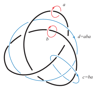
Figure 8. The trefoil knot.

Proof.

To prove that the map $\omega_{\mathbb{T}}$ in (3.40) is a homomorphism it is enough to check the relator

(3.42) $$a(\alpha,\theta)b(\alpha,\theta)a(\alpha,\theta)=b(\alpha,\theta)a(\alpha,\theta)b(\alpha,\theta)$$

or equivalently

(3.43) $$(MNM,R^{3})=(NMN,R^{3})$$

A straightforward computation yields

$$(NM)^{3}=(MNM)^{2}=-I_{2\times 2}$$

Therefore

$$MNMNMN=MNMMNM=-I_{2\times 2}\Longrightarrow NMN=MNM=\left[\begin{array}[]{cc}i&0\\ 0&-i\end{array}\right]$$

The proof that the same is true in (3.41)

$$a_{t}b_{t}a_{t}=b_{t}a_{t}b_{t}$$

can be done by direct computation using (3.33). In fact

$$a_{t}b_{t}a_{t}=b_{t}a_{t}b_{t}=\left[\begin{array}[]{cccc}-1&0&0&0\\ 0&-1&0&0\\ 0&0&1&-2\sqrt{3}(6t+1)\\ 0&0&0&1\end{array}\right]$$

∎

Corollary 3.1.

For each pair $(\alpha,\theta)$, $\alpha\in\left[0,\frac{\pi}{6}\right)\cup\left(\frac{\pi}{6},\frac{5\pi}{6}\right)$, there exits a group of isometries in $(X_{(S,S)},Q)$ generated by $a(\alpha,\theta)$ and $b(\alpha,\theta)$, which is the epimorphic image of the trefoil knot group, such that it projects by $p:X_{(S,S)}\longrightarrow D_{S}$, onto the holonomy of $(O,0|2,3,r)$, $r=\frac{\pi}{\alpha}$.

For $\alpha=\frac{\pi}{6}$ there exists infinite pairs of isometries $(a_{t},b_{t})$, $t\in\mathbb{R}$, of $(X_{1},Q)$ generating subgroups which are the epimorphic image of the trefoil knot group, such that they all projects by $p:X_{1}\longrightarrow\mathbb{C}$, onto the holonomy of $(O,0|2,3,6)$. ∎

Summary 1.

The holonomy (2.5) of the geometric structure of the 2-conemanifold $(O,0|2,3,r)$ is generated by $\omega(c)$ and $\omega(d)$, where $c=ba$, $d=aba$ and

$$\pi_{1}((O0|2,3,r))=|c,d;-|.$$

For each $r=\frac{\pi}{\alpha}$, $0\leq\alpha<\frac{5\pi}{6}$, $\alpha\neq\frac{\pi}{6}$, the 2 conemanifold $(O,0|2,3,r)$ has a geometric structure modeled in the disc $D_{S}$ of radius $1/\sqrt{|S|}$, where $S=\frac{1-2\sin\alpha}{1+2\sin\alpha}$. For $\alpha=\frac{\pi}{6}$, $D_{S}$ is $\mathbb{C}$ and the geometry is Euclidean.

For each pair $(\alpha,\theta)$, $\alpha\in\left[0,\frac{\pi}{6}\right)\cup\left(\frac{\pi}{6},\frac{5\pi}{6}\right)$, there exits a group of isometries in $(X_{(S,S)},Q)$ generated by $a(\alpha,\theta)$ and $b(\alpha,\theta)$, which is the epimorphic image of the trefoil knot group, such that it projects by $p:X_{(S,S)}\longrightarrow D_{S}$, onto the holonomy of $(O,0|2,3,r)$, $r=\frac{\pi}{\alpha}$.

For $\alpha=\frac{\pi}{6}$ there exists infinite pairs of isometries $(a_{t},b_{t})$, $t\in\mathbb{R}$, of $(X_{1},Q)$ generating subgroups which are the epimorphic image of the trefoil knot group, such that it projects by $p:X_{1}\longrightarrow\mathbb{C}$, on the holonomy of $(O,0|2,3,6)$.

4. Construction of the 3-conemanifolds with holonomy $\omega_{\mathbb{T}}(G(\mathbb{T}))$

Next we construct geometrically the 3-conemanifolds whose holonomies are the above subgroups $\omega_{\mathbb{T}}(G(\mathbb{T}))$ in (3.40) and (3.41).

Define

$$c(\alpha,\theta) = b(\alpha,\theta)\,a(\alpha,\theta)$$

$$d(\alpha,\theta) = b(\alpha,\theta)\,a(\alpha,\theta)\,b(\alpha,\theta)$$

(4.1) $$c_{t} = b_{t}\,a_{t}$$

$$d_{t} = b_{t}\,a_{t}\,b_{t}.$$

Then

(4.6) $$c(\alpha,\theta) = \left(\frac{1}{2}\left[\begin{array}[]{cc}1+2i\cos(\alpha)&\sqrt{2\cos(2\alpha)-1}\\ \sqrt{2\cos(2\alpha)-1}&1-2i\cos(\alpha)\end{array}\right],\left[\begin{array}[]{cc}e^{-2i\theta}&0\\ 0&e^{2i\theta}\end{array}\right]\right)$$

(4.11) $$d(\alpha,\theta) = \left(\left[\begin{array}[]{cc}i&0\\ 0&-i\end{array}\right],\left[\begin{array}[]{cc}e^{-3i\theta}&0\\ 0&e^{3i\theta}\end{array}\right]\right)$$

(4.16) $$c_{t} = \left[\begin{array}[]{cccc}-\frac{1}{2}&-\frac{\sqrt{3}}{2}&0&\frac{1}{2}\\ \frac{\sqrt{3}}{2}&-\frac{1}{2}&0&\frac{\sqrt{3}}{2}\\ \frac{\sqrt{3}}{2}&\frac{1}{2}&1&-\frac{1}{2}\sqrt{3}(16t+3)\\ 0&0&0&1\end{array}\right]$$

(4.21) $$d_{t} = \left[\begin{array}[]{cccc}-1&0&0&0\\ 0&-1&0&0\\ 0&0&1&-2\sqrt{3}(6t+1)\\ 0&0&0&1\end{array}\right]$$

Note that

(4.26) $$d(\alpha,\theta)d(\alpha,\theta) = \left(\left[\begin{array}[]{cc}-1&0\\ 0&-1\end{array}\right],\left[\begin{array}[]{cc}e^{-6i\theta}&0\\ 0&e^{6i\theta}\end{array}\right]\right)=$$

(4.31) $$= \left(\left[\begin{array}[]{cc}1&0\\ 0&1\end{array}\right],\left[\begin{array}[]{cc}-e^{-6i\theta}&0\\ 0&-e^{6i\theta}\end{array}\right]\right)$$

(4.37) $$d_{t}d_{t} = \left[\begin{array}[]{cccc}1&0&0&0\\ 0&1&0&0\\ 0&0&1&-4\sqrt{3}(6t+1)\\ 0&0&0&1\end{array}\right]$$

Let $(\alpha,\theta)$ be a pair such that $0\leq\alpha<\frac{\pi}{6}$. The 2-conemanifold $(O0|2,3,\pi/\alpha)$ is hyperbolic and $S>0$. Consider the hyperbolic triangle $\Delta$ in the interior of the Poincaré disc $D_{S}$ of radius $1/\sqrt{S}$, depicted in Figure 3. The inverse image of $\Delta$ by the projection $p:X_{(S,S)}\longrightarrow D_{S}$ is a fibred solid torus. Let $P=\Delta\times\mathbb{R}$ be its universal cover.

The action of

$$d(\alpha,\theta)d(\alpha,\theta)=\left(\left[\begin{array}[]{cc}1&0\\ 0&1\end{array}\right],\left[\begin{array}[]{cc}e^{-i(6\theta-\pi)}&0\\ 0&e^{i(6\theta-\pi)}\end{array}\right]\right)$$

on $X_{(S,S)}$ induces a fibre preserving action on $P$. Suppose that each fibre is oriented according to the action of $\mathbb{S}^{1}$ on $X_{(S,S)}$ (and of $\mathbb{R}$ on $P$).

The element $d(\alpha,\theta)d(\alpha,\theta)$ acts on $P$ by translation of each fibre in the positive direction by a distance of $6\theta-\pi$.

Therefore the fundamental domain $D(\alpha,\theta)$ for the action of $d(\alpha,\theta)d(\alpha,\theta)$ on $P$ is the part limited by the zero level and the $6\theta-\pi$ level. Let us study the action of $c(\alpha,\theta)$ and $d(\alpha,\theta)$ on $D(\alpha,\theta)$. Recall that this action projects onto the action of $c$ and $d$ on $\Delta$.

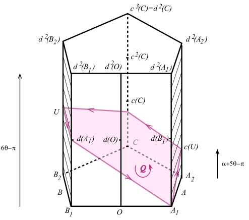
Figure 9. The fundamental domain $D(\alpha,\theta)$.

The two vertical side faces $A_{1},A_{2},d^{2}(A_{1}),d^{2}(A_{2})$ and $B_{1},B_{2},d^{2}(B_{1}),d^{2}(B_{2})$ of Figure 9 are horizontally fibred in such a way that the collapsing of these fibres yields $D(\alpha,\theta)$. The fibre $A=A_{1}A_{2}$ is sent to the fiber $U=d(\alpha,\theta)(A)$ sitting on the face lying over $B=B_{1}B_{2}$, at level $3\theta-\pi/2$. And $c(\alpha,\theta)(U)$ belongs to the face lying over $A=A_{1}A_{2}$, at level $\alpha+5\theta-\pi$:

In left-right notation

$$d(\alpha,\theta)=(NMN,R^{3})=\left(\left[\begin{array}[]{cc}i&0\\ 0&-i\end{array}\right],\left[\begin{array}[]{cc}e^{-i3\theta}&0\\ 0&e^{i3\theta}\end{array}\right]\right)=\\ =\left(\left[\begin{array}[]{cc}e^{i\pi/2}&0\\ 0&e^{-i\pi/2}\end{array}\right],\left[\begin{array}[]{cc}e^{-i3\theta}&0\\ 0&e^{i3\theta}\end{array}\right]\right)$$

and the points $A\in D_{S}$ and $B\in D_{S}$ are respectively the elements

$$A=\frac{1}{\sqrt{1-S}}\left[\begin{array}[]{cc}1&\sqrt{S}\\ \sqrt{S}&1\end{array}\right]\quad\text{and}\quad B=\frac{1}{\sqrt{1-S}}\left[\begin{array}[]{cc}1&-\sqrt{S}\\ -\sqrt{S}&1\end{array}\right].$$

Therefore, the following computation

$$U=d(\alpha,\theta)(A)=-\frac{1}{\sqrt{1-S}}\left[\begin{array}[]{cc}e^{i\pi/2}&0\\ 0&e^{-i\pi/2}\end{array}\right]\left[\begin{array}[]{cc}1&\sqrt{S}\\ \sqrt{S}&1\end{array}\right]\left[\begin{array}[]{cc}e^{-i3\theta}&0\\ 0&e^{i3\theta}\end{array}\right]\\ =\frac{1}{\sqrt{1-S}}\left[\begin{array}[]{cc}e^{-i(3\theta-\pi/2)}&\sqrt{S}e^{i(3\theta+\pi/2)}\\ \sqrt{S}e^{-i(3\theta+\pi/2)}&e^{i((3\theta-\pi/2)}\end{array}\right]\\ =\frac{1}{\sqrt{1-S}}\left[\begin{array}[]{cc}1&-\sqrt{S}\\ -\sqrt{S}&1\end{array}\right]\left[\begin{array}[]{cc}e^{-i(3\theta-\pi/2)}&0\\ 0&e^{i((3\theta-\pi/2)}\end{array}\right]\\ =B\left[\begin{array}[]{cc}e^{-i(3\theta-\pi/2)}&0\\ 0&e^{i(3\theta-\pi/2)}\end{array}\right].$$

shows that the point $U=d(\alpha,\theta)(A)$ is the point lying over the point $B$ at the $(3\theta-\pi/2)$ level. Similarly, to compute $c(\alpha,\theta)(U)$, consider the left-right notation of $c(\alpha,\theta)\circ d(\alpha,\theta)$:

$$c(\alpha,\theta)\circ d(\alpha,\theta)=(NM.NMN,R^{3}.R^{2})=(NMNMN,R^{5})$$

where

$$NMNMNM=-I_{2\times 2}\quad\Longrightarrow\\ NMNMN=-M^{-1}=-\frac{1}{1-S}\left[\begin{array}[]{cc}1&\sqrt{S}\\ \sqrt{S}&1\end{array}\right]\left[\begin{array}[]{cc}e^{i-\alpha}&0\\ 0&e^{i\alpha}\end{array}\right]\left[\begin{array}[]{cc}1&-\sqrt{S}\\ -\sqrt{S}&1\end{array}\right]$$

Then

$$c(\alpha,\theta)(U)=(c(\alpha,\theta)\circ d(\alpha,\theta))(A)=-\frac{1}{\sqrt{1-S}}M^{-1}.\left[\begin{array}[]{cc}1&\sqrt{S}\\ \sqrt{S}&1\end{array}\right].R^{5}=\\ =-\frac{1}{\sqrt{1-S}}\left[\begin{array}[]{cc}1&\sqrt{S}\\ \sqrt{S}&1\end{array}\right]\left[\begin{array}[]{cc}e^{-i\alpha}&0\\ 0&e^{i\alpha}\end{array}\right]\left[\begin{array}[]{cc}e^{-i5\theta}&0\\ 0&e^{i5\theta}\end{array}\right]=\\ =\frac{1}{\sqrt{1-S}}\left[\begin{array}[]{cc}1&\sqrt{S}\\ \sqrt{S}&1\end{array}\right]\left[\begin{array}[]{cc}e^{-i(5\theta+\alpha-\pi)}&0\\ 0&e^{i(5\theta+\alpha-\pi)}\end{array}\right]=\\ =A\left[\begin{array}[]{cc}e^{-i(5\theta+\alpha-\pi)}&0\\ 0&e^{i(5\theta+\alpha-\pi)}\end{array}\right].$$

Then, the point $c(U)$ is the point lying over $A$ at the $(5\theta+\alpha-\pi)$ level. See Figure9.

The result of the following identifications

• the two horizontal faces: ($d^{2}(A_{1}),d^{2}(A_{2}),d^{2}(C),d^{2}(B{2}),d^{2}(B_{1})$) (upper face) and ($A_{1},A_{2},C,B_{2},B_{1}$) (bottom face) by $d^{2}$;

• the two front faces ($O,A_{1},d^{2}(A_{1}),d^{2}(O)$) and ($O,B_{1},d^{2}(B_{1}),d^{2}(O)$) by $d$;

• and the two back faces ($C,A_{2},d^{2}(A_{2}),d^{2}(C)$) and ($O,B_{2},d^{2}(B_{2}),d^{2}(C)$) by $c$,

produce a Seifert manifold bounded by a torus with a foliation induced by the horizontal fibres of the side faces $A_{1},A_{2},d^{2}(A_{1}),d^{2}(A_{2})$ and $B_{1},B_{2},d^{2}(B_{1}),d^{2}(B_{2})$. Topologically this is $\mathbb{S}^{3}$ minus an open solid torus. To determine its Seifert structure consider an oriented section disc $Q$ whose orientation, followed by the orientation of the general fibre $H$, gives the positive orientation of $\mathbb{S}^{3}$. See Figure 9.

The identification of the two front faces, depicted in Figure 10 is equivalent to collapsing a curve homologous to $2Q+H$, producing a exceptional fibre of type $(2/1)$.

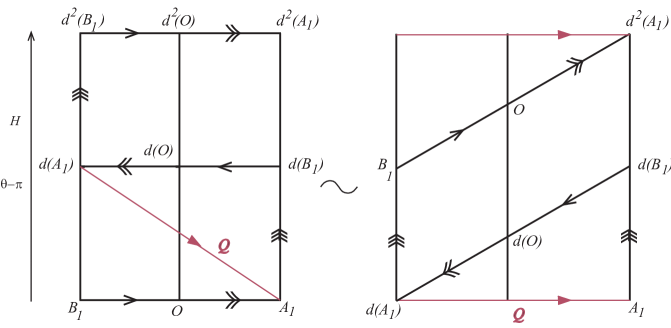
Figure 10. The two front faces in $D(\alpha,\theta)$.

The identification of the two back faces, depicted in Figure 11 is equivalent to collapsing a curve homologous to $3Q+H$, producing a exceptional fibre of type $(3/1)$.

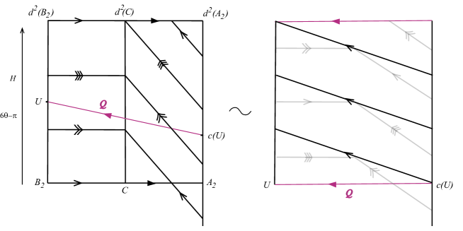
Figure 11. The two back faces in $D(\alpha,\theta)$.

Therefore the Seifert structure after the identifications in $D(\alpha,\theta)$ by $d^{2}$, $d$ and $c$ (before collapsing fibres in the torus over $A\cup B$) is

(4.38) $$(O\,o\,0|0;(2/1),(3/1))$$

minus the neighbourhood of an ordinary fibre. The fibred torus which is the boundary of the manifold after the above identifications is depicted in Figure 12. The slope of each fibre respect to the coordinates $Q$ and $H$ is $\lambda=\frac{\alpha+5\theta-\pi}{6\theta-\pi}$. If $\lambda$ is a rational number, the collapsing of the fibres in the torus is equivalent to collapsing a curve homologous to $(6\theta-\pi)Q-(\alpha+5\theta-\pi)H$.

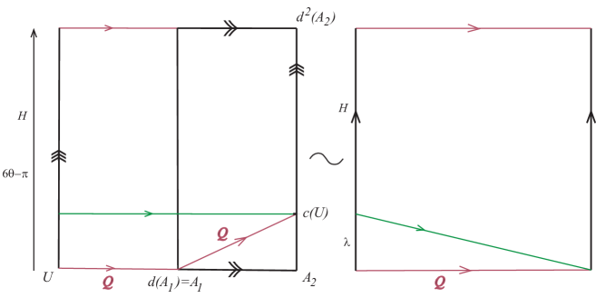
Figure 12. The torus boundy.

The resulting Seifert manifold is

$$(O\,o\,0|0;(2/1),(3/1),((6\theta-\pi)/(\alpha+5\theta-\pi))$$

$$= (O\,o\,0|-1;(2/1),(3/1),((6\theta-\pi)/(6\theta-\pi-\alpha-5\theta+\pi))$$

$$= (O\,o\,0|-1;(2/1),(3/1),((6\theta-\pi)/(\theta-\alpha))$$

This manifold is the result of $\left(\frac{6\theta-\pi}{\theta-\alpha}-6\right)$-surgery in the left-handed trefoil knot in $\mathbb{S}^{3}$. This is because the surgery is always refered to the canonical longitude and two parallel ordinary fibres in the Seifet structure $(O\,o\,0|0;(2/1),(3/1))$ in $\mathbb{S}^{3}$ are two parallel left-handed trefoil knots (can be considered in the same torus surface). Therefore, one of them is a toroidal longitude $l_{t}$ for the other, and it is easy to check (in Figure 13) that $l_{t}\,=\,l_{p}-3m\,=\,l_{c}-6m$, where $l_{p}$ is the pictorial longitude, $l_{c}$ is the canonical longitude and $m$ is the meridian of the left-handed trefoil knot.

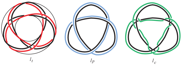
Figure 13. The toroidal, pictorial and canonical longitudes.

Theorem 4.1.

If $\frac{6\theta-\pi}{\theta-\alpha}$ is a rational number, the quotient of $P$ by the group generated by $c(\alpha,\theta)$ and $d(\alpha,\theta)$ is the Seifert manifold

$$(O\,o\,0|-1;(2/1),(3/1),((6\theta-\pi)/(\theta-\alpha))$$

which is the result of $\left(\frac{6\alpha-\pi}{\theta-\alpha}\right)$-surgery in the left-handed trefoil knot in $\mathbb{S}^{3}$. This manifold has $\widetilde{S(2,\mathbb{R})}$ geometry for $0\leq\alpha<\frac{\pi}{6}$ and spherical geometry for $\frac{\pi}{6}<\alpha<\frac{5\pi}{6}$. The conic angle $\beta$ is $2\alpha$ times the multiplicity $m$ of the exceptional fibre, where $\frac{6\alpha-\pi}{\theta-\alpha}=\frac{m}{n},\,\gcd(m,n)=1$. The singular points with angle $\beta$ form the core of the surgery on the left-handed trefoil knot. This singular curve has length $\frac{6\theta-\pi}{m}$.

Proof.

The first part of the theorem is already proved. Figure 12 shows that if the slope $\frac{6\theta-\pi}{\theta-\alpha}$ is a rational number, then the intersection of the surgery meridian with the fibre $H$ is equal to the numerator of the reduced fraction $\frac{6\theta-\pi}{\theta-\alpha}=\frac{m}{n}$, $\gcd(m,n)=1$. Each intersection point represent an angle of $2\alpha$ because this is the angle of rotation around the points $A,\,B\in D_{S}$. Figure 12 shows also that its length is $\frac{6\theta-\pi}{m}$. ∎

4.1. Dehn surgery in the trefoil knot

Consider the result of $p/q$ surgery in the left-handed trefoil knot $\mathbb{T}$, $\gcd(p,q)=1$. It is the Seifert manifold

(4.40) $$(O\,o\,0|-1;(2/1),(3/1),(6+p/q))$$

Consider the 3-conemanifold $(\mathbb{T}_{p/q},r)$ whose underlying space is the Seifert manifold in (4.40) with singular set the core of the surgery (or equivalently, the exceptional fibre $(6+p/q)$) and with valuation $r$. Let $\beta=2\pi/r$. Next we study the geometry possessed by this conemanifold.

Suppose

$$\left\{\begin{array}[]{l}\beta=\frac{2\pi}{r}=2\alpha(p+6q)\\ \\ p/q=\frac{6\alpha-\pi}{\theta-\alpha},\,q\neq 0;\quad p/q=\infty,\,\alpha=\theta\end{array}\right.,\\$$

then

(4.41) $$\left\{\begin{array}[]{l}\alpha=\frac{\pi}{r(p+6q)}=\frac{\beta}{2(p+6q)}\\ \\ \theta=\alpha+\frac{q}{p}(6\alpha-\pi)=\pi\left(\frac{1}{pr}-\frac{q}{p}\right)=\frac{\beta-2\pi q}{2p}\end{array}\;\quad\Longrightarrow\quad p\neq 0.\right.$$

If $p\neq 0$, by Theorem 4.1, the conemanifold $(\mathbb{T}_{p/q},r)$ has spherical geometry for

$$\frac{\pi}{6}<\alpha<\frac{5\pi}{6}\Longleftrightarrow\frac{6}{5|p+6q|}<|r|<\frac{6}{|p+6q|}\Longleftrightarrow\frac{\pi}{3}|p+6q|<|\beta|<\frac{5\pi}{3}|p+6q|$$

and $\widetilde{SL(2,\mathbb{R})}$ geometry for

$$0\leq\alpha<\frac{\pi}{6}\Longleftrightarrow\frac{6}{|p+6q|}<|r|\leq\infty\Longleftrightarrow 0\leq|\beta|<\frac{\pi}{3}|p+6q|.$$

For the limit case $\alpha\to\frac{\pi}{6}$ the generators $a_{t}$ and $b_{t}$ in (3.33) are well defined because $\theta=\alpha+\frac{q}{p}(6\alpha-\pi)$.

(4.46) $$a_{q/p}= \left[\begin{array}[]{cccc}\frac{1}{2}&-\frac{\sqrt{3}}{2}&0&\frac{1}{2}\\ \frac{\sqrt{3}}{2}&\frac{1}{2}&0&-\frac{\sqrt{3}}{2}\\ \frac{\sqrt{3}}{2}&-\frac{1}{2}&1&-\frac{1}{2}\sqrt{3}(8\frac{q}{p}+1)\\ 0&0&0&1\end{array}\right]$$

(4.52) $$b_{q/p}= \left[\begin{array}[]{cccc}\frac{1}{2}&-\frac{\sqrt{3}}{2}&0&-\frac{1}{2}\\ \frac{\sqrt{3}}{2}&\frac{1}{2}&0&\frac{\sqrt{3}}{2}\\ -\frac{\sqrt{3}}{2}&\frac{1}{2}&1&-\frac{1}{2}\sqrt{3}(8\frac{q}{p}+1)\\ 0&0&0&1\end{array}\right]$$

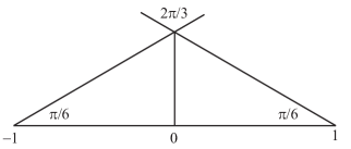
Figure 14. The Euclidean triangle $\Delta$.

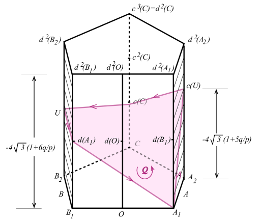
Figure 15. The fundamental domain in the Nil geometry $(X_{1},Q)$.

We can obtain explicitly the Nil geometry $(X_{1},Q)$ in $(\mathbb{T}_{p/q},\frac{6}{p+6q})$. Let $\Delta$ be the Euclidean triangle of Figure 14 . Because

$$d_{q/p}d_{q/p}=\left[\begin{array}[]{cccc}1&0&0&0\\ 0&1&0&0\\ 0&0&1&-4\sqrt{3}(6\frac{q}{p}+1)\\ 0&0&0&1\end{array}\right]$$

we can take the right prism with base $\Delta$ minus a small neighborhood of vertex $1$ and $-1$ and height $-4\sqrt{3}(6\frac{q}{p}+1)$ (Figure 15) as fundamental domain for the action of the group of isometries in the Nil geometry $(X_{1},Q)$, generated by $a_{q/p}$ and $b_{q/p}$ (or $c_{q/p}$ and $d_{q/p}$). The element $d_{q/p}^{2}$ identifies the two horizontal faces (bases) by translation. The element

$$d_{q/p}=\left[\begin{array}[]{cccc}-1&0&0&0\\ 0&-1&0&0\\ 0&0&1&-2\sqrt{3}(6\frac{q}{p}+1)\\ 0&0&0&1\end{array}\right]$$

identifies the two halfs of the front face producing a exceptional fibre $(2/1)$ as in the general case. The element

$$c_{q/p}=\left[\begin{array}[]{cccc}-\frac{1}{2}&-\frac{\sqrt{3}}{2}&0&\frac{1}{2}\\ \frac{\sqrt{3}}{2}&-\frac{1}{2}&0&\frac{\sqrt{3}}{2}\\ \frac{\sqrt{3}}{2}&\frac{1}{2}&1&-\frac{1}{2}\sqrt{3}(16\frac{q}{p}+3)\\ 0&0&0&1\end{array}\right]$$

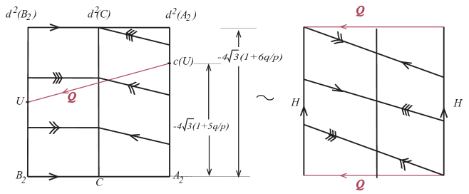
Figure 16. The exceptional fibre (3/1).

identifies the two back faces as it is shown in Figure 16, because

$$(c_{q/p}\circ\,b_{q/p})(A)=c_{q/p}\left(b_{q/p}\left(\begin{array}[]{c}1\\ 0\\ 0\\ 1\\ \end{array}\right)\right)=c_{q/p}\left(\begin{array}[]{c}-1\\ 0\\ -2\sqrt{3}(6\frac{q}{p}+1)\\ 1\\ \end{array}\right)=\left(\begin{array}[]{c}1\\ 0\\ -4\sqrt{3}(5\frac{q}{p}+1)\\ 1\\ \end{array}\right)$$

producing a $(3/1)$ exceptional fibre.

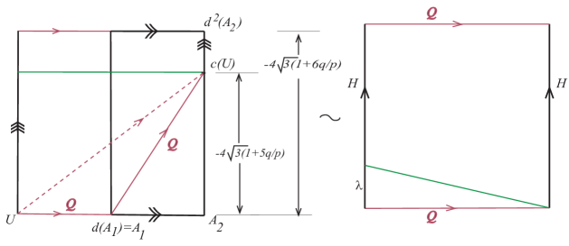
Figure 17. The exceptional fibre $(\frac{p}{q}+6)$.

The exceptional fibre coming from the collapsing of the leaves of the foliation in the boundary torus, depicted in Figure 17, is

$$\frac{4\sqrt{3}(1+6\frac{q}{p})}{-4\sqrt{3}(1+5\frac{q}{p})}=\frac{1+6\frac{q}{p}}{-(1+5\frac{q}{p})}.$$

The Seifert manifold is

(4.53) $$\begin{array}[]{l}(O\,o\,0|0;(2/1),(3/1),((1+6\frac{q}{p})/(-1-5\frac{q}{p})))=\\ (O\,o\,0|-1;(2/1),(3/1),((1+6\frac{q}{p})/(1+6\frac{q}{p}-1-5\frac{q}{p})))=\\ (O\,o\,0|-1;(2/1),(3/1),(6+\frac{q}{p})),\end{array}$$

which coincides with (4.40).

The length $\lambda$ of the singular curve (core of the surgery) is given in Theorem 4.1, namely $\lambda=\frac{6\theta-\pi}{m}$, where $m$ is the multiplicity of the exceptional fibre $\frac{p}{q}+6=\frac{p+6q}{q}=\frac{m}{n}$, $\gcd(m,n)=1$. Therefore, by (4.41)

$$\lambda=\frac{6\theta-\pi}{p+6q}=\frac{6\pi\left(\frac{1}{pr}-\frac{q}{p}\right)-\pi}{p+6q}=\frac{6\pi\left(1-qr\right)-pr\pi}{pr(p+6q)}=\frac{6\pi}{pr(p+6q)}-\frac{\pi}{p}.$$

Summarizing:

Theorem 4.2.

The conemanifold $(\mathbb{T}_{p/q},r)$, $p\neq 0$, has spherical geometry for

$$\frac{6}{5|p+6q|}<|r|<\frac{6}{|p+6q|},$$

Nil $X_{1}$ geometry for $|r|=\frac{6}{|p+6q|}$ and $\widetilde{SL(2,\mathbb{R})}$ geometry for

$$\frac{6}{|p+6q|}<|r|\leq\infty$$

The holonomy is generated by $a(\alpha,\theta)$ (3.20) and $b(\alpha,\theta)$ (3.21) where

$$\alpha=\frac{\pi}{r(p+6q)}\qquad\theta=\pi\left(\frac{1}{pr}-\frac{q}{p}\right)$$

when $|r|\neq\frac{6}{|p+6q|}$ and by $a_{q/p}$ and $b_{q/p}$ (4.46) if $|r|=\frac{6}{|p+6q|}$. The length of the singular knot is

(4.54) $$\lambda=\frac{6\pi}{pr(p+6q)}-\frac{\pi}{p}$$

∎

The following result adresses the remaining case $p=0$.

Theorem 4.3.

The conemanifold $(\mathbb{T}_{0},r)$, has Euclidean geometry for $r=1$; $H^{2}\times\mathbb{R}$ geometry for

$$1<|r|\leq\infty;$$

and $S^{2}\times\mathbb{R}$ geometry for

$$\frac{1}{5}<|r|<1.$$

Proof.

The trefoil knot is a fibred knot. The complement $C(\mathbb{T})$ of the trefoil knot is obtained from $F_{1,1}\times[0,1]$, where the punctured torus $F_{1,1}$ is a Seifert surface of the knot, by the identification $(x,0)=((h(x),1)$, where $h:F_{1,1}\longrightarrow F_{1,1}$ is an orientation preserving cyclic homeomorphism of order 6. The $0$-surgery on the knot consists in pasting a solid torus to $C(\mathbb{T})$ so that the boundary of the meridian disc in the torus is identified with the boundary of the Seifert surface. Therefore $\mathbb{T}_{0}=F_{1}\times[0,1]/(x,0)=((h^{\prime}(x),1)$, where $h^{\prime}:F_{1}\longrightarrow F_{1}$, extension of $h$, is a orientation preserving cyclic homeomorphism of order $6$.

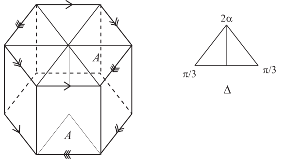
Figure 18. The manifold $\mathbb{T}_{0}$.

Figure 18 shows this manifold by identifications in a hexagonal right prism, where the base is the union of $6$ isosceles triangles $\Delta$ with angles $\pi/3$, $\pi/3$ and $2\alpha=2\pi/6r$. If the angle $\alpha$ is equal to $\pi/6$ ($r=1$) the hexagon lies on the Euclidean plane $E^{2}$ and the prism lies on $E^{2}\times\mathbb{R}$; if $\alpha<\pi/6$ ($1<|r|\leq\infty$) the hexagon is a 2-conemanifold in the hyperbolic plane $H^{2}$; and finally if $\pi/6<\alpha<5\pi/6$ ($\frac{1}{5}<|r|<1$) the hexagon is a 2-conemanifold in the 2-sphere $S^{2}$. ∎

One way to resume the different geometries in $(\mathbb{T}_{p/q},r)$, according to the different values of $p/q$ and $r$ is by creating a plot in $\mathbb{R}^{2}$ as follows.

Definition 4.1.

The lower limit of sphericity $l_{i}$ of the conemanifold $\mathbb{T}_{p/q}$ is equal to $\frac{6}{p+6q}$, and the upper limit of sphericity $l_{s}$ is equal to $\frac{6}{5(p+6q)}$.

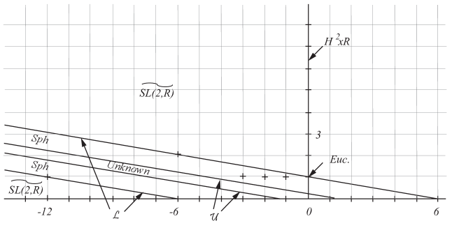
Figure 19. The plot $\mathcal{P}_{1}$.

In the plot $\mathcal{P}_{1}$ of Figure 19 the point $(rp,rq)$, with integer coordinates, where $gcd(p,q)=1$ and $q>0$, $r>0$ represents the surgery $p/q$ in the left-handed trefoil knot with conic angle $\beta=2\pi/r$, that is the cone manifold $(\mathbb{T}_{p/q},r)$.

Let $\varepsilon$ be the sign of $p+6q$. The set of lower limits is

$$\mathcal{L}=\left\{(x,y)\in\mathbb{R}^{2}:\;x=\frac{\varepsilon 6p}{p+6q},\;y=\frac{\varepsilon 6q}{p+6q}\right\}$$

and the set of upper limits is

$$\mathcal{U}=\left\{(x,y)\in\mathbb{R}^{2}:\;x=\frac{\varepsilon 6p}{5(p+6q)},\;y=\frac{\varepsilon 6q}{5(p+6q)}\right\}.$$

Both sets constitute a pair of straight lines depicted in Figure 19 and they divide the plane in regions with different geometries.

$$\begin{array}[]{c}\mathcal{L}=\left\{(x,y)\in\mathbb{R}^{2}:x+6y=6\varepsilon\right\}\\ \mathcal{U}=\left\{(x,y)\in\mathbb{R}^{2}:x+6y=\frac{6}{5}\varepsilon\right\}\end{array}$$

Points in $\mathcal{L}$ represent conemanifolds with Nil $X_{1}$ geometry. We do not know if the points in the region limited by the two straight lines in $\mathcal{U}$, including both lines, represent any geometric structure on the conemanifold $\mathbb{T}_{p/9}$, compatible with its as Seifert structure (fibres must be geodesics). An analogous plot is contained in [1].

4.2. Volume of the cone-manifold

To compute the volume of a family of spherical or hyperbolic cone manifold a normalized version of the metric should be used. The normalization for $X_{(S,S)}$, $S\neq 0$, consists in considering $|S|=1$. Then the metric matrix in Seifert coordinates, (3.1), for the normalized $X_{(S,S)}$, $S>0$, is the following

(4.55) $$Q_{1}((\mu,\nu,\theta)=\left[\begin{array}[]{ccc}\frac{\nu^{2}+1}{\left(1-\left(\mu^{2}+\nu^{2}\right)\right)^{2}}&-\frac{\mu\nu}{\left(1-\left(\mu^{2}+\nu^{2}\right)\right)^{2}}&\frac{\nu}{1-\left(\mu^{2}+\nu^{2}\right)}\\ &&\\ \ast&\frac{\mu^{2}+1}{\left(1-\left(\mu^{2}+\nu^{2}\right)\right)^{2}}&-\frac{\mu}{1-\left(\mu^{2}+\nu^{2}\right)}\\ &&\\ \ast&\ast&1\end{array}\right],$$

and for the normalized $X_{(S,S)}$, when $S<0$, is

(4.56) $$Q_{-1}((\mu,\nu,\theta)=\left[\begin{array}[]{ccc}\frac{\nu^{2}+1}{\left(1+\left(\mu^{2}+\nu^{2}\right)\right)^{2}}&-\frac{\mu\nu}{\left(1+\left(\mu^{2}+\nu^{2}\right)\right)^{2}}&-\frac{\nu}{1+\left(\mu^{2}+\nu^{2}\right)}\\ &&\\ \ast&\frac{\mu^{2}+1}{\left(1+\left(\mu^{2}+\nu^{2}\right)\right)^{2}}&\frac{\mu}{1+\left(\mu^{2}+\nu^{2}\right)}\\ &&\\ \ast&\ast&1\end{array}\right].$$

Their determinants are respectively

$$D(Q_{1})=\frac{1}{\left(1-\left(\mu^{2}+\nu^{2}\right)\right)^{4}},\quad\quad D(Q_{-1})=\frac{1}{\left(1+\left(\mu^{2}+\nu^{2}\right)\right)^{4}}$$

Suppose $S>0$. The volume form in the Seifert coordinates for the normalized $X_{(S,S)}$, ($X_{(1,1)}$), is

$$dv=\sqrt{|D(Q_{1})|}d\mu d\nu d\zeta=\frac{1}{\left(1-\left(\mu^{2}+\nu^{2}\right)\right)^{4}}d\mu d\nu d\zeta$$

Therefore

$$V(\mathbb{T}_{p/q},r) = \int_{D(\alpha,\theta)}dv=\int_{D(\alpha,\theta)}\frac{1}{\left(1-\left(\mu^{2}+\nu^{2}\right)\right)^{4}}d\mu d\nu d\zeta$$

$$= \int_{0}^{\zeta_{0}}d\zeta\int_{\Delta}\frac{1}{\left(1-\left(\mu^{2}+\nu^{2}\right)\right)^{4}}d\mu d\nu=\zeta_{0}\times\frac{1}{4}\text{Area of }\Delta$$

where $\zeta_{0}$ and $\Delta$ are, respectively, the height and the base of $D(\alpha,\theta)$. The geometry in the base is hyperbolic. By construction of the fundamental domain $D(\alpha,\theta)$, the base is a hyperbolic triangle with angles $2\pi/3,\alpha,\alpha$, and the height $\zeta_{0}$ is $|6\theta-\pi|$, where (4.41)

$$\alpha=\frac{\pi}{r(p+6q)}\qquad\theta=\frac{\pi(1-qr)}{pr}$$

Therefore

$$\text{Area of }\Delta=\pi-2\pi/3-2\alpha=\pi/3-\frac{2\pi}{r(p+6q)}=\frac{\pi r(p+6q)-6\pi}{3r(p+6q)}$$

$$V(\mathbb{T}_{p/q},r)=\left|\frac{6\pi(1-qr)}{pr}-\pi\right|\left(\frac{\pi(r(p+6q)-6\pi)}{3r(p+6q)}\right)\frac{1}{4}=\left|-\frac{\pi^{2}(pr+6qr-6)^{2}}{12pr^{2}(p+6q)}\right|.$$

Suppose $S<0$. The volume form in the Seifert coordinates for the normalized $X_{(S,S)}$, ($X_{(-1,-1)}$), is

$$dv=\sqrt{|D(Q_{-1})|}d\mu d\nu d\zeta=\frac{1}{\left(1+\left(\mu^{2}+\nu^{2}\right)\right)^{4}}d\mu d\nu d\zeta$$

Therefore

$$V(\mathbb{T}_{p/q},r) = \int_{D(\alpha,\theta)}dv=\int_{D(\alpha,\theta)}\frac{1}{\left(1+\left(\mu^{2}+\nu^{2}\right)\right)^{4}}d\mu d\nu d\zeta$$

$$= \int_{0}^{\zeta_{0}}d\zeta\int_{\Delta}\frac{1}{\left(1+\left(\mu^{2}+\nu^{2}\right)\right)^{4}}d\mu d\nu=\zeta_{0}\times\frac{1}{4}\text{Area of }\Delta$$

where $\zeta_{0}$ and $\Delta$ are respectively the height and the base of $D(\alpha,\theta)$. The geometry in the base is spherical. By construction of the fundamental domain $D(\alpha,\theta)$, the base is a spherical triangle with angles $2\pi/3,\alpha,\alpha$, and the height $\zeta_{0}$ is $\left|6\theta-\pi\right|$, where (4.41)

$$\alpha=\frac{\pi}{r(p+6q)}\qquad\theta=\frac{\pi(1-qr)}{pr}$$

Therefore

$$\text{Area of }\Delta=2\pi/3+2\alpha-\pi=\frac{2\pi}{r(p+6q)}-\pi/3=\frac{6\pi-\pi(r(p+6q))}{3r(p+6q)}$$

$$V(\mathbb{T}_{p/q},r)=\left|\frac{6\pi(1-qr)}{pr}-\pi\right|\left(\frac{6\pi-\pi(r(p+6q))}{3r(p+6q)}\right)\frac{1}{4}=\left|\frac{\pi^{2}(pr+6qr-6)^{2}}{12pr^{2}(p+6q)}\right|.$$

Remark 4.1.

Observe that the volume $V(\mathbb{T}_{p/q},r)$, as could be suggested by the construction, is not the product of the area of the base by the height $\zeta_{0}$. There is a correcting factor of $(1/4)$ because the geometry is a twisted geometry.

The following examples offer the volume of the conemanifolds represented by some points in the plot $\mathcal{P}_{1}$.

Example 1. $(-1,1)\in\mathcal{P}_{1}$, $(K=1,\,p=-1,\,q=1,\,r=1$). Spherical geometry.

$$V(\mathbb{T}_{-1},1)=\frac{2\pi^{2}}{120}$$

This manifold is the Poincaré spherical manifold, obtained by $(-1)$-surgery in the left-handed trefoil knot. This manifold is the quotient of the sphere $\mathbb{S}^{3}$ by the binary icosahedral group $I\ast$, group with $120$ elements. The volume of $\mathbb{S}^{3}$ is $2\pi^{2}$.

Example 2. $(5,0)\in\mathcal{P}_{1}$, $(K=1,\,p=1,\,q=0,\,r=5)$. Spherical geometry.

$$V(\mathbb{T}_{\infty},5)=\frac{2\pi^{2}}{600}=\frac{2\pi^{2}}{120}\left/5\right.$$

This result is coherent with the fact that the $5$-fold cyclic covering of $\mathbb{S}^{3}$ branched over the trefoil knot is the Poincaré spherical manifold.

Example 3. $(2,0)\in\mathcal{P}_{1}$, $(K=1,\,p=1,\,q=0,\,r=2)$. Spherical geometry.

$$V(\mathbb{T}_{\infty},2)=\frac{2\pi^{2}}{6}$$

This result is coherent with the fact that the double covering of $\mathbb{S}^{3}$ branched over the trefoil knot is the lens $L(3,1)$ which has $\mathbb{S}^{3}$ as its universal cover with $3$ sheets and therefore it has volume $\frac{2\pi^{2}}{3}=2V(\mathbb{T}_{\infty},2)$.

Example 4. $(3,0)\in\mathcal{P}_{1}$, $(K=1,\,p=1,\,q=0,\,r=3)$. Spherical geometry.

$$V(\mathbb{T}_{\infty},3)=\frac{2\pi^{2}}{24}$$

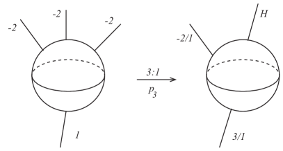
Figure 20. The covering $p_{3}:(Oo0|1;-2,-2,-2)\longrightarrow(Oo0|-1;2/1,3/1)$.

In Figure 20 is depicted a scheme (compare [5, Figure 12 p.146]) of the covering

$$p_{3}:(Oo0|1;-2,-2,-2)\longrightarrow(Oo0|-1;2/1,3/1)$$

branched over an ordinary fibre $H$ which is a trefoil knot. In Figure 20 we have depicted the bases (both $\mathbb{S}^{2}$) of the Seifert structures involved together with the exceptional fibres and an ordinary fibre.

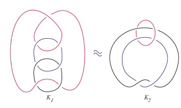
Figure 21. The knots $K_{1}$ and $K_{2}$.

The map $p_{3}$ is the 3-fold cyclic covering of $\mathbb{S}^{3}$ branched over the trefoil knot. On the other hand the Seifert manifolds $(Oo0|1;-2,-2,-2)$ and $(On1|2)$ are the 2-fold covering of $\mathbb{S}^{3}$ branched over the knots $K_{1}$ and $K_{2}$, depicted in Figure 21 respectively ([4] and [5]). Figure 21 proves that the links $K_{1}$ and $K_{2}$ are different diagrams of the same knot, therefore the Seifert manifolds are equal:

$$(Oo0|1;-2,-2,-2)=(On1|2).$$

This is the quaternionic space, having $\mathbb{S}^{3}$ as universal covering with $8$ sheets. Note that the group acting in $\mathbb{S}^{3}$ with quotient the quaternionic space $(On1|2)$ is the binary dihedral $<2\,2\,2>$ with 24 elements. Therefore $(\mathbb{T}_{\infty},3)$ is the quotient of $\mathbb{R}P^{3}$ by the action of the tetrahedral group ([5]).

Example 5. $(4,0)\in\mathcal{P}_{1}$, $(K=1,\,p=1,\,q=0,\,r=4)$. Spherical geometry.

$$V(\mathbb{T}_{\infty},4)=\frac{2\pi^{2}}{96}$$

The universal covering of $(\mathbb{T}_{\infty},4)$ factors through the octahedral manifold $\mathbb{S}^{3}/T^{\ast}$, where $T^{\ast}$ is the binary tetrahedral group, and also, through the manifold $(Oo0|-4)=(Oo0|0;\overset{8}{\underbrace{1,...,1}},\overset{12}{\overbrace{-1,...,-1}})$.

$$\mathbb{S}^{3} \overset{24:1}{\longrightarrow} \mathbb{S}^{3}/T^{\ast}=(Oo0|-2;3,3,3,3)$$

$${}_{4:1}\downarrow {}_{96:1}\searrow \downarrow{}_{4:1}$$

$$(Oo0|-4) \overset{24:1}{\longrightarrow} (\mathbb{T}_{\infty},4)=(Oo0|0;-2,3)=\mathbb{S}^{3}$$

Example 6. $(\infty,0)\in\mathcal{P}_{1}$, $(p=1,\,q=0,\,r=\infty)$. $\widetilde{SL(2,\mathbb{R})}$ geometry.

$$V(\mathbb{T}_{\infty},\infty)=\frac{\pi^{2}}{12}$$

The geometry in the conemanifolds $(\mathbb{T}_{\infty},r)$, $r>6$ is $\widetilde{SL(2,\mathbb{R})}$. The volume of $(\mathbb{T}_{\infty},\infty)$ will be the limit of $V(\mathbb{T}_{\infty},r)$, $r\to\infty$:

$$V(\mathbb{T}_{\infty},\infty)=\lim_{r\to\infty}V(\mathbb{T}_{\infty},r)=\lim_{r\to\infty}\frac{\pi^{2}(-6+r)^{2}}{12r^{2}}=\frac{\pi^{2}}{12}$$

Example 7. $(6,0)\in\mathcal{P}_{1}$, $(p=1,\,q=0,\,r=6)$. $X_{1}$ geometry

$(\mathbb{T}_{\infty},6)$ is the Seifert manifold $(Oo0|-1;(2/1),(3/1),(6/1))$ according to (4.53). The singular fibre is the core of the surgery (here the trefoil knot) with angle $\beta=2\pi/6$. The $6$-fold covering of $\mathbb{S}^{3}$ branched over the trefoil knot is the Seifert manifold $(Oo1|1)$ ([4])

$$V(\mathbb{T}_{\infty},6)=\lim_{r\rightarrow 6}V(\mathbb{T}_{\infty},r)=\lim_{r\rightarrow 6}\frac{\pi^{2}(-6+r)^{2}}{12r^{2}}=0$$

.

4.3. Plotting the geometric structures on the manifolds obtained by surgery on the trefoil knot

We are studying cone-manifold structures in manifolds obtained by Dehn-surgery on the Trefoil knot in $\mathbb{S}^{3}$. These manifolds are Seifert manifolds with geometric structure and with the core of the surgery as singular set. It seems natural to adopt the following new notation.

Notation 1.

Let

$$S(m,n)=\left(Oo0|-1;(2,1),(3,1),(m,n)\right)\qquad m\geq 0$$

be the Seifert manifold $\left(Oo0|-1;(2,1),(3,1),(\frac{m}{r},\frac{n}{r})\right)$, where $r=\gcd(m,n)$, with conic singularity along the exceptional fibre $(\frac{m}{r},\frac{n}{r})$ of angle $2\pi/r$.

Recall that the holonomy of $S(m,n)$ is generated by $a(\alpha,\theta)$ (3.20) and $b(\alpha,\theta)$ (3.21), where

$$\left\{\begin{array}[]{c}\frac{2\pi}{r}=2\alpha\frac{m}{r}\\ \\ \frac{6\theta-\pi}{\theta-\alpha}=\frac{m}{n}\end{array}\right.$$

if $\alpha\neq\pi/6$. The geometry is $\widetilde{SL(2,\mathbb{R})}$ for $0\leq\alpha<\frac{\pi}{6}$; Nil for $\alpha=\frac{\pi}{6}$; and spherical for $\frac{\pi}{6}<\alpha<\frac{5\pi}{6}$.

Because

$$\frac{m}{n}=6+\frac{p}{q}=\frac{6q+p}{p}\quad\Longrightarrow\quad 8\frac{q}{p}+1=(\frac{m+2n}{m-6n}),$$

where $p/q$ is the datum of the surgery, the holonomy (4.46) for $\alpha=\frac{\pi}{6}$ is given by the matrices

$$a_{m/n} = \left[\begin{array}[]{cccc}\frac{1}{2}&-\frac{\sqrt{3}}{2}&0&\frac{1}{2}\\ \frac{\sqrt{3}}{2}&\frac{1}{2}&0&-\frac{\sqrt{3}}{2}\\ \frac{\sqrt{3}}{2}&-\frac{1}{2}&1&-\frac{1}{2}\sqrt{3}(\frac{m+2n}{m-6n})\\ 0&0&0&1\end{array}\right]$$

$$b_{m/n} = \left[\begin{array}[]{cccc}\frac{1}{2}&-\frac{\sqrt{3}}{2}&0&-\frac{1}{2}\\ \frac{\sqrt{3}}{2}&\frac{1}{2}&0&\frac{\sqrt{3}}{2}\\ -\frac{\sqrt{3}}{2}&\frac{1}{2}&1&-\frac{1}{2}\sqrt{3}(\frac{m+2n}{m-6n})\\ 0&0&0&1\end{array}\right]$$

With the notation $S(m,n)$

$$\left(\mathbb{T}_{p/q},r\right) = S(r(6q+p),rq)$$

$$S(m,n) = \left(\mathbb{T}_{(m-6n)/n},m.c.d.(m,n)\right)$$

$$\alpha = \frac{\pi}{m}$$

$$\theta = \pi\frac{n-1}{6n-m}$$

$$V(S(m,n)) = -\frac{\pi^{2}}{S}\frac{(m-6)^{2}}{12m(m-6n)}$$

$$V(S(\infty m,\infty n)) = -\frac{\pi^{2}}{S}\frac{m}{12(m-6n)}$$

$$\left\{\begin{array}[]{c}6<m\leq\infty\\ m=6\\ \frac{6}{5}<m<6\end{array}\right\}\quad\text{geometry}\quad\left\{\begin{array}[]{c}\widetilde{{SL(2,\mathbb{R})}}\\ \text{Nil}\\ \text{spherical}\end{array}\right\}$$

One of the advantages of using the notation $S(m,n)$ is that the information about the different geometries on the same Seifert manifold can best be seen in the following plot $\mathcal{P}_{2}$ (Figure 22), written in the spirit of Thurston (see [7, p. 4.21]). The points in the plot bearing the symbol $\blacklozenge$ correspond to points $(x,y)$ such that $x$ and $y$ are non-negative integers with $\gcd(x,y)=1$. They represent the manifolds $S(x,y)$ with no singularity. The points in the line $x/y$ connecting the origin $(0,0)$ with the point $(x,y)$ represent $S(x\times r,y\times r)$. This is a cone-manifold with underlying $3$-manifold the common Seifert manifold $S(x,y)$, but the cone angle $2\pi/r$ varies from zero to infinity. The left vertical dashed line $\mathcal{U}$ corresponds to the set of upper limits $\mathcal{U}$ in the plot $\mathcal{P}_{1}$ and it separates the left region, with unknown, if any, geometry compatible with the Seifert structure in the sense that fibres must be geodesics, from the region whose points represent spherical geometry. Points in the right vertical dashed line $\mathcal{L}$, which correspond to the lower limits $\mathcal{L}$ in plot $\mathcal{P}_{1}$, represent Nil geometry and it separates the region whose points represent spherical geometry from the region whose points represent $\widetilde{{SL(2,\mathbb{R})}}$ geometry.

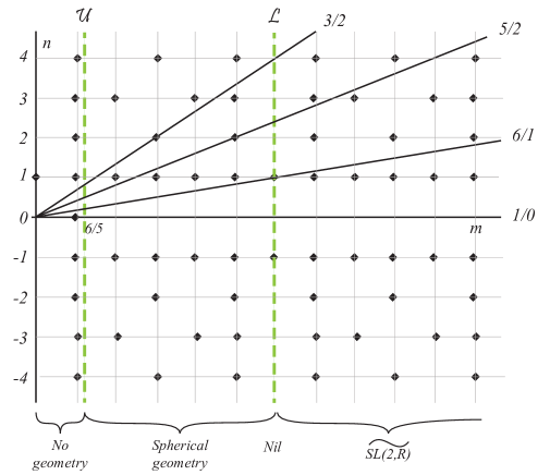
Figure 22. The plot $\mathcal{P}_{2}$.

Definition 4.2.

The limit of sphericity $\gamma_{e}$ of the Seifert manifold $S(x,y)$ is the cone angle of the cone-manifold structure corresponding to the intersection point $\mathcal{U}\cap(x/y)$.

The Nil angle $\gamma_{N}$ of the Seifert manifold $S(x,y)$ is the cone angle of the cone-manifold structure corresponding to the intersection point $\mathcal{L}\cap(x/y)$. Their value as a function of $(x,y)$ is the following

$$\gamma_{e}=\frac{5x\pi}{3}\quad\quad\gamma_{N}=\frac{x\pi}{3}$$

Next we summarize some affirmations that are deduced easily from the plot $\mathcal{P}_{2}$.

Summary 2.

Let $x$ and $y$ be non-negative integers with $\gcd(x,y)=1$.

• The geometric cone-manifold structure with cone angle $\gamma$ in $S(x,y)$ is spherical for $\gamma_{e}>\gamma>\gamma_{N}$, Nil for $\gamma=\gamma_{N}$, and $\widetilde{{SL(2,\mathbb{R})}}$ for $\gamma_{N}>\gamma$.

• The limit of sphericity $\gamma_{e}$ is equal to five times the Nil angle $\gamma_{N}$

• There exits infinity many non-singular Nil geometric structures:
  $S(6,y)=\left(\mathbb{T}_{(6-6y)/y},1\right)$, where $\gcd(6,y)=1$.

• There exits infinity many Nil orbifold geometric structures:

  1. $S(6,3y)=\left(\mathbb{T}_{(2-6y)/y},3\right)$, where $\gcd(2,y)=1$,

  2. $S(6,2y)=\left(\mathbb{T}_{(3-6y)/y},2\right)$, where $\gcd(3,y)=1$.

• If $\left(\mathbb{T}_{p/q},r\right)=S(r(6q+p),rq)$ has a spherical orbifold structure, then $2\leq r\leq 5$.

Lets analyze some points in the region $m\in[0,6/5]$. The vertical axis $x=0$ yields $S(0,y)$, corresponding to the manifold $L(2,1)\sharp L(3,1)$ with no geometry. Between this axis and the vertical line $m=6/5$ are placed the Seifert manifolds (no singular)

$$S(1,n)=(Oo0|-1;(2,1),(3,1),(1,n))=(Oo0|n-1;(2,1),(3,1))$$

which are the lens $-L(6n-1,2n-1)$ for $n\neq 0$, and $\mathbb{S}^{3}$ for $n=0$. It is known that these Seifert manifolds (lens spaces) support spherical geometry but the fibre $(1,n)$ of the Seifert fibration $(Oo0|-1;(2,1),(3,1),(1,n))$ is not a geodesic of that geometry. For instance, in $S(1,0)=\mathbb{S}^{3}$, the fibre $(1,0)$ is a regular fibre, the left Trefoil knot, which obviously is not a geodesic in $\mathbb{S}^{3}$. Recall that we are studying geometric structures in the Seifert manifold $S(x,y)$ such that the fibre $(x,y)$ is a geodesic (singular or not), that is Seifert geometric conemanifolds.

References

- [1] S. Kojima. A construction of geometric structures on Seifert fibered spaces. J. Math. Soc. Japan, 36 n 3: 483–495, 1984.
- [2] M. T. Lozano, and J. M. Montesinos-Amilibia. On the degeneration of some 3-manifold geometries via unit groups of quaternion algebras. Preprint, 2014.
- [3] Y. Matsumoto, and J. M. Montesinos-Amilibia. A proof of Thurston’s uniformization theorem of geometric orbifolds. Tokyo J. Math., 14 n 1:181–196, 1991.
- [4] J. M. Montesinos-Amilibia. Seifert manifolds that are ramified two-sheeted cyclic coverings. (Spanish) Bol. Soc .Mat. Mexicana, (2) 18 :1–32, 1973.
- [5] J. M. Montesinos-Amilibia. Classical tessellations and three-manifolds. Springer-Verlag, Berlin, 1987 xviii+230 pp.
- [6] H. Seifert. Topologie dreidimensionaler gefaserter räume. Acta Math., 60:147–238, 1933.
- [7] W.P. Thurston. The geometry and topology of three-manifolds. Princeton University Lectures, 1976-1977, available at htt://library.msri.org/books/gt3m/
- [8] W. P. Thurston. Three-dimensional geometry and topology. Vol 1. Edited by Silvio Levy. Princeton Mathematical Series, 35. Princeton University Prtess. Princeton, NJ, 1997. x+311 pp.