Distributed Storage Allocations for Neighborhood-based Data Access

Abstract

We introduce a neighborhood-based data access model for distributed coded storage allocation. Storage nodes are connected in a generic network and data is accessed locally: a user accesses a randomly chosen storage node, which subsequently queries its neighborhood to recover the data object. We aim at finding an optimal allocation that minimizes the overall storage budget while ensuring recovery with probability one. We show that the problem reduces to finding the fractional dominating set of the underlying network. Furthermore, we develop a fully distributed algorithm where each storage node communicates only with its neighborhood in order to find its optimal storage allocation. The proposed algorithm is based upon the recently proposed proximal center method–an efficient dual decomposition based on accelerated dual gradient method. We show that our algorithm achieves a $(1+\epsilon)$-approximation ratio in $O(d_{\mathrm{max}}^{3/2}/\epsilon)$ iterations and per-node communications, where $d_{\mathrm{max}}$ is the maximal degree across nodes. Simulations demonstrate the effectiveness of the algorithm.

I Introduction

With distributed (coded) storage allocation problems [1, 2], one aims to store a data object over $N$ storage nodes, such that the tradeoff between redundancy (total amount of storage) and reliability of accessing the object is balanced in an optimal way. A standard instance of the problem is as follows. Store a unit size data object $D$ over $N$ nodes, such that each node $i$ stores an amount of $x_{i}$ storage encoded from object $D$. At a later time, a data collector–user accesses a fixed number $r$, $r<N$, of randomly chosen nodes, and attempts to recover $D$. Assuming a maximum distance separable (MDS) coding is used, the recovery is successful if the overall amount of storage across the selected nodes is at least equal in size to $D$. Then, the goal is to optimize the $x_{i}$’s such that the total storage $\sum_{i=1}^{N}x_{i}$ is minimized, while the recovery probability exceeds a prescribed level.

In this paper–motivated by applications like cloud storage systems, peer-to-peer (P2P) networks, sensor networks or caching in small-cell cellular networks–we introduce a new, neighborhood-based data access model in the context of distributed coded storage allocation. We assume that the $N$ storage nodes are interconnected with links and constitute a generic network. A user (e.g., smartphone, sensor, P2P client application) accesses a randomly chosen node $i$. Subsequently, node $i$ contacts its one-hop neighbors, receives their coded storage, and, combined with its own storage, passes the aggregate storage to the user, which finally attempts the recovery. Then, our goal is to minimize $\sum_{i=1}^{N}x_{i}$ such that the recovery probability is one.

We show that the resulting problem is a fractional dominating set (FDS) linear program (LP), e.g., [3], and hence can be efficiently solved via standard LP solvers. However, we are interested in solving FDS in a fully distributed way, whereby nodes over iterations exchange messages with their neighbors in the network with the aim of finding their optimal local allocations. Several distributed algorithms to solve FDS, and, more generally, fractional packing and covering LPs, have been proposed,   e.g., [4]-[7]. However, advanced dual decomposition techniques based on the Lagrangian dual, proved useful in many distributed applications, have not been sufficiently explored. In this paper, to solve FDS in a fully distributed way, we apply and modify the proximal center method proposed in [8]–an efficient dual decomposition based on accelerated Nesterov gradient method. We show that the resulting method is competitive with existing, primal-based approaches. Assuming that all nodes know $d_{\mathrm{max}}$ and $\epsilon$ beforehand ($d_{\mathrm{max}}$ the maximal degree across nodes, and $\epsilon$ the required accuracy), we show that the algorithm achieves a $(1+\epsilon)$-approximation ratio in $O(d_{\mathrm{max}}^{3/2}/\epsilon)$ iterations $k$–more precisely–$O(d_{\mathrm{max}}^{3/2}/\epsilon)$ per-node scalar communications and $O(d_{\mathrm{max}}^{5/2}/\epsilon)$ per-node elementary operations (computational cost). This matches the best dependence on $\epsilon$ among existing solvers [4]-[7], [5, 10], proposed for FDS (or fractional packing/covering). Furthermore, the algorithm’s iterates are feasible (satisfy problem constraints) at all iterations. Simulations demonstrate that our algorithm converges much faster than a state-of-the-art distributed solver [6] on moderate-size networks ($N=100-400$.) With respect to [8] (which considers generic convex programs), we introduce here a novel, simple way of maintaining feasibility along iterations by exploiting the FDS problem structure. Further, exploiting structure, the results in [11], and primal-dual solution bounds derived here, we improve the dependence on the underlying network (on $N,d_{\mathrm{max}}$) with respect to a direct application of the generic results in [8].

Summarizing, our main contributions are two-fold. First, we introduce a new, neighborhood-based data access model for distributed coded storage allocation–the model well-suited in many user-oriented applications for distributed networked storage–and we show that the corresponding optimization problem reduces to FDS. Second, we solve the coded storage allocation problem (FDS) where storage nodes search for their optimal local allocations in a fully distributed way by applying and modifying the dual-based proximal center method. We establish the method’s convergence and complexity guarantees and show that it compares favorably with a state-of-the art method on moderate-size networks.

I-A Literature review, paper organization, and notation

We now briefly review the literature to further contrast our paper with existing work. Neighborhood-based data access has been previously considered in the context of replica placement, e.g., [12]. Therein, one wants to replicate the raw object $D$ across network such that it is reliably accessible through a neighborhood of any node. In contrast, we consider here the coded storage. Mathematically, replica placement corresponds to the integer dominating set problem (known to be NP hard), while coded allocation studied here translates into FDS (solvable in polynomial time).

We now contrast our distributed algorithm for FDS with existing methods. The literature usually considers more general fractional packing/covering problems, , e.g., [4]-[7], [5, 10], and we hence specialize their results to FDS. References [4]-[7] develop distributed algorithms, with the required number of iterations (per-node communications) that depends on $\epsilon$ (at least) as $1/\epsilon^{4}$, and on $N$ as $(\log N)^{O(1)}$ (poly-logarithmically). The algorithm in [6] enjoys a stateless property (see [6] for the definition of the property), while our algorithm is not stateless (e.g., it requires a global clock). References [9, 10] develop algorithms with a better dependence on $\epsilon$ than $1/\epsilon^{4}$. They are not concerned with developing fully distributed algorithms. The algorithm in [10] requires $O(N\log N/\epsilon^{2})$ iterations, while [9] takes $O(\sqrt{Nd_{\mathrm{max}}\log N}/\epsilon)$ iterations. In summary, among existing solvers [4]-[7], [5, 10], our algorithm matches the best dependence on $\epsilon$, is fully distributed, can achieve arbitrary accuracy, is not stateless, and has in general worse dependence on $N$.

The remainder of the paper is organized as follows. The next paragraph introduces notation. Section II gives the system model with neighborhood-based data access and formulates the distributed coded storage allocation problem as a FDS. Section III presents the proximal center distributed algorithm to solve FDS and states our results on its performance. Section IV gives the algorithm derivation and proofs. Section V shows simulation examples. Finally, we conclude in Section VI.

Throughout, we use the following notation. We denote by: ${\mathbb{R}}^{N}$ the $N$-dimensional real space; ${\mathbb{R}}^{N}_{+}$ the set of $N$-dimensional vectors with non-negative entries; $a_{i}$ the $i$-th entry of vector $a$; $A_{ij}$ the $(i,j)$-th entry of matrix $A$; $0$ and $\mathbf{1}$ the column vector with, respectively, zero and unit entries; $h_{i}$ the $i$-th canonical vector;$\|\cdot\|=\|\cdot\|_{2}$ the Euclidean norm of a vector; $\nabla g(y)$ the gradient at point $y$ of a differentiable function $g:\,{\mathbb{R}}^{N}\rightarrow\mathbb{R}$; $|S|$ cardinality of set $S$; and $\mathcal{I}_{\mathcal{E}}$ the indicator of event $\mathcal{E}$. For two vectors $a,b\in{\mathbb{R}}^{N}$, the inequality $a\leq b$ is understood component-wise. For a vector $a$, $[a]_{+}$ is a vector with the $i$-th entry equal to $\max\{0,a_{i}\}$ (Similarly, for a scalar $c$, $[c]_{+}=\max\{0,c\}$.) Next, $\mathcal{P}_{[0,1]}(c)$ is the projection of scalar $c$ on the interval $[0,1]$, i.e., $\mathcal{P}_{[0,1]}(c)=c$, for $c\in[0,1]$; $\mathcal{P}_{[0,1]}(c)=0$, for $c<0$; and $\mathcal{P}_{[0,1]}(c)=1$, for $c>1.$ Finally, for two positive sequences $\eta_{n}$ and $\chi_{n}$, $\eta_{n}=O(\chi_{n})$ means that $\limsup_{n\rightarrow\infty}\frac{\eta_{n}}{\chi_{n}}<\infty$.

II Problem model

We consider coded distributed storage of a unit-size data object $D$ over a network of $N$ storage nodes. Each storage node $i$ stores a coded portion of $D$ of size $x_{i}$, $x_{i}\in[0,1]$. For example, nodes can utilize random linear coding, where $D$ is divided into $M$ disjoint parts; node $i$ stores $x_{i}\times M$ random linear combinations of the parts of $D$, e.g., [1] (ignoring the rounding of $x_{i}\times M$ to closest integer). We assume that storage nodes constitute an arbitrary undirected network $\mathcal{G}=(\mathcal{N},E)$, where $\mathcal{N}$ is the set of $N$ storage nodes, and $E$ is the set of communication links between them. Denote by $\Omega_{i}$ the one-hop closed neighborhood set of node $i$ (including $i$), and by $d_{i}=|\Omega_{i}|$ its degree. Also, let $A$ be the $N\times N$ symmetric adjacency matrix associated with $\mathcal{G}$: $A_{ii}=1$, $\forall i$; and, for $i\neq j$, $A_{ij}=1$ if $\{i,j\}\in E$, and $A_{ij}=0$, else.

A user accesses node $i$ with probability $p_{i}>0$. Upon the user’s request, node $i$ contacts its neighbors $j\in\Omega_{i}\setminus\{i\}$, and they transmit their coded storage to $i$. Hence, afterwards, node $i$ has available the amount of storage equal to $\sum_{j\in\Omega_{i}}x_{j}$. If a MDS coding scheme is used, the recovery of object $D$ is successful if $\sum_{j\in\Omega_{i}}x_{j}\geq 1$. Thus, the probability of successful recovery equals: $\sum_{i=1}^{N}p_{i}\,\mathcal{I}_{\{\sum_{j\in\Omega_{i}}x_{j}\geq 1\}}.$ We aim at minimizing the total storage $\sum_{i=1}^{N}x_{i}$ such that the probability of recovery is one: $\sum_{i=1}^{N}p_{i}\,\mathcal{I}_{\{\sum_{j\in\Omega_{i}}x_{j}\geq 1\}}=1$. This translates into FDS, which, letting $x:=(x_{1},...,x_{N})^{\top}$, in compact form, can be written as:

$$\begin{array}[+]{ll}\mbox{minimize}&{\mathbf{1}}^{\top}x\\ \mbox{subject to}&A\,x\geq\mathbf{1}\\ &x\geq 0.\end{array}$$ (1)

Clearly, (1) has a non-empty constraint set (e.g., take $x=\mathbf{1}$), and a solution exists. Denote by $x^{\star}$ a solution to (1).

In this paper, for simplicity, we focus on one-hop neighborhood data access model. Our framework straightforwardly generalizes to $\ell$-hop neighborhood data access, $\ell>1$, where a user attempts the recovery based on the $\ell$-hop neighborhood of the queried node. Formally, in (1) we replace $A$ with the adjacency matrix $A_{\ell}$ of graph $\mathcal{G}_{\ell}=(\mathcal{N},E_{\ell})$, where $E_{\ell}$ contains all pairs $\{i,j\}$ such that there exists a path of length not greater than $\ell$ between them.

We are interested in developing a distributed, iterative algorithm, where nodes exchange messages with their one-hop neighbors in the network, so that the allocation $x$ produced by the algorithm satisfies a $(1+\epsilon)$ approximation ratio: $\frac{1^{\top}x}{1^{\top}x^{\star}}\leq 1+\epsilon$, where $\epsilon>0$ is given beforehand. In this paper, we focus on how to determine the (nearly optimal) amount of coded storage $x_{i}$ at each node $i$. Once the amounts $x_{i}$’s are determined, in an actual implementation, nodes perform coding and actually store the coded content; this is not considered here.

III Distributed algorithm for coded storage allocation

III-A The algorithm

We apply the proximal center method [8] to solve the coded storage allocation problem (1). The algorithm is based on the dual problem of a regularized version of (1), and on the Nesterov gradient algorithm. With respect to [8], we choose the dual step-size differently; the step-size choice arises from the analysis here and in [11]. Also, we modify the method to produce feasible primal updates at every iteration. (See Section IV for the algorithm derivation.)

The algorithm is iterative, and all nodes operate in synchrony. We denote the iterations by $k=0,1,2,...$ Each node $i$ maintains over iterations $k$ its current (scalar) solution estimate $x_{i}^{(k)}$, where $x_{i}^{(k)}$ remains feasible to (1), and the auxiliary (scalar) variables: $\lambda_{i}^{(k)}$, $\mu_{i}^{(k)}$, $\widehat{x}_{i}^{(k)}$, and $z_{i}^{(k)}$, and $\overline{x}_{j}^{(k)}$, $\forall j\in\Omega_{i}.$ (Node $i$ also has $z_{i}^{(-1)}=0.$) Let $1+\epsilon$ be the approximation ratio that nodes want to achieve, $\epsilon>0$. Our algorithm has parameters $\alpha,\delta>0$, set to: $\delta=\epsilon$, and $\alpha=\frac{\delta}{2(d_{\mathrm{max}}+1)^{2}}$. (See also Section IV.) The algorithm is presented in Algorithm 1. We assume that all nodes know beforehand the quantities $d_{\mathrm{max}}$ and $\epsilon.$

1:  (Initialization) Each node $i$ sets $k=0$, $\lambda_{i}^{(0)}=0$, $z_{i}^{(-1)}=0$, $\delta=\epsilon$, and $\alpha=\frac{\delta}{2(d_{\mathrm{max}}+1)^{2}}$.

2:  For $k=0,1,2,...$, perform steps $3$–$6$:

3:  If $k\geq 1$, each node $i$ transmits $\lambda_{i}^{(k)}$ to all $j\in{\Omega_{i}}\setminus\{i\}$, and receives $\lambda_{j}^{(k)}$, $\forall j\in{\Omega_{i}}\setminus\{i\}$ (if $k=0$ this step is skipped.)

4:  Each node $i$ computes:

$$\widehat{x}_{i}^{(k)}=\mathcal{P}_{[0,1]}\left(\frac{1}{\delta}(\sum_{j\in{\Omega_{i}}}\lambda_{j}^{(k)}-1)\right)$$ (2)

5:  Each node $i$ transmits $\widehat{x}_{i}^{(k)}$ to all $j\in{\Omega_{i}}\setminus\{i\}$, and receives $\widehat{x}_{j}^{(k)}$, $\forall j\in{\Omega_{i}}\setminus\{i\}$.

6:  Each node $i$ computes:

$$z_{i}^{(k)} = z_{i}^{(k-1)}+\frac{k+1}{2}\left(1-\sum_{j\in{\Omega_{i}}}\widehat{x}_{j}^{(k)}\right)$$ (3)

$$\mu_{i}^{(k)} = \left[\,\lambda_{i}^{(k)}+\alpha\left(1-\sum_{j\in{\Omega_{i}}}\widehat{x}_{j}^{(k)}\right)\,\right]_{+}$$ (4)

$$\lambda_{i}^{(k+1)} = \frac{k+1}{k+3}\,\mu_{i}^{(k)}+\frac{2}{k+3}\alpha\left[z_{i}^{(k)}\right]_{+}$$ (5)

$$\overline{x}_{j}^{(k)} = \frac{k}{k+2}\overline{x}_{j}^{(k-1)}+\frac{2}{k+2}\widehat{x}_{j}^{(k)},\,\forall j\in{\Omega_{i}}$$ (6)

$$x_{i}^{(k)} = \overline{x}_{i}^{(k)}+\left[\,1-\sum_{j\in{\Omega_{i}}}\overline{x}_{j}^{(k)}\,\right]_{+}$$ (7)

Algorithm 1 Distributed algorithm for solving (1)

We can see that, with Algorithm 1, each node $i$: 1) performs two broadcast, scalar transmissions to all neighbors, per $k$; 2) maintains $O(d_{i})$ scalars over iterations $k$ in its memory; and 3) performs $O(d_{i})$ floating point operations per $k$. Here, $d_{i}$ is the degree of node $i$.

When the generalized, $\ell$-neighborhood based data access is considered, Algorithm 1 generalizes in a simple way: the structure remains the same, except that the one-hop neighborhood $\Omega_{i}$ is replaced with the $\ell$-hop neighborhood in all steps of the algorithm. Physically, this translates into requiring that nodes exchange messages with all their $\ell$-hop neighbors during execution.

III-B Performance guarantees

We now present our results on the convergence and convergence rate of Algorithm 1. We establish the following Theorem, proved in Section IV.

Theorem 1

Consider Algorithm 1 with arbitrary $\delta>0$ and $\alpha=\frac{\delta}{2(d_{\mathrm{max}}+1)^{2}}$. The iterates $x^{(k)}$ are feasible to (1), $\forall k=0,1,...$, and, for any solution $x^{\star}$ of (1), $\forall k=0,1,...,$ there holds:

$$\frac{{\mathbf{1}}^{\top}x^{(k)}-{\mathbf{1}}^{\top}x^{\star}}{{\mathbf{1}}^{\top}x^{\star}} \leq 32(d_{\mathrm{max}}+1)^{3}(1+1/\delta)\,\frac{1}{(k+1)^{2}}$$ (8)

$$+ \delta/2.$$

An immediate corollary of Theorem 1 is the following result. It can be easily proved by setting both summands on the right hand side of (8) to $\epsilon/2$.

Corollary 2

Algorithm 1 with $\delta=\epsilon$ and $\alpha=\frac{\delta}{2(d_{\mathrm{max}}+1)^{2}}$ achieves the $(1+\epsilon)$-approximation ratio: $\frac{{\mathbf{1}}^{\top}x^{(K_{\epsilon})}-{\mathbf{1}}^{\top}x^{\star}}{{\mathbf{1}}^{\top}x^{\star}}\leq\epsilon$ in $K_{\epsilon}=O\left(\frac{d_{\mathrm{max}}^{3/2}}{\epsilon}\right)$ iterations.

IV Algorithm derivation and analysis

IV-A Algorithm derivation

In this Subsection, we explain how Algorithm 1 is derived. A derivation for generic cost and prox functions can be found in [8], but we include the derivation specific to (1) for completeness. We apply the Nesterov gradient method in the Lagrangian dual domain. We first add the constraint $x\leq{\mathbf{1}}$ in (1). Note that this can be done without changing the solution set. Next, we introduce the $l_{2}$-regularization, by adding the term $\frac{\delta}{2}\|x\|^{2}$ to the cost function. The regularization allows for certain nice properties of the Lagrangian dual, e.g., Lipschitz continuous gradient od the dual function. Hence, we consider the regularized problem:

$$\begin{array}[+]{ll}\mbox{minimize}&{\mathbf{1}}^{\top}x+\frac{\delta}{2}\|x\|^{2}\\ \mbox{subject to}&A\,x\geq\mathbf{1}\\ &0\leq x\leq\mathbf{1}.\end{array}$$ (9)

By dualizing the constraint $\mathbf{1}-Ax\leq 0$, we obtain the dual function: $\mathcal{D}:\,{\mathbb{R}}^{N}_{+}\rightarrow{\mathbb{R}}^{N}$:

$$\mathcal{D}(\lambda)=\min_{0\leq x\leq\mathbf{1}}\left\{\mathbf{1}^{\top}x+\frac{\delta}{2}\|x\|^{2}+\lambda^{\top}\left(\mathbf{1}-Ax\right)\right\}.$$ (10)

The dual problem is then to maximize $\mathcal{D}(\lambda)$ over $\lambda\in{\mathbb{R}}^{N}_{+}$.

We apply the Nesterov gradient method on the dual function with zero initialization; set $\lambda^{(0)}=0$, and, for $k=0,1,...,$ perform:

$$\mu^{(k)} = \left[\lambda^{(k)}+\alpha\,\nabla\mathcal{D}(\lambda^{(k)})\right]_{+}$$ (11)

$$\lambda^{(k+1)} = \frac{k+1}{k+3}\mu^{(k)}+\frac{2}{k+3}\alpha\left[\sum_{s=0}^{k}\frac{(s+1)}{2}\nabla\mathcal{D}(\lambda^{(s)})\right]_{+}$$

Next, it can be shown that, for any $\lambda\in{\mathbb{R}}^{N}_{+}$, $\nabla\mathcal{D}(\lambda)=1-A\widehat{x}(\lambda)$, where:

$$\widehat{x}(\lambda)=\mathrm{arg\,min}_{0\leq x\leq\mathbf{1}}\left\{\mathbf{1}^{\top}x+\frac{\delta}{2}\|x\|^{2}+\lambda^{\top}\left(\mathbf{1}-Ax\right)\right\}.$$

It is easy to show that $\widehat{x}(\lambda)=(\widehat{x}_{1}(\lambda),...,\widehat{x}_{N}(\lambda))^{\top}$ admits a closed form solution, with:

$$\widehat{x}_{i}(\lambda)=\mathcal{P}_{[0,1]}\left(\frac{1}{\delta}(\sum_{j\in{\Omega_{i}}}\lambda_{j}-1)\right),\,\,\forall i.$$ (12)

Next, note that $z^{(k)}=(z_{1}^{(k)},...,z_{N}^{(k)})^{\top}$ in (3) is a recursive implementation of the sum $\sum_{s=0}^{k}\frac{(s+1)}{2}\nabla\mathcal{D}(\lambda^{(s)})$. Also, note that $\widehat{x}^{(k)}$ in (2) equals $\widehat{x}(\lambda^{(k)})$. Hence, we have derived the updates (2), (3), (4), and (5), for $\widehat{x}^{(k)}$, $z^{(k)}$, $\mu^{(k)}$, and $\lambda^{(k)}$, respectively. It remains to explain the updates for $\overline{x}^{(k)}$ and $x(k)$. Regarding the quantity $\overline{x}^{(k)}$, we introduce it, as reference [11] demonstrates that good optimality guarantees can be obtained for $\overline{x}^{(k)}$ (while such guarantees may not be achieved for $\widehat{x}^{(k)}$.) Finally, as $\overline{x}^{(k)}$ may be infeasible for (1) at certain iterations, we introduce $x^{(k)}$ in (7) that are feasible by construction (See also the proof of this in Subsection IV-B.) This completes the derivation.

IV-B Auxiliary results and proof of Theorem 1

We first derive certain properties of (1) and (9). Recall that the network maximal degree is $d_{\mathrm{max}}$ and let $d_{\mathrm{min}}$ be the minimal degree. Further, let $x^{\bullet}$ be the solution to (9), and ${\lambda}^{\bullet}$ be an arbitrary solution to the dual of (9) (maximization of $\mathcal{D}(\lambda)$ over $\lambda\in{\mathbb{R}}^{N}_{+}$). Also, recall that $x^{\star}$ is an arbitrary solution to (1). We have the following Lemma.

Lemma 3

There holds:

$$\frac{N}{d_{\mathrm{max}}+1} \leq {\mathbf{1}}^{\top}x^{\star}\leq\frac{N}{d_{\mathrm{min}}+1}$$ (13)

$$\|x^{\bullet}\| \leq \|x^{\star}\|\leq\sqrt{N}$$ (14)

$$\|\lambda^{\bullet}\| \leq 2\delta\|x^{\bullet}\|+2\sqrt{N}$$ (15)

$${\mathbf{1}}^{\top}x^{\bullet}+\frac{\delta}{2}\|x^{\bullet}\|^{2} \leq (1+\delta/2){\mathbf{1}}^{\top}x^{\star}.$$ (16)

Note that (16) means that $x^{\bullet}$ is a $(1+\delta/2)$-approximate solution to (1).

Proof.

We first prove (13). The lower bound (13) follows from Lemma 4.1 in [3]. The upper bound follows by noting that $x_{i}=1/(d_{\mathrm{min}}+1)$, $\forall i$, is feasible to (1). We now prove (14) and (15). The right inequality in (14) holds because $x_{i}^{\star}\leq 1$, $\forall i$. For the left inequality, note that

$$\mathbf{1}^{\top}x^{\bullet}+\frac{\delta}{2}\|x^{\bullet}\|^{2}\leq\mathbf{1}^{\top}x^{\star}+\frac{\delta}{2}\|x^{\star}\|^{2},$$ (17)

as $x^{\bullet}$ is the solution to (9). The left inequality in (14) now follows combining the latter with $\mathbf{1}^{\top}x^{\star}\leq\mathbf{1}^{\top}x^{\bullet}$, which holds as $x^{\star}$ is a solution to (1). To prove (15), we use the Karush-Kuhn-Tucker conditions associated with (9). In particular, they imply that: $(\mathbf{1}+\delta x^{\bullet}-A\lambda^{\bullet})^{\top}y\geq 0,$ for all $0\leq y\leq\mathbf{1}$. Taking $y=h_{i}$, $i=1,...,N$, we get: $A\lambda^{\bullet}\leq\mathbf{1}+\delta x^{\bullet}$, from which the desired claim follows. Finally, we prove (16). We have: $\mathbf{1}^{\top}x^{\star}+\frac{\delta}{2}\|x^{\star}\|^{2}$ $=\sum_{i=1}^{N}x_{i}^{\star}\left(1+\frac{\delta}{2}x_{i}^{\star}\right)$ $\leq\left(1+\frac{\delta}{2}\right)\mathbf{1}^{\top}x^{\star},$ where the inequality holds because $x_{i}^{\star}\in[0,1]$, $\forall i$. Combining the latter with (17), the result follows. ∎

Consider the dual function $\mathcal{D}(\lambda)$ in (10). An important condition for (11) (and hence for Algorithm 1) to work is that the step size $\alpha$ be chosen in accordance with the Lipschitz constant of $\nabla\mathcal{D}(\lambda)$. From Theorem 3.1 in [8], it follows that $\nabla\mathcal{D}(\lambda)$ is Lipschitz continuous with constant $L=\frac{(d_{\mathrm{max}}+1)^{2}}{\delta}$, i.e., for all $\lambda^{a},\lambda^{b}\in{\mathbb{R}}^{N}_{+}$: $\|\nabla\mathcal{D}(\lambda^{a})-\nabla\mathcal{D}(\lambda^{b})\|$ $\leq L\,\|\lambda^{a}-\lambda^{b}\|.$ We now borrow Theorems 2.9 and 2.10 in [11] and adapt them to our setting. Denote by $e_{i}^{(k)}:=\left[1-\sum_{j\in{\Omega_{i}}}\overline{x}_{j}^{(k)}\right]_{+}$, and $e^{(k)}:=(e^{(k)}_{1},...,e^{(k)}_{N})^{\top}$.

Lemma 4 ([11], Theorems 2.9 and 2.10)

Consider Algorithm 1 with arbitrary $\delta>0$ and $\alpha=\frac{\delta}{2(d_{\mathrm{max}}+1)^{2}}$. Then, for $k=0,1,...$:

$${\mathbf{1}}^{\top}\overline{x}^{(k)}+\frac{\delta}{2}\|\overline{x}^{(k)}\|^{2}\leq{\mathbf{1}}^{\top}x^{\bullet}+\frac{\delta}{2}\|x^{\bullet}\|^{2}$$ (18)

$$\|e^{(k)}\|\leq\frac{16L\|\lambda^{\bullet}\|}{(k+1)^{2}},$$ (19)

where $L=\frac{(d_{\mathrm{max}}+1)^{2}}{\delta}$.

As a side comment, fixing arbitrary $k$ and assuming $\overline{x}^{(k)}\neq x^{\bullet}$, (18) means that $\overline{x}^{(k)}$ does not satisfy at least one of the constraints $\sum_{j\in\Omega_{i}}\overline{x}^{(k)}_{j}\geq 1$, $i=1,...,N$ (though the constraint violations all converge to zero as $k\rightarrow\infty$). We are now ready to prove Theorem 1.

Proof of Theorem 1.

Consider Algorithm 1, and fix arbitrary $k\geq 0.$ Note that $x^{(k)}=\overline{x}^{(k)}+e^{(k)}$, and is by construction feasible to (1). Indeed, for any $i$, $x_{i}^{(k)}$ is clearly non-negative. Also, as $e^{(k)}_{j}\geq 0$, $\forall j$, we have: $\sum_{j\in{\Omega_{i}}}x_{j}^{(k)}$ $\geq$ $e^{(k)}_{i}+\sum_{j\in{\Omega_{i}}}\overline{x}_{j}^{(k)}$ $=$ $\left[1-\sum_{j\in{\Omega_{i}}}\overline{x}_{j}^{(k)}\right]_{+}$ $+\sum_{j\in{\Omega_{i}}}\overline{x}_{j}^{(k)}$ $\geq$ $\left(1-\sum_{j\in{\Omega_{i}}}\overline{x}_{j}^{(k)}\right)$ $+\sum_{j\in{\Omega_{i}}}\overline{x}_{j}^{(k)}=1.$ Next, adding $\mathbf{1}^{\top}e^{(k)}$ to both sides of (18), and using $\frac{\delta}{2}\|\overline{x}^{(k)}\|^{2}\geq 0$: $\mathbf{1}^{\top}x^{(k)}$ $\leq\mathbf{1}^{\top}x^{\bullet}+\mathbf{1}^{\top}e^{(k)}$ $+\frac{\delta}{2}\|x^{\bullet}\|^{2}.$ Subtracting $\mathbf{1}^{\top}x^{\star}$ from both sides of this inequality, using $\mathbf{1}^{\top}e^{(k)}\leq\sqrt{N}\|e^{(k)}\|$, and (16): $\mathbf{1}^{\top}x^{(k)}$$-\mathbf{1}^{\top}x^{\star}\leq$$\frac{\delta}{2}(\mathbf{1}^{\top}x^{\star})+\sqrt{N}\|e^{(k)}\|.$ The result now follows by applying (19), using (14) and (15), dividing the resulting inequality by $\mathbf{1}^{\top}x^{\star}$, and using the left inequality in (13). ∎

V Simulation example

This Section illustrates the performance of our distributed algorithm for coded storage allocation and compares it with the stateless distributed solver proposed in [6]. This is an efficient, easy to implement representative of existing distributed methods [4, 5, 7]. We remark that the method in [6] is stateless, while ours is, like [4, 5, 7], not stateless.

The simulation setup is as follows. The network of storage nodes is a geometric random graph. Nodes are placed uniformly at random over unit square, and the node pairs within distance $0.4$ are connected with edges. We consider two different values of $N$: $N=100;400$, and two different values of the target accuracy $\epsilon$: $\epsilon=1;0.1$. Reference [6] assumes beforehand the knowledge of $N$ and $\epsilon$, not $d_{\mathrm{max}}$. Hence, for a fair comparison (and some loss of our method), with our algorithm we replace $d_{\mathrm{max}}$ with $N$ (upper bound on $d_{\mathrm{max}}$) and set $\alpha=\frac{\delta}{2N^{2}}$. Now, with both algorithms, their parameters depend on $N$ and $\epsilon$ only; we set them such that the guaranteed achievable accuracy with our method is $1+\epsilon/2$, and with [6] is $1+6\epsilon$. This is in favor of [6], as faster convergence is achieved for lower required accuracy. We then look at how many per-node communications each algorithm requires to achieve the $1+6\epsilon$ accuracy. With both methods, we initialize the allocation to $x_{i}^{(0)}=1$, $\forall i$. With our method, we achieve this implicitly by initializing $\lambda_{i}^{(0)}=0$, $\forall i$.

Theory predicts that, for a fixed $N$, our method performs better for sufficiently small $\epsilon$, while [6] performs better for a sufficiently large $N$, for a fixed $\epsilon$. (Compare complexities $O(N^{3/2}/\epsilon)$ versus $O((\log N)^{4}/\epsilon^{5})$.) Simulation examples show that, for moderate-size networks ($N=100;400$) our method is significantly faster already at coarse required accuracies ($\epsilon=0.1$). This is illustrated in Figure 1, which plots the relative error $(\mathbf{1}^{\top}x^{(k)}-\mathbf{1}^{\top}x^{\star})/(\mathbf{1}^{\top}x^{\star})$ versus elapsed number of per-node scalar communications with the two methods. (Computational cost per communication with the two methods is comparable.) For $\epsilon=1$, $N=100$ (top left Figure), the algorithms are comparable; with the increase of $N$ to $400$, [6] becomes slightly better (bottom left Figure). However, for $\epsilon=0.1,$ our method performs significantly better for both values of $N$ (See the two right Figures.)

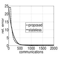
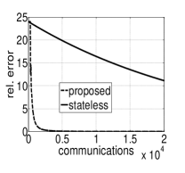
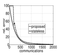
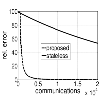
Figure 1: Relative error $(\mathbf{1}^{\top}x^{(k)}-\mathbf{1}^{\top}x^{\star})/(\mathbf{1}^{\top}x^{\star})$ versus per-node communications along iterations for the proposed algorithm (dashed line) and the stateless algorithm in [6] (solid line). Top left: $N=100,\epsilon=1$; top right: $N=100,\epsilon=0.1$; bottom left: $N=400,\epsilon=1$; bottom right: $N=400,\epsilon=0.1$.

VI Conclusion

We introduced a new, neighborhood-based data access model for distributed coded storage allocation where storage nodes are interconnected through a generic network. A user accesses a randomly chosen storage node, and attempts a recovery based on the storage available in the neighborhood set of the accessed node. We formulate the problem of optimally allocating the coded storage such that the overall storage is minimized while probability one recovery is guaranteed. We show that the problem reduces to solving the fractional dominating set problem over the storage node network. Next, we address the problem of designing an efficient fully distributed algorithm to solve the coded storage allocation problem. While existing work did not focus on Lagrangian dual methods, we apply and modify the dual proximal center method. We establish complexity of the method in terms of the desired accuracy and the underlying network and demonstrate its efficiency by simulations.

References

- [1] D. Leong, A. G. Dimakis, and T. Ho, “Distributed storage allocation problems,” in NetCod 2009, Workshop on Network Coding, Theory, and Applications, Lausanne, Switzerland, June 2009, pp. 86–91.
- [2] ——, “Distributed storage allocations,” IEEE Trans. Info. Theory, vol. 58, no. 7, pp. 4733–4752, July 2012.
- [3] F. Kuhn and R. Wattenhofer, “Constant-time distributed dominating set approximation,” Distributed Computing, 2003, DOi: 10.1145/872035.872040.
- [4] M. Luby and N. Nisan, “A parallel approximation algorithm for positive linear programming,” in 25th Annual ACM Symposium on Theory of Computing, San Diego, CA, May 1993, pp. 448–457.
- [5] Y. Bartal, J. Byers, and D. Raz, “Global optimization using local information with applications to flow control,” in 38th Annual Symposium on Foundations of Computer Science, Miami Beach, FL, Oct. 1997, pp. 303–312.
- [6] B. Awerbuch and R. Khandekar, “Stateless distributed gradient descent for positive linear programs,” SIAM J. Comput., vol. 38, no. 6, pp. 2468 –2486, 2009.
- [7] N. E. Young, “Sequential and parallel algorithms for mixed packing and covering,” in 42th Annual Symposium on Foundations of Computer Science, Oct. 2001, pp. 538–546.
- [8] I. Necoara and J. A. Suykens, “Application of a smoothing technique to decomposition in convex optimization,” IEEE Trans. Autom. Contr., vol. 53, no. 11, pp. 2674–2679, Dec. 2008.
- [9] D. Bienstock and G. Iyengar, “Faster approximation algorithms for packing and covering problems,” 2004, available at: http://www.columbia.edu/ dano/papers/tr-2004-09.pdf.
- [10] N. Garg and J. Konemann, “Faster and simpler algorithms for multicommodity flow and other fractional packing problems,” in 39th Annual Symposium on Foundations of Computer Science, Palo Alto, CA, Nov. 1998, pp. 300–309.
- [11] I. Necoara and V. Nedelcu, “Rate analysis of inexact dual first-order methods: Application to dual decomposition,” IEEE Trans. Autom. Contr., vol. 59, no. 5, pp. 123–1243, May 2014.
- [12] E. Cohen and S. Shenker, “Replication strategies in unstructured peer-to-peer networks,” in SIGCOMM 2002, ACM conference on applications, technologies, architectures, and protocols for computer communications, Oct. 2002, pp. 177–190.