Sweeping effect and Taylor’s hypothesis via correlation function

Abstract

We performed high-resolution numerical simulations of hydrodynamic turbulence with and without mean velocity ($U_{0}=0,10$), and demonstrate the sweeping effect. For $U_{0}=0$, the velocity correlation function, $C({\bf k},\tau)$ decays with time due to eddy viscosity, but it also shows fluctuations due to the sweeping effect. For $U_{0}=10$, $C({\bf k},\tau)$ exhibits damped oscillations with the frequency of $U_{0}k$ and decay time scale corresponding to the $U_{0}=0$ case. A closer examination of $\Im[C({\bf k},\tau)]$ also demonstrates sweeping effect for $U_{0}=10$. We also demonstrate that the frequency spectra of the velocity fields measured by real-space probes are respectively $f^{-2}$ and $f^{-5/3}$ for $U_{0}=0$ and 10; these spectra are related to the Lagrangian and Eulerian space-time correlations.

1 Introduction

The incompressible Navier–Stokes equation of a flow that is moving with a mean velocity of ${\mathbf{U}}_{0}$ is

$$\partial_{t}u_{i}+({\mathbf{U}}_{0}\cdot\nabla)u_{i}+\partial_{j}(u_{j}u_{i}) = -\partial_{i}p+\nu\partial^{2}u_{i}+f_{i},$$ (1)

$$\partial_{i}u_{i} = 0,$$ (2)

where ${\bf u}$ is the velocity fluctuation with a zero mean, ${\bf f}$ is the external force, $p$ is the pressure, and $\nu$ is the kinematic viscosity. One of the most important principles of classical physics is Galilean invariance, according to which laws of physics are the same in all inertial frames (frames moving with constant velocities with relative to each other). Naturally, the Navier–Stokes equation, which is Newton’s laws for fluid flows, exhibits this symmetry (Lesieur, 2012; Frisch, 1995; Davidson, 2015; McComb, 1990, 2014). As a consequence of this symmetry, the flow properties of the fluid in the laboratory reference frame (in which the fluid moves with a mean velocity of ${\mathbf{U}}_{0}$) and in the co-moving reference frame (${\mathbf{U}}_{0}=0$) are the same

The velocity field of a turbulent flow is random, hence it is typically characterised by its correlations. There have been several major advances in the understanding the correlations in homogeneous and isotropic turbulence, most notably by Kolmogorov (Kolmogorov, 1941b, a) who showed that in the inertial range, the velocity correlation $C({\bf k})=K_{\mathrm{Ko}}\Pi^{2/3}k^{-5/3}/(4\pi k^{2})$, where $\Pi$ is the energy flux, and $K_{\mathrm{Ko}}$ is the Kolmogorov constant. The corresponding one-dimensional energy spectrum is $E(k)=K_{\mathrm{Ko}}\Pi^{2/3}k^{-5/3}$.

Kraichnan (1964) argued that in the presence of random ${\mathbf{U}}_{0}$, Eulerian field theory does not yield Kolmogorov’s spectrum. In particular, Kraichnan (1964) considered a fluid flow with a random mean velocity field that is constant in space and time but has a Gaussian and isotropic distribution over an ensemble of realisations. Then he employed direct interaction approximation (DIA) to close the hierarchy of equations and showed that $E(k)\sim(\Pi U_{\mathrm{0}})^{1/2}k^{-3/2}$, where $U_{\mathrm{0}}$ is the rms value of the mean velocity. Kraichnan (1964) argued that the above deviation of the energy spectrum from the experimentally observed Kolmogorov’s $k^{-5/3}$ energy spectrum is due to the sweeping effect according to which small-scale fluid structures are advected by the large energy-containing eddies. Due to the above observations, Kraichnan emphasised that the Eulerian formalism is inadequate for obtaining Kolmogorov’s spectrum for a fully developed fluid turbulence. Later, he developed Lagrangian field theory of hydrodynamic turbulence that is consistent with the Kolmogorov’s 5/3 theory of turbulence  (see Kraichnan, 1965, and other related papers). The above framework is called random Galilean invariance.

A related phenomenon is Taylor’s hypothesis of frozen turbulence. Taylor (1938) proposed that the velocity measurement at a point in a fully-developed turbulent flow moving with a constant velocity ${\bf U}_{0}$ (e.g. in a wind tunnel) can be used to study the velocity correlations. This is because the mean flow advects the frozen-in fluctuations, and the stationary probe in the fluid measures the fluctuations along a line. Here, the frequency spectrum of the measured time series is expected to show $\omega^{-5/3}$, where $\omega$ is the angular frequency. This proposal, Taylor’s frozen-in turbulence hypothesis, has been used in many experiments to ascertain Kolmogorov’s spectrum.

In this paper, we investigate the sweeping effect as well as Taylor’s hypothesis using numerical simulations. Using numerical data, we compute the normalised correlation function $R(\mathbf{k},\tau)$, defined as

$$R(\mathbf{k},\tau)=\frac{C(\mathbf{k},\tau)}{C(\mathbf{k},0)}=\frac{\langle\mathbf{u}(\mathbf{k},t)\cdot\mathbf{u}^{*}(\mathbf{k},t+\tau)\rangle}{\langle|\mathbf{u}(\mathbf{k},t)|^{2}\rangle},$$ (3)

where $\mathbf{u}(\mathbf{k},t)$ is the Fourier transform of the velocity field $\mathbf{u}(\mathbf{x},t)$. This measure was earlier proposed by  Sanada & Shanmugasundaram (1992). For $U_{0}=0$, theoretical calculations (Yakhot & Orszag, 1986; McComb, 1990) predict that

$$R(\mathbf{k},\tau)=\exp(-\tau/\tau_{c}(k)),$$ (4)

where $\tau_{c}$ is decay time of an eddy of size $1/k$. The decay time based on local velocity is

$$\tau_{c}(k)\approx\frac{1}{ku_{k}}\sim\Pi^{-1/3}k^{-2/3},$$ (5)

but the decay time based on sweeping by random mean velocity (Kraichnan, 1964) is

$$\tau_{c}(k)\approx\frac{1}{kU_{0}}\sim(U_{0}k)^{-1}.$$ (6)

Sanada & Shanmugasundaram (1992) performed numerical spectral simulations on $256^{3}$ grid resolution and computed $\tau_{c}(k)$. They observed that $\tau_{c}$ is closer to $k^{-1}$ than $k^{-2/3}$, thus arguing in favour of sweeping effect proposed by Kraichnan (1964).

In this paper, we compute $R(\mathbf{k},\tau)$ using numerical simulations and find this to be a complex number whose phase evolution can be related to the advection by random velocity field. We model

$$R(\mathbf{k},\tau)=\exp(-\tau/\tau_{c}(k))\exp(i\tilde{\bf U}_{0}\cdot{\bf k}\tau),$$ (7)

where $\tilde{\bf U}_{0}$ is the random mean velocity. Thus we argue that the effect of the random mean velocity appears in the phase of $R(\mathbf{k},\tau)$, rather than on the absolute value of $R(\mathbf{k},\tau)$ as argued by Sanada & Shanmugasundaram (1992). Using this approach, we validate Kraichnan’s random Galilean invariance.

For finite $U_{0}$ and $U_{0}\gg\tilde{U}_{0}$, we compute $R(\mathbf{k},\tau)$ and observe that

$$R(\mathbf{k},\tau)\sim\exp(-\tau/\tau_{c})\exp(i{\bf U}_{0}\cdot{\bf k}\tau+i\tilde{\bf U}_{0}\cdot{\bf k}\tau).$$ (8)

Thus, an eddy is advected by the mean flow as well as by random mean velocity. For this case, the frequency spectrum of the velocity probe in real space varies as $\omega^{-5/3}$, thus verifying Taylor’s frozen-in turbulence hypothesis (Taylor, 1938). When $U_{0}=0$, the corresponding frequency spectrum is $\omega^{-2}$. We contrast these two cases using correlation function.

In the next section, we briefly describe the sweeping effect and demonstrate its signature using numerical simulation. In §3, we show that the frequency spectrum $E(f)\sim f^{-2}$ for turbulent flow in the absence of a constant mean velocity field $U_{0}$, where $f=\omega/2\pi$. In §4, we discuss Taylor’s frozen-in turbulence hypothesis and show $E(f)\sim f^{-5/3}$ for $U_{0}\gg\tilde{U}_{0}$. In §5, we revisit the elliptic approximation (He et al., 2010; He, 2011; He et al., 2016) in terms of correlation function discussed in §4. We conclude in §6.

2 Sweeping effect and its numerical verification

Here we briefly describe the sweeping effect, first proposed by Kraichnan (1964). Kraichnan assumed that the velocity fluctuation of Navier–Stokes equation is advected by the mean flow, ${\bf U}_{0}$, and random large-scale flow, $\tilde{\bf U}_{0}$. Hence, the temporal evolution of fluctuating Fourier mode ${\bf u}({\bf k})$ is given by

$$\frac{\partial{\bf u}({\bf k})}{\partial t}=-i[{\bf k}\cdot({\bf U}_{0}+\tilde{\bf U}_{0})]{\bf u}({\bf k}).$$ (9)

Kraichnan assumed that $\tilde{\bf U}_{0}$ is spatially varying but is constant in time. Under the assumption of Gaussian distribution for $\tilde{\bf U}_{0}$, Kraichnan (1964) (also see Wilczek & Narita, 2012) showed that

$$R({\bf k},\tau) = \exp[-i{\bf k}\cdot{\bf U}_{0}\tau]\langle\exp[-i{\bf k}\cdot\tilde{\bf U}_{0}\tau]\rangle$$ (10)

$$= \exp[-i{\bf k}\cdot{\bf U}_{0}\tau-\frac{\langle\tilde{U}_{0}^{2}\rangle k^{2}\tau^{2}}{6}].$$ (11)

When we compare the above equation with Eq. (7), we observe that Kraichnan’s derivation does take into account the damping factor $\exp(-\tau/\tau_{c})$.

In the following discussion, using numerical data, we will compute $R({\bf k},\tau)$ that provides signatures of the sweeping effect. Since our analysis is based on the Eulerian framework, it is necessary to review the relevant results of Eulerian field theory that has been employed to analyse the turbulent velocity field. Kraichnan (1959) employed direct interaction approximation (DIA), while Yakhot & Orszag (1986), McComb and coworkers (McComb, 1990), DeDominicis & Martin (1979), Zhou (2010) employed renormalisation group analysis in the Eulerian field-theoretic framework. This is an exhaustive field, and it has been reviewed by McComb (1990, 2014) and Zhou (2010). Also, see Appendix A. For the following discussion, it suffices to remark that the dressed Green’s function for $U_{0}=0$ in the turbulent regime is

$$G({\bf k},\omega)=\frac{1}{-i\omega+\nu(k)k^{2}},$$ (12)

where

$$\nu(k)=\nu_{*}\sqrt{K_{\mathrm{Ko}}}\epsilon^{1/3}k^{-4/3}$$ (13)

is the turbulent viscosity. Here $\nu_{*}$ is a constant whose value is approximately $0.38$ (McComb, 1990) (also see Appendix A). Transformation of the above function to the temporal space yields

$$G({\bf k},\tau)=\theta(\tau)\exp{[-\nu(k)k^{2}\tau)]},$$ (14)

where $\theta(\tau)$ is the step function. The normalised correlation function $R({\bf k},\tau)$ (defined in Eq. (3)) too is time dependent, and it is assumed to have the same relaxation time as the Green’s function, i.e.,

$$R({\bf k},\tau)=\theta(\tau)\exp{[-\nu(k)k^{2}\tau]}.$$ (15)

The above equations indicate that relaxation time scale for the correlation and Green’s functions are

$$\tau_{c}=\frac{1}{\nu(k)k^{2}}\sim\frac{1}{\epsilon^{1/3}k^{2/3}},$$ (16)

where $\nu(k)$ is given by Eq. (13). This is a generalisation of fluctuation dissipation theorem (McComb, 1990). Using the numerically computed $C({\bf k},\tau)$, we estimate the relaxation time and compare it with the predictions of Eulerian field theory.

We perform numerical simulation of Navier–Stokes equation in the turbulent regime for the mean velocity $\mathbf{U}_{0}=0$. We employ pseudospectral code Tarang (Verma et al., 2013) to simulate the flow on a $512^{3}$ grid with random forcing. We use the fourth-order Runge Kutta (RK4) scheme for time stepping, 2/3 rule for dealiasing, and CFL condition for computing $\Delta t$. The Reynolds number of the runs are $u_{\mathrm{rms}}L/\nu=5.7\times 10^{3}$, where $u_{\mathrm{rms}}$ is the rms value of the velocity fluctuations.

We evolve the flow with $U_{0}=0$ till a steady state is reached. At this point, we fork two simulations with ${\mathbf{U}}_{0}=0$ and ${\mathbf{U}}_{0}=10\hat{z}$, and run it for one eddy turnover time. In Fig. 1(a,b) we illustrate velocity profiles of the flows for $U_{0}=0$ and 10 at $t=0.2$. The flow profiles are identical except that the flow for ${\mathbf{U}}_{0}=10\hat{z}$ is shifted vertically by $10\times 0.2=2$ units, as expected. For $U_{0}=0$ and 10, the temporal evolution of the fluctuating energy, as well as the energy spectra, are identical, as illustrated in Fig. 2.

Figure 1: A density plot of the magnitude of the vorticity $|\boldsymbol{\omega}|$ at $t=0.2$ for (a) $\mathbf{U}_{0}=0$ and (b) $\mathbf{U}_{0}=10\hat{z}$. The flow structures in the boxed zone of (b) are shifted by $\Delta z=U_{0}t=10\times 0.2=2$ units compared to (a), thus verifying Galilean invariance of the fluid equation.

These observations on the flow evolution and energy spectra are on expected lines and they illustrate that the Navier–Stokes equation is Galilean invariant. These results, however, are based on equal-time correlations; the subtleties however surface when we study the temporal correlation of the velocity modes.

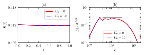
Figure 2: For $U_{0}=0$ and $U_{0}=10$, the plots of (a) total energy of the velocity fluctuation, $u^{2}/2$, vs. $t$ and (b) the normalized kinetic energy spectrum $E(k)k^{5/3}$ vs. $k$. The plots show that $E(t)$ and $E(k)$ are identical for $U_{0}=0,10$, thus verifying Galilean invariance of the fluid equation.

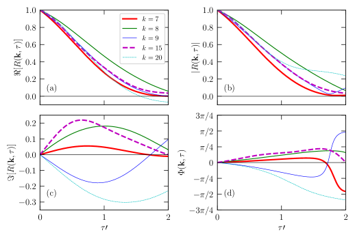
Figure 3: For $\mathbf{U}_{0}=0$ and $k=7,8,9,15,20$ (inertial range wavenumbers), plots of the normalised correlation function $R(\mathbf{k},\tau)$ vs. $\tau^{\prime}=\tau/\tau_{c}$: (a) $\Re[R(\mathbf{k},\tau)]$, (b) $|R(\mathbf{k},\tau)|$, (c) $\Im[R(\mathbf{k},\tau)]$, and (d) $\Phi(\mathbf{k},\tau)$. The real part and the absolute value decay exponentially in time as Eq. (7), while the oscillating imaginary part and monotonic increase of the $\Phi(\mathbf{k},\tau)$ with time demonstrate the sweeping effect.

Using the numerical data, we compute the normalised correlation function $R(\mathbf{k},\tau)$ of Eq. (3), and in Fig. 3 we plot its real and imaginary parts, $\Re[R(\mathbf{k},\tau)]$ and $\Im[R(\mathbf{k},\tau)]$, as well as its magnitude, $|R(\mathbf{k},\tau)|$, and phase

$$\Phi(k,\tau)=\tan^{-1}\frac{\Im[R(\mathbf{k},\tau)]}{\Re[R(\mathbf{k},\tau)]s}$$ (17)

for $k=7,8,9,15$ and 20, which lie in the inertial range. The plot of Fig. 3(a,b) show that $\Re[R(\mathbf{k},\tau)]$ and $|R(\mathbf{k},\tau)|$ decay exponentially with time, consistent with Eq. (7). In Fig. 4, we plot $\tau_{c}^{-1}$ vs. $k$, where $\tau_{c}$ is obtained from the slope of semi-logy plot $|R(\mathbf{k},\tau)|$ vs. $\tau$. A regression analysis yield $\tau_{c}\sim k^{-0.63\pm 0.31}$, which has significant error bar due to a limited range of data. This is due to the relatively narrow inertial range of our $512^{3}$ grid simulations. However, the slope of 0.63 is closer to the exponent of 2/3 than 1, which is contrary to the results of Sanada & Shanmugasundaram (1992). This result indicates that the decay of $R(\mathbf{k},\tau)$ is described by Eq. (15). In the following discussion, we show that $R(\mathbf{k},\tau)$ is a complex number, and its phase contains information about the sweeping effect.

In Figs. 3(c,d) we plot $\Im[R(\mathbf{k},\tau)]$ and the phase $\Phi({\mathbf{k}},\tau)$ of $R(\mathbf{k},\tau)$. The nonzero values of $\Im[R(\mathbf{k},\tau)]$ and the phase $\Phi({\mathbf{k}},\tau)$ indicates that we need to add a new component to Eq. (15). The phases for various $k$’s have the following properties:

1. The phase increases linearly with time till $\tau\approx\tau_{c}$, hence $\Phi({\mathbf{k}},\tau)\propto\tau$ till $\tau\approx\tau_{c}$.

2. In Fig. 3(d), the slopes of the $\Phi({\mathbf{k}},\tau)$ for various $k$’s are different, hence $\Phi({\mathbf{k}},\tau)\neq D\tau$ with a constant $D$ for all $k$’s. Therefore, we can easily conclude that the waves are not advected by a constant mean velocity field, say ${\bf U}_{0}$.

3. The absolute values of the slopes increase with $k$. Note that the slopes come with both positive and negative signs.

Given the above properties, we postulate that for $\tau$ up to $\tau_{c}$,

$$\Phi({\mathbf{k}},\tau)\sim{\bf k}\cdot\tilde{\bf U}_{0}({\bf k})\tau\sim ck\tilde{U}_{0}(k)\tau,$$ (18)

where $c$ is a random number taking both positive and negative signs. Hence the normalised correlation function as well as the Green’s function need to be modified to

$$R(\mathbf{k},\tau)=G(\mathbf{k},\tau) = \exp(-\tau/\tau_{c})\exp(-i{\bf k}\cdot\tilde{\bf U}_{0}({\bf k})\tau)$$ (19)

$$\sim \exp(-\tau/\tau_{c})\exp(-ick\tilde{U}_{0}(k)\tau),$$

which is a numerical demonstration of the sweeping effect proposed by Kraichnan (1964). Physically, a wave ${\bf u}({\bf k})$ is being advected by the random mean velocity field, $\tilde{U}_{0}(k)$. The random velocity changes its direction and magnitude in one eddy turnover time. This is the reason why the phases are linear in $\tau$ only up to $\tau\approx\tau_{c}$. The aforementioned wavenumber-dependent mean velocity field is in the similar spirit as the advection of eddies within eddies (Davidson, 2015; Pope, 2000; McComb, 1990).

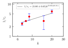
Figure 4: Plot of $\tau_{c}^{-1}$ vs. $k$. We observe that $\tau_{c}^{-1}\sim k^{0.63\pm 0.31}$. The exponent being closer to 2/3 indicates that Eq. (16) is a fair description of the decaying time scale.

Note that the numerically-computed $C({\bf k},\tau)$ is of the form given by Eq. (19), contrary to Eq. (11), as argued by Kraichnan (1964). This is an important deviation from earlier works on sweeping effect. We also remark that it is important to investigate $k$-dependence of $\tilde{U}_{0}(k)$. From scaling arguments, we expect $\tilde{U}_{0}(k)\sim\epsilon^{1/3}k^{-1/3}$. Unfortunately, the present simulation does not have sufficient resolution to test this conjecture. We need to perform a high-resolution simulation that will facilitate a larger range of $k$. If the above conjecture is indeed correct, then the velocity at larger length scale would sweep smaller flow elements embedded within, thus validating the eddies within eddies viewpoint in turbulent flows.

From Eq. (19), we deduce that in ${\bf k}-\omega$ space, the Green’s function is

$$G({\bf k},\omega)=\frac{1}{-i\omega+\nu(k)k^{2}+ick\tilde{U}_{0}(k)}.$$ (20)

Note that the Eulerian field theory does not incorporate the additional term $ick\tilde{U}_{0}(k)$ of the above equation (see Appendix A and McComb, 1990, 2014; McComb & Shanmugasundaram, 1983, 1984; Zhou et al., 1988; Zhou, 2010). This is the reason why Kraichnan (1964) argued that the Eulerian field theory may not be appropriate for the description of hydrodynamic turbulence. To overcome this deficiency, Kraichnan (1965) devised a Lagrangian-based field-theoretic treatment of turbulence. Unfortunately, this topic is beyond the scope of this paper.

Though field-theoretic treatment is not a main theme of the paper, in Appendix A, we discuss this topic very briefly. In the Eulerian treatment of hydrodynamic turbulence, the Green’s function is taken to be of the form of Eq. (12). The perturbative computation shows that the renormalized viscosity is independent of the mean velocity field ${\bf U}_{0}$, which may tempt us to believe that the Eulerian framework respects Galilean invariance. However, as discussed in this section, a more realistic Green’s function consistent with the sweeping effect is of the form given by Eq. (20). Unfortunately, incorporation of this Green’s function makes the perturbative approach quite untenable, consistent with the arguments of Kraichnan (1964) in which he claims nonsuitability of Eulerian field theory for the field-theoretic treatment of turbulence.

In the next section we will describe the frequency spectrum of turbulent flows with $U_{0}=0$.

3 Frequency spectrum of $f^{-2}$ for turbulent flow

It is interesting to note that for homogeneous and isotropic turbulence, the frequency spectrum $E(\omega)$ of the velocity time series measured by a real space probe is proportional to $\omega^{-2}$. This spectrum can be deduced from the correlation function of Eq. (19) in the following manner. The correlation function $C({\bf r},\tau)=\langle{\bf u(x},t)\cdot{\bf u(x+r},t+\tau)\rangle_{{\bf x},t}$, where $\langle.\rangle_{{\bf x},t}$ represents averaging over ${\bf x}$ and $t$, is

$$C({\bf r},\tau) = \int d{\bf k}C({\bf k},\tau)\exp{(i{\bf k\cdot r})}$$ (21)

$$= \int d{\bf k}C({\bf k})\exp(-\nu(k)k^{2}\tau)\exp(-i{\bf k}\cdot\tilde{\bf U}_{0}({\bf k})\tau)\exp(i{\bf k}\cdot{\bf r}).$$

Averaging the above for random $\tilde{\bf U}_{0}({\bf k})$ yields (Kraichnan, 1964; Wilczek & Narita, 2012)

$$C({\bf r},\tau) = \int d{\bf k}C({\bf k})\exp(-\nu(k)k^{2}\tau)\langle\exp(-ick\tilde{U}_{0}(k)\tau)\rangle\exp(i{\bf k}\cdot{\bf r})$$ (22)

$$= \int d{\bf k}C({\bf k})\exp(-\tau/\tau_{c})\exp(-k^{2}[\tilde{U}_{0}(k)]^{2}\tau^{2})\exp(i{\bf k}\cdot{\bf r}).$$

Here we replace the isotropic and homogeneous $C({\bf k})$ with

$$C({\bf k})=\frac{E(k)}{4\pi k^{2}}=\frac{f_{L}(kL)f_{\eta}(k\eta)K_{\mathrm{Ko}}\epsilon^{2/3}k^{-5/3}}{4\pi k^{2}},$$ (23)

where $\epsilon$ is the energy dissipation rate, same as the energy flux, and

$$f_{L}(kL) = \left(\frac{kL}{[(kL)^{2}+c_{L}]^{1/2}}\right)^{5/3+p_{0}},$$ (24)

$$f_{\eta}(k\eta) = \exp\left[-\beta\left\{[(k\eta)^{4}+c_{\eta}^{4}]^{1/4}-c_{\eta}\right\}\right],$$ (25)

with $c_{L},c_{\eta},p_{0},\beta$ as constants. Here $L$ is the large length scale. Note that, here we use Pope (2000) model of a turbulent flow,

$$E(k)=K_{\mathrm{Ko}}\epsilon^{2/3}k^{-5/3}f_{L}(kL)f_{\eta}(k\eta),$$ (26)

to describe the energy spectrum $E(k)$. We also substitute $\tau_{c}(k)=1/(\nu(k)k^{2})=\epsilon^{-1/3}k^{-2/3}$ and $\tilde{U}_{0}(k)=\epsilon^{1/3}k^{-1/3}$ (as argued in the last section). We ignore the coefficients in front of these quantities for brevity.

Since we are measuring the velocity at a single point, we set ${\bf r}=0$. Hence the temporal correlation of the velocity field at a given point ${\bf x}$ is

$$C({\bf r}=0,\tau) = \int d{\bf k}C({\bf k})\exp(-\nu(k)k^{2}\tau)\exp(-k^{2}[\tilde{U}_{0}(k)]^{2}\tau^{2})$$ (27)

$$= K_{\mathrm{Ko}}\epsilon^{2/3}\int dkk^{-5/3}f_{L}(kL)f_{\eta}(k\eta)\exp(-\epsilon^{1/3}k^{2/3}\tau)\times$$

$$\exp(-\epsilon^{2/3}k^{4/3}\tau^{2}).$$

Using $\tau(k)\sim 1/(ku_{k})\sim\epsilon^{-1/3}k^{-2/3}$, we make a change of variable:

$$k=\tilde{k}\epsilon^{-1/2}\tau^{-3/2},$$ (28)

that yields

$$C(\tau) = K_{\mathrm{Ko}}\epsilon\tau\int d{\tilde{k}}\tilde{k}^{-5/3}f_{L}(\tilde{k}(L/U\tau)^{3/2})f_{\eta}(\tilde{k}(\tau_{d}/\tau)^{3/2})\exp(-\tilde{k}^{2/3}-\tilde{k}^{4/3}),$$ (29)

where $U$ is the large-scale velocity, and $\tau_{d}$ is the dissipative time scale. We focus on $\tau$ the inertial range, hence $L/U\tau\gg 1$ and $\tau_{d}/\tau\ll 1$. Therefore, from Eqs. (24), (25), $f_{L}(\tilde{k}(L/U\tau)^{3/2})\approx 1$ and $f_{\eta}(\tilde{k}(\tau_{d}/\tau)^{3/2})\approx 1$ . Therefore,

$$C(\tau)=K_{\mathrm{Ko}}\epsilon\tau\int d{\tilde{k}}\tilde{k}^{-5/3}\exp(-\tilde{k}^{2/3}-\tilde{k}^{4/3})=AK_{\mathrm{Ko}}\epsilon\tau,$$ (30)

where $A$ is the value of the integral of Eq. (29). The Fourier transform of $C(\tau)$ yields the frequency spectrum, which is

$$C(\omega) = \int C(\tau)\exp(i\omega\tau)d\tau=AK_{\mathrm{Ko}}\epsilon\int\tau\exp(i\omega\tau)d\tau\sim\epsilon\omega^{-2}\sim\epsilon f^{-2},$$ (31)

where $f=\omega/(2\pi)$. Thus we show that the frequency spectrum $E(f)\sim f^{-2}$.

To compute the frequency spectrum $E(f)$ from the time series of the velocity field, we placed $50$ real space probes at random locations in the cubical box. We record the three components of the velocity field at all the real space probes. We run our simulation for single eddy turnover time with a constant $\Delta t=3\times 10^{-5}$, which helps us compute the Fourier transform of the real space data using equispaced FFT. Note that for $\Delta t=3\times 10^{-5}$, the Courant number is less than unity; hence our simulation is well resolved in time. We record the velocity fields at every $33$ steps; thus we have $10^{3}$ data points. Then we perform Fourier transform of the velocity components $u_{i}(t)$ ($i=x,y,z$) and compute the frequency spectrum $E(f)$ using following formula

$$E(f)=\frac{1}{2}\left(|\hat{u}_{x}(f)|^{2}+|\hat{u}_{y}(f)|^{2}+|\hat{u}_{z}(f)|^{2}\right).$$ (32)

Figure 5 exhibits the averaged frequency spectrum that exhibits $f^{-2}$ scaling, consistent with Eq. (31). Earlier, Landau & Lifshitz (1987) had derived the aforementioned power law using dimensional analysis. We will revisit their arguments in the next section.

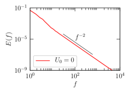
Figure 5: For $U_{0}=0$, plot of the frequency spectrum $E(f)$ for the velocity time series measured by a real space probe. The plot is averaged over 50 real space probes located at random locations. Here $E(f)\sim f^{-2}$, consistent with the sweeping effect (see Eq. (31)).

In the next section, we will report the numerical results for ${\bf U}_{0}=10\hat{z}$ and show the effects of the mean velocity field on the correlation function, which is related to Taylor’s frozen-in turbulence hypothesis.

4 Taylor’s frozen-in turbulence hypothesis

We compute the correlation function when $U_{0}\neq 0$; this phenomenon is related to Taylor’s frozen-in turbulence hypothesis. In this paper, we present our results for ${\bf U}_{0}=10\hat{z}$.

As described in §2, we performed numerical simulation of incompressible fluid with ${\bf U}_{0}=0$ and ${\bf U}_{0}=10\hat{z}$. Compared to the flow for $U_{0}=0$, the flow profile for ${\bf U}_{0}=10\hat{z}$ is shifted upward as shown in Fig. 1, and the energy spectrum and flux are the same as for $U_{0}=0$ and 10. The correlation function for ${\bf U}_{0}=10\hat{z}$, however, exhibits features very different from that for $U_{0}=0$; this phenomenon is related to Taylor’s hypothesis.

We compute $R(k,\tau)$ of Eq. (3) using the numerical data. We choose ${\bf k}=(0,0,10)$. In Fig. 6, we plot the real and imaginary parts of the correlation $R(\mathbf{k},\tau)$, as well as its magnitude and phase. As shown in the figure, $|R(\mathbf{k},\tau)|$ is approximately same for $U_{0}=0$ and 10. However, both the real and imaginary parts of $R(\mathbf{k},\tau)$ exhibit damped oscillations with a frequency of $\omega=k_{z}U_{0}$ and a decay time scale of $1/(\nu(k)k^{2})$. This is evident from the envelop of $\Re[R(\mathbf{k},\tau)]$ that matches with $\Re[R(\mathbf{k},\tau)]$ for $U_{0}=0$. Hence, we may naively expect that

$$R(\mathbf{k},\tau)=G(\mathbf{k},\tau)=\exp(-\tau/\tau_{c})\exp(i{\bf U}_{0}\cdot{\bf k}\tau).$$ (33)

However, there are some signatures of random sweeping effect for $U_{0}=10$ as well. In Fig. 6, we plot the phase $\Phi$ of $R(\mathbf{k},\tau)$, which is quite close to $U_{0}k\tau$. However, $\Phi-U_{0}k\tau$ is nonzero, which is evident from its magnified plot in Fig. 6(d). This deviation is due to the random sweeping effect by random mean field $\tilde{U}_{0}$. Thus, the small-scale fluctuations are swept by ${\bf U}_{0}=10\hat{z}$ and by large-scale random velocity $\tilde{U}_{0}(k)$. The effects of $\tilde{U}_{0}(k)$ for ${\bf U}_{0}=10\hat{z}$ and ${U}_{0}=0$ are expected to be the same, since the velocity fluctuations are the same in both the flows. Therefore, the Green’s function and the normalised correlation function for ${\bf U}_{0}=10\hat{z}$ can be written as

$$R(\mathbf{k},\tau)=G(\mathbf{k},\tau)=\exp(-\tau/\tau_{c})\exp(-i{\bf U}_{0}\cdot{\bf k}\tau-ck\tilde{U}_{0}(k)\tau),$$ (34)

and

$$G({\bf k},\omega)=\frac{1}{-i\omega+\nu(k)k^{2}+i{\bf U}_{0}\cdot{\bf k}+ick\tilde{U}_{0}(k)}.$$ (35)

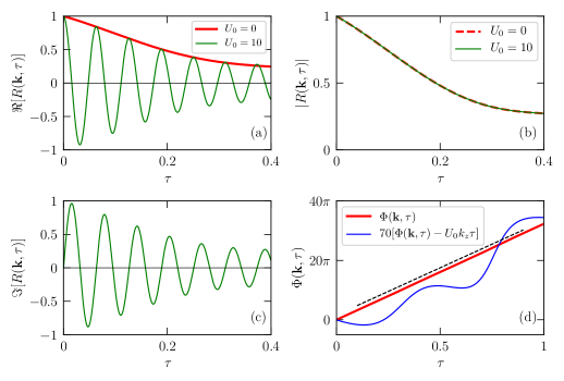
Figure 6: For $\mathbf{U}_{0}=10$ and $\mathbf{k}=(0,0,10)$ in the inertial range), plots of the normalised correlation function $R(\mathbf{k},\tau)$ vs. $\tau$: (a) $\Re[R(\mathbf{k},\tau)]$, (b) $|R(\mathbf{k},\tau)|$, (c) $\Im[R(\mathbf{k},\tau)]$, and (d) $\Phi(\mathbf{k},\tau)$. The real and imaginary parts exhibit damped oscillation with the frequency of $U_{0}k$ and damping time of $1/(\nu(k)k^{2})$. $|R(\mathbf{k},\tau)|$ for $U_{0}=0,10$ are identical, thus showing that the decay time scales for the two cases are the same; also, $|R(\mathbf{k},\tau)|$ provides envelop to the real part. The phase of $R(\mathbf{k},\tau)$ varies as $\Phi({\bf k},\tau)=U_{0}k_{z}\tau+\delta$, where $\delta$ arises due to the sweeping by the random large-scale flow structures. The dashed black and blue lines represent $U_{0}k_{z}\tau$ and $70\delta$ (amplified by a factor for visualisation) respectively.

Now let us discuss Taylor’s frozen-in turbulence hypothesis, according to which the frequency spectrum of the real-space velocity time series $E(f)\sim f^{-5/3}$. This conclusion can be easily derived using the correlation function of Eq. (34). Following the same set of mathematical steps as in the earlier section on the correlation function of Eq. (34), we obtain

$$C({\bf r},\tau) = \int d{\bf k}C({\bf k})\exp(-\nu(k)k^{2}\tau-i{\bf U_{0}\cdot k}\tau)\exp(-i{\bf k}\cdot\tilde{\bf U}_{0}({\bf k})\tau)\exp(i{\bf k}\cdot{\bf r}).$$ (36)

We time average $\tilde{U}_{0}$ over random ensemble that yields

$$C({\bf r},\tau) = \int d{\bf k}C({\bf k})\exp(-\nu(k)k^{2}\tau-i{\bf U_{0}\cdot k}\tau)\langle\exp(-ick\tilde{U}_{0}(k)\tau)\rangle\exp(i{\bf k}\cdot{\bf r})$$ (37)

$$= \int d{\bf k}C({\bf k})\exp(-\tau/\tau_{c}-i{\bf U_{0}\cdot k}\tau)\exp(-k^{2}[\tilde{U}_{0}(k)]^{2}\tau^{2})\exp(i{\bf k}\cdot{\bf r}).$$

Since we are measuring the velocity at a single point, we set ${\bf r}=0$. We also replace $C({\bf k})$ of the above equation with that of Eq. (23) that yields

$$C(\tau) = K_{\mathrm{Ko}}\epsilon^{2/3}\int dkk^{-5/3}f_{L}(kL)f_{\eta}(k\eta)\exp(-i{\bf U_{0}\cdot k}\tau)\times$$ (38)

$$\exp(-\epsilon^{1/3}k^{2/3}\tau)\exp(-\epsilon^{2/3}k^{4/3}\tau^{2}).$$

For the integration, we choose the $z$ axis along the direction of ${\bf U}_{0}$. Since $\tau\sim 1/(U_{0}k)$ is the dominant time scale, we make a change of variable:

$$\tilde{k}=U_{0}k\tau$$ (39)

that yields

$$C(\tau) = K_{\mathrm{Ko}}(\epsilon U_{0}\tau)^{2/3}\int d{\tilde{k}}\tilde{k}^{-5/3}f_{L}(\tilde{k}(L/U_{0}\tau))f_{\eta}(\tilde{k}(\eta/U_{0}\tau)\frac{\sin(U_{0}k\tau)}{U_{0}k\tau}\times$$ (40)

$$\exp[-\tilde{k}^{2/3}(U/U_{0})^{2/3}(\tau/T)^{1/3}-\tilde{k}^{4/3}(U/U_{0})^{4/3}(\tau/T)^{2/3}].$$

We focus on $\tau$ in the inertial range, hence $L/U_{0}\tau\gg 1$ and $\eta/U_{0}\tau\ll 1$, consequently, $f_{L}(\tilde{k}(L/U_{0}\tau))\approx 1$, and $f_{\eta}(\tilde{k}(\eta/U_{0}\tau)\approx 1$. Therefore,

$$C(\tau) = K_{\mathrm{Ko}}(\epsilon U_{0}\tau)^{2/3}\int d{\tilde{k}}\tilde{k}^{-5/3}\frac{\sin\tilde{k}}{\tilde{k}}\exp[-\tilde{k}^{2/3}(U/U_{0})^{2/3}(\tau/T)^{1/3}-\tilde{k}^{4/3}(U/U_{0})^{4/3}(\tau/T)^{2/3}]$$ (41)

$$= B\alpha K_{\mathrm{Ko}}(\epsilon U_{0}\tau)^{2/3},$$

where $B$ is the value of the integral. The Fourier transform of the above $C(\tau)$ yields the frequency spectrum

$$C(\omega) = \int C(\tau)\exp(i\omega\tau)d\tau=\int BK_{\mathrm{Ko}}(\epsilon U_{0}\tau)^{2/3}\exp(i\omega\tau)d\tau$$ (42)

$$\sim (\epsilon U_{0})^{2/3}\omega^{-5/3}\sim(\epsilon U_{0})^{2/3}f^{-5/3}.$$

This is the Taylor’s frozen-in turbulence hypothesis (Taylor, 1938), according to which the frequency spectrum of the velocity field measured by a real space probe also yields Kolmogorov’s $-5/3$ spectrum. This is very useful hypothesis because to determine $E(k)$, we do not need to measure the velocity field at all physical locations by expensive experimental setups. Researchers have exploited the above hypothesis to measure turbulence spectrum in many fluid and plasma experiments, for example in wind tunnels, and measurement of solar wind turbulence using extraterrestrial spacecrafts.

We could also argue the above frequency spectrum using scaling arguments (Landau & Lifshitz, 1987). From the definition of Green’s function (35), we obtain the dominant $\omega=\mathbf{U}_{0}\cdot\mathbf{k}+k\tilde{U}_{0}(k)-i\nu(k)k^{2}$. When $\mathbf{U}_{0}\cdot\mathbf{k}\gg\nu(k)k^{2}$ and $\mathbf{U}_{0}\cdot\mathbf{k}\gg k\tilde{U}_{0}(k)$, we obtain $\omega=U_{0}k_{z}$. Therefore, using $E(k)=K_{\mathrm{Ko}}\Pi^{2/3}k^{-5/3}$, we obtain

$$E(\omega) = E(k)\frac{dk}{d\omega}\sim K_{\mathrm{Ko}}\Pi^{2/3}(\omega/U_{0})^{-5/3}(1/U_{0})$$ (43)

$$\sim K_{\mathrm{Ko}}(U_{0}\Pi)^{2/3}\omega^{-5/3},$$

consistent with the principle of Taylor’s frozen-in turbulence hypothesis. Here we have replaced $k$ by $k_{z}$. On the contrary, when $\mathbf{U}_{0}\cdot\mathbf{k}\ll\nu(k)k^{2}$ (for zero or small $U_{0}$), we obtain

$$\omega\approx\nu(k)k^{2}=\nu_{*}\sqrt{K_{\mathrm{Ko}}}\Pi^{1/3}k^{2/3},$$ (44)

and hence, using $E(k)=K_{\mathrm{Ko}}\Pi^{2/3}k^{-5/3}$, we obtain

$$E(\omega) = E(k)\frac{dk}{d\omega}$$ (45)

$$= \frac{K_{\mathrm{Ko}}\Pi^{2/3}k^{-5/3}}{\nu_{*}\sqrt{K_{\mathrm{Ko}}}\Pi^{1/3}(2/3)k^{-1/3}}$$

$$= \frac{3}{2}\nu_{*}(K_{\mathrm{Ko}})^{3/2}\Pi\omega^{-2},$$

as derived by Landau & Lifshitz (1987). Thus, the Green’s function of Eq. (35) helps us deduce both $\omega^{-5/3}$ and $\omega^{-2}$ frequency spectra depending on the strength of ${\bf U}_{0}$. The above discussion also demonstrates that the Eulerian picture picks up both, the sweeping effect and Taylor’s hypothesis. We refer the reader to Tennekes (1975) and He et al. (2016) for Eulerian and Lagrangian time scales, and their connection to $\omega^{-2}$ and $\omega^{-5/3}$ power spectra.

To test Taylor’s frozen-in turbulence hypothesis numerically, we record time series of the velocity field at the real space probes, and then compute their frequency spectrum $E(f)$, same analysis as that of the previous section, but here with ${\bf U}_{0}=10\hat{z}$. Figure 7(a) exhibits $E(k)$ and $E(f)$ in the presence of mean velocity field ${\bf U}_{0}=10\hat{z}$, for which both the spectra follow Kolmogorov’s scaling (see Eq. (43)). Note that in Fig. 7(a) we scaled the frequency spectrum: $f\rightarrow\tilde{f}=f(2\pi)/U_{0}$ and $E(f)\rightarrow\tilde{E}(\tilde{f})=E(f)U_{0}/(2\pi)$. Our result that $\tilde{E}(\tilde{f})\approx E(k)$ illustrates Taylor’s hypothesis in the presence of a mean velocity field.

For $U_{0}\ll u_{L}$ or $U_{0}\ll\epsilon^{1/3}L^{1/3}$, as argued above, Taylor’s frozen-in turbulence hypothesis will not work. Rather, the sweeping effect by local mean velocity would dominate the dynamics, hence we expect $E(f)\sim f^{-2}$. To test this hypothesis, we perform a numerical simulation for ${\bf U}_{0}=0.4\hat{z}$ following the same procedure as that for ${\bf U}_{0}=10\hat{z}$. For ${\bf U}_{0}=0.4\hat{z}$, Fig. 7(b) exhibits the averaged frequency spectra, which exhibit $f^{-2}$ scaling, which is consistent with the above arguments.

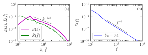
Figure 7: (a) For $U_{0}=10$, plots of the wavenumber spectrum $E(k)$ and the scaled frequency spectrum $E(f)$ for the velocity time series measured by real-space probes. The plot is averaged over 50 real-space probes located at random locations. Here $\tilde{f}=f(2\pi)/U_{0}$ and $\tilde{E}(\tilde{f})=E(f)U_{0}/(2\pi)$. $E(f)\sim f^{-5/3}$, consistent with Taylor’s frozen-in turbulence hypothesis. (b) For $U_{0}=0.4$, $U_{0}\ll\tilde{U}_{0}$, hence $E(f)\sim f^{-2}$, consistent with the sweeping effect. Also see Fig. 5.

In the next section, we describe elliptic approximation that relates space-time correlation to equal-time correlation function.

5 Elliptic approximation

Recently He et al. (2010), He (2011), and He et al. (2016) attempted to combine the sweeping effect with Taylor’s frozen-in turbulence hypothesis. Here we reproduce their arguments using Eq. (36).

We consider fluid flow with a mean velocity of $U_{0}$ along the $z$ axis. We focus on the vertical velocities measured at two points $z$ and $z+r$, but at times $t$ and $t+\tau$ (see Fig. 8 for an illustration). For the same, the space-time correlation derived using Eq. (36) is

$$C(r,\tau) = \int d{\bf k}C({\bf k})\exp(-\nu(k)k^{2}\tau)\exp\left\{[r-i(U_{0}+\tilde{U}_{0z})\tau)]ik_{z}-i\tilde{\bf U}_{0\perp}\cdot{\bf k}_{\perp}\tau\right\}.$$ (46)

Now suppose that

$$r\approx U_{0}\tau\gg\nu(k)k^{2}\tau,$$ (47)

then

$$C(r,\tau)=\int d{\bf k}C({\bf k})\exp\left\{[r-(U_{0}+\tilde{U}_{0z})\tau)]ik_{z}-i\tilde{\bf U}_{0\perp}\cdot{\bf k}_{\perp}\tau\right\}.$$ (48)

We can relate the above correlation function to an equal-time correlation function

$$C({\bf r}_{E},0)=\exp[ir_{Ez}k_{z}+i{\bf r}_{E\perp}\cdot{\bf k}_{\perp}]$$ (49)

with

$$r_{Ez}=[r-(U_{0}+\tilde{U}_{0z})\tau)];~{}~{}{\bf r}_{E\perp}=\tilde{\bf U}_{0\perp}\tau$$ (50)

or

$$r_{E}^{2}=r_{Ez}^{2}+|{\bf r}_{E\perp}|^{2}=(r-U\tau)^{2}+(V\tau)^{2},$$ (51)

where

$$U = U_{0}+\tilde{U}_{0z}$$ (52)

$$V = |\tilde{\bf U}_{0\perp}|.$$ (53)

This is the statement of elliptic approximation (He et al., 2010; He, 2011; He et al., 2016). Our derivation is slightly different from those of He et al. (2010), He (2011), and He et al. (2016).

Thus, the elliptic approximation includes both, the sweeping effect and Taylor’s frozen-in turbulence hypothesis. The velocities $U_{0}$ and $\tilde{U}_{0}$ yield the Eulerian and Lagrangian space-time correlations respectively, and they are related to the sweeping effect and Taylor’s hypothesis respectively. It is easy to see that the conventional Taylor’s hypothesis is applicable when $U_{0}\gg\tilde{U}_{0}$ and it yields $f^{-5/3}$ spectrum, for which the physical interpretation is as follows. The velocity correlation for the velocity measurements at A and B of Fig. 8, $C(r,\tau)=\langle{\bf u}(z,t){\bf u}(z+r,t+\tau)\rangle$, is same as those measured at A and ${\rm B}^{\prime}$ at the same time $t$, $C(r_{E},0)=\langle{\bf u}(z,t){\bf u}(z+r-U_{0}\tau,t)\rangle$. This is because the fluid element at ${\rm B}^{\prime}$ at time $t$ reaches B at time $t+\tau$. Note that Taylor’s frozen-in turbulence hypothesis assumes that $r=0$; for this case, ${\rm B}^{\prime}$ would be at $z-U_{0}\tau$.

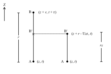
Figure 8: A and B represent respectively the velocity measurements at locations $z$ and $z+r$ and at times $t$ and $t+\tau$. The fluid element at B would be at ${\rm B}^{\prime}$ at time $t$, thus A and ${\rm B}^{\prime}$ would represent equal-time measurements. Note that $r_{E}=r-U_{0}\tau$.

Sreenivasan & Stolovitzky (1996) analysed the velocity fluctuations of the atmospheric data and showed that the conditional expectation of $\Delta u_{r}^{2}$ depends on the local mean velocity field $u_{0}$ for small Reynolds number, but it is independent of $u_{0}$ for large Reynolds number. Here $\Delta u_{r}=u(x+r)-u(x)$, where $u$ and $r$ are respectively the velocity component and the separation distance in the direction $x$. This is due to the dominance of Lagrangian space-time correlation (He et al., 2016). In a related work, Cholemari & Arakeri (2006) proposed a model to relate the spatial and temporal Eulerian two-point correlations in the absence of mean flow. We also remark that He et al. (2010) employed elliptic approximation to Rayleigh-Bénard convection, and related the frequency spectrum of a real-space probe to the energy spectrum, $E(k)$.

6 Discussions and Conclusions

Using numerical simulations, we investigate the sweeping effect and Taylor’s frozen-in turbulence hypothesis, and show consistency between them. We performed numerical simulations with and without mean flow ($U_{0}=10$ and 0 respectively). The velocity fluctuations for the two cases exhibit identical energy spectra and energy fluxes, but the space-time correlations for the two cases are different.

For $U_{0}=0$, we compute the velocity correlation function $C(k,\tau)$ and show that its real part decays with time-scale $1/(\nu(k)k^{2})$, where $\nu(k)$ is the renormalised viscosity. However, the phase of the correlation function shows a linear increase with $\tau$ till approximately one eddy turnover time; this is attributed to the sweeping by random mean velocity of the flow. Thus we demonstrate a clear signature of sweeping effect in hydrodynamic turbulence. Our approach deviates from those of Sanada & Shanmugasundaram (1992) who use absolute of correlation function. Note that the phase of the correlation function extracts the effects of the sweeping effect by random mean velocity.

For $U_{0}=10$, the correlation function exhibits damped oscillations with a frequency of $\omega=U_{0}k$ and decay time scale of $1/(\nu(k)k^{2})$; the decay time scales for $U_{0}=10$ is same as that for $U_{0}=0$. A careful examination of the phase of the correlation function also shows additional variations due to random velocity of the flow.

For the aforementioned two cases, the frequency spectra of the velocity field measured by real-space probes are different. For $U_{0}=0$, $E(f)\sim f^{-2}$, which is related to the Lagrangian space-time correlation, but for $U_{0}=10$, $E(f)\sim f^{-5/3}$, which is the predictions of Taylor’s frozen-in turbulence hypothesis. We demonstrate these spectra from their respective space-time correlation functions. Our analysis shows that Taylor’s hypothesis is applicable when

$$U_{0}k\gg\nu(k)k^{2};~{}~{}~{}U_{0}\gg\tilde{U}_{0},$$ (54)

where $\tilde{U}_{0}$ is random mean velocity, which is responsible for the sweeping effect.

Thus, we provide a systematic demonstration of sweeping effect and Taylor’s frozen-in turbulence hypothesis, and show consistency between the two contrasting phenomena. We demonstrate the above spectra using numerical simulations.

Appendix A Renormalization group analysis in the presence of $\mathbf{U}_{0}$

Hydrodynamic turbulence involves multi scales, hence, renormalization group (RG) formulation is a useful tool to study hydrodynamic turbulence. Some of the leading efforts on the RG formulation of hydrodynamic turbulence are: Yakhot-Orszag perturbative approach (Yakhot & Orszag, 1986), self-consistent approach of McComb (1990) and Zhou (2010), and generating functional formulation of DeDominicis & Martin (1979). See recent review of Zhou (2010) for further discussion. Most of the aforementioned computations are for zero mean flow. In this Appendix we make an extension of McComb’s procedure (McComb, 1990) for $U_{0}\neq 0$.

Navier–Stokes equations describe fluid flows in real space. The corresponding equations in the Fourier space are

$$(-i\omega+i{\mathbf{U}_{0}\cdot\mathbf{k}}+\nu k^{2})u_{i}(\hat{{k}}) = -\frac{i}{2}P_{ijm}(\mathbf{k})\int_{\hat{{p}}+\hat{{q}}=\hat{{k}}}d\hat{{p}}\left[u_{j}(\hat{{p}})u_{m}(\hat{{q}})\right]+f_{i}(\hat{k}),$$ (55)

$$k_{i}u_{i}({\bf k}) = 0,$$ (56)

where

$$P_{ijm}(\mathbf{k})=k_{j}P_{im}(\mathbf{k})+k_{m}P_{ij}(\mathbf{k}),$$ (57)

$$\hat{k}=(\omega,\mathbf{k}),\hat{p}=(\omega^{\prime},\mathbf{p}),\mathrm{and}\,\,\hat{q}=(\omega^{\prime\prime},\mathbf{q}).$$

We compute the renormalized viscosity in the presence of a mean velocity $\mathbf{U}_{0}$. In this renormalization process, the wavenumber range $(k_{N},k_{0})$ is divided logarithmically into $N$ shells. The $n$th shell is $(k_{n},k_{n-1})$ where $k_{n}=h^{n}k_{0}\,\,(h<1)$ and $k_{N}=h^{N}k_{0}$. In the first step, the spectral space is divided in two parts: the shell $(k_{1},k_{0})=k^{>}$, which is to be eliminated, and $(k_{N},k_{1})=k^{<}$, set of modes to be retained. The equation for a Fourier mode $\hat{k}$ belonging to $k^{<}$ is

$$\bigl{[}-i\omega+ i{\mathbf{U}_{0}\cdot\mathbf{k}}+\nu_{(0)}k^{2}\bigr{]}u_{i}^{<}(\hat{k})=-\frac{i}{2}P_{ijm}({\textbf{k}})\int_{\hat{{p}}+\hat{{q}}=\hat{k}}d\hat{p}([u_{j}^{<}(\hat{p})u_{m}^{<}(\hat{q})]$$ (58)

$$+2[u_{j}^{<}(\hat{p})u_{m}^{>}(\hat{q})]+[u_{j}^{>}(\hat{p})u_{m}^{>}(\hat{q})])+f^{<}_{i}(\hat{k}),$$

where $\nu_{(0)}=\nu$. The equation for $u_{i}^{>}(\hat{k})$ modes can be obtained by interchanging $<$ and $>$ in the above equations.

The objective of the renormalization group procedure is to compute the corrections to the viscosity, $\delta\nu_{(0)}$, due to the second and third terms in the RHS of Eq. (58). The steps shown below are same as the i-RG or iterative averaging RG procedure (McComb, 1990, 2014; McComb & Shanmugasundaram, 1983, 1984; Zhou et al., 1988; Zhou, 2010; Verma, 2004).

1. The terms given in the second and third brackets in the right-hand side of Eq. (58) are computed perturbatively. Since we are interested in the statistical properties of the velocity fluctuations, we perform an ensemble average of the system (Yakhot & Orszag, 1986). It is assumed that $\mathbf{u}^{>}(\hat{k})$ have a gaussian distribution with a zero mean, while $\mathbf{u}^{<}(\hat{k})$ is unaffected by the averaging process. Hence,

   $$\left\langle u_{i}^{>}(\hat{k})\right\rangle=0;~{}~{}\left\langle u_{i}^{<}(\hat{k})\right\rangle=u_{i}^{<}(\hat{k}).$$ (59)

   The homogeneity of turbulent fluctuations yields (Batchelor, 1971)

   $$\left\langle u_{i}^{>}(\hat{p})u_{j}^{>}(\hat{q})\right\rangle = P_{ij}(\mathbf{p})C(\hat{p})\delta(\hat{p}+\hat{q}).$$ (60)

   The triple order correlations $\left\langle u_{i}^{>}(\hat{k})u_{j}^{>}(\hat{p})u_{m}^{>}(\hat{q})\right\rangle$ are zero due to the Gaussian nature of the fluctuations. In addition, we neglect the contribution from the triple nonlinearity $\left\langle u^{<}(\hat{k})u_{j}^{<}(\hat{p})u_{m}^{<}(\hat{q})\right\rangle$, as assumed in some of the RG calculations of turbulence (Yakhot & Orszag, 1986; Zhou et al., 1988; McComb, 1990; Zhou, 2010; McComb, 2014). The effects of triple nonlinearity can be included following the scheme proposed by Zhou et al. (1988) and Zhou (2010).

2. To first order, the second bracketed term of Eq. (58) vanishes, but the nonvanishing third bracketed term yields corrections to $\nu_{(0)}$ (McComb, 1990, 2014; McComb & Shanmugasundaram, 1983, 1984; Zhou et al., 1988; Zhou, 2010; Verma, 2004). Consequently, Eq. (58) becomes

   $$\bigl{[}-i\omega +i{\mathbf{U}_{0}\cdot\mathbf{k}}+(\nu_{(0)}(k)+\delta\nu_{(0)}(k))k^{2}\bigr{]}u_{i}^{<}(\hat{k})=$$ (61)

   $$-\frac{i}{2}P_{ijm}({\textbf{k}})\int_{\hat{{p}}+\hat{{q}}=\hat{k}}\frac{d\mathbf{p}d\omega^{\prime}}{(2\pi)^{d+1}}[u_{j}^{<}(\hat{p})u_{m}^{<}(\hat{k}-\hat{p})]+f^{<}_{i}(\hat{k})$$

   with

   $$\delta\nu_{(0)}(\hat{k})k^{2}=\frac{1}{d-1}\int_{\hat{p}+\hat{q}=\hat{k}}^{\Delta}\frac{d\mathbf{p}d\omega^{\prime}}{(2\pi)^{d+1}}[B(k,p,q)G(\hat{q})C(\hat{p})],$$ (62)

   where

   $$B(k,p,q)=kp[(d-3)z+2z^{3}+(d-1)xy]$$ (63)

   with $d$ is the space dimensionality, $x,y,z$ are the direction cosines of ${{\mathbf{k}},{\mathbf{p}},{\mathbf{q}}}$, and the Green’s function $G(\hat{q})$ is defined as

   $$G(\hat{q})=\frac{1}{-i\omega^{\prime\prime}+i{\mathbf{U}_{0}\cdot\mathbf{q}}+\nu_{(0)}(q)q^{2}}.$$ (64)

   It is assumed in the RG calculation of turbulence that the correlation function and the Green’s function have the same frequency dependence, which is a generalization of fluctuation dissipation theorem (McComb, 1990). Hence, the correlation function $C(\hat{p})$ is defined as

   $$C(\hat{p})=\frac{C({\bf p})}{-i\omega^{\prime}+i{\mathbf{U}_{0}\cdot\mathbf{p}}+\nu_{(0)}(p)p^{2}},$$ (65)

   where $C({\bf p})$ is the modal energy spectrum. In §4, we show that the sweeping effect induces an additional term of the form $i{\tilde{\mathbf{U}}_{0}\cdot\mathbf{p}}$ in Green’s function (see Eq. (35)).

3. A substitution of Green’s function and the correlation function in Eq. (62) yields

   $$\delta\nu_{(0)}(\hat{k})k^{2}=\frac{1}{d-1} \int_{\hat{p}+\hat{q}=\hat{k}}\frac{d\mathbf{p}d\omega^{\prime}}{(2\pi)^{d+1}}B(k,p,q)C(\mathbf{p})$$ (66)

   $$\times\frac{1}{[-i\omega^{\prime\prime}+i{\mathbf{U}_{0}\cdot\mathbf{q}}+\nu_{(0)}(q)q^{2}]}$$

   $$\times\frac{1}{[-i\omega^{\prime}+i{\mathbf{U}_{0}\cdot\mathbf{p}}+\nu_{(0)}(p)p^{2}]}.$$

   Using $\omega=\omega^{\prime}+\omega^{\prime\prime}$, we obtain

   $$\delta\nu_{(0)}(\omega,k)k^{2} = \frac{1}{d-1}\int_{\hat{p}+\hat{q}=\hat{k}}\frac{d\mathbf{p}d\omega^{\prime}}{(2\pi)^{d+1}}B(k,p,q)C(\mathbf{p})$$ (67)

   $$\times\frac{1}{\bigl{[}-i\omega+i\omega^{\prime}+i{\mathbf{U}_{0}\cdot\mathbf{q}}+\nu_{(0)}(q)q^{2}\bigr{]}\bigl{[}-i\omega^{\prime}+i{\mathbf{U}_{0}\cdot\mathbf{p}}+\nu_{(0)}(p)p^{2}\bigr{]}}$$

   $$= \frac{1}{d-1}\int_{\bf{p+q=k}}^{\Delta}\frac{d\mathbf{p}}{(2\pi)^{d}}B(k,p,q)C(\mathbf{p})$$

   $$\times\frac{1}{\bigl{[}-i\omega+\nu_{(0)}(p)p^{2}+\nu_{(0)}(q)q^{2}+(i{\mathbf{U}_{0}\cdot\mathbf{p}}+i{\mathbf{U}_{0}\cdot\mathbf{q}})\bigr{]}}$$

   $$= \frac{1}{d-1}\int_{\bf{p+q=k}}^{\Delta}\frac{d\mathbf{p}}{(2\pi)^{d}}B(k,p,q)C(\mathbf{p})$$

   $$\times\frac{1}{\bigr{[}-i(\omega-{\mathbf{U}}_{0}\cdot{\mathbf{k}})+\nu_{(0)}(p)p^{2}+\nu_{(0)}(q)q^{2}\bigr{]}}.$$

   We employ a contour integral to integrate $\omega^{\prime}$ to go from the first step to the second step of Eq. (67). The integration $d\bf p$ is performed over the wavenumber shell $(k_{1},k_{0})$.

4. $\omega-{\mathbf{U}}_{0}\cdot{\mathbf{k}}=\omega_{D}$ is the Doppler-shifted frequency in the moving frame, where the frequency of the signal is reduced. It is analogous to the reduction of frequency of the sound wave in a moving train when the train moves away from the source. For $U_{0}=0$, it is customary to assume that $\omega\rightarrow 0$ since we focus on dynamics at large time scales (Yakhot & Orszag, 1986; Zhou et al., 1988; McComb, 1990; Zhou, 2010; McComb, 2014). The corresponding assumption is to set $\omega_{D}\rightarrow 0$ because $\omega_{D}$ is the effective frequency in the moving frame in which ${\bf U}_{0}=0$. The approximation $\omega\rightarrow{\mathbf{U}}_{0}$ essentially takes away the effect of Galilean transformation and yields inherent turbulence properties. Note that in Taylor’s frozen-in turbulence hypothesis, $\omega={\bf U_{0}\cdot k}$ that yields $\omega_{D}=0$ (see §4). Therefore,

   $$\delta\nu_{(0)}(k)k^{2}=\frac{1}{d-1}\int_{\bf{p+q=k}}^{\Delta}\frac{d\mathbf{p}}{(2\pi)^{d}}\frac{B(k,p,q)C(\mathbf{p})}{\nu_{(0)}(p)p^{2}+\nu_{(0)}(q)q^{2}},$$ (68)

   which is independent of $\mathbf{U}_{0}$. The above formula is identical to that derived for ${\mathbf{U}}_{0}=0$. Thus, in the Eulerian framework with Green’s function and correlation function of the forms given by Eqs. (64, 65), the effects of the mean velocity field ${\mathbf{U}}_{0}$ disappears in the calculation. This result however breaks down on inclusion of sweeping effect ($\tilde{\mathbf{U}}_{0}$) in Green’s function; this is related to the sweeping effect of Kraichnan (1964). See the discussion in §2 and Eq. (20).

   

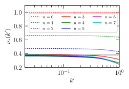
   Figure 9: Plot of $\nu_{*}(k^{\prime})$ vs $k^{\prime}$. The function approaches $\nu_{*}(k^{\prime})\approx 0.38$ (the black horizontal line) asymptotically.

5. The integral of Eq. (68) is performed over the first shell $(k_{1},k_{0})$. Let us denote $\nu_{(1)}(k)$ as the renormalized viscosity after the first step of wavenumber elimination, i.e.,

   $$\nu_{(1)}(k) = \nu_{(0)}(k)+\delta\nu_{(0)}(k).$$ (69)

   We keep eliminating the shells one after the other by the above procedure. After $n+1$ iterations, we obtain

   $$\nu_{(n+1)}(k) = \nu_{(n)}(k)+\delta\nu_{(n)}(k),$$ (70)

   $$\delta\nu_{(n)}(k)k^{2} = \frac{1}{d-1}\int_{\bf{p+q=k}}^{\Delta}\frac{d\mathbf{p}}{(2\pi)^{d}}\frac{B(k,p,q)C(\mathbf{p})}{\nu_{(n)}(p)p^{2}+\nu_{(n)}(q)q^{2}},$$ (71)

   with the integration performed over the $n$-th shell.

6. We compute Eqs. (70, 71) self-consistently. We attempt Kolmogorov’s energy spectrum for the energy, and obtain the renormalized viscosity iteratively (considering that the iteration procedure converges). For the modal energy spectrum $C(\bf p)$, we substitute

   $$C({\bf p})=\frac{2(2\pi)^{d}}{S_{d}(d-1)}p^{-(d-1)}E(p);~{}~{}E(p)=K_{\mathrm{Ko}}\Pi^{2/3}p^{-5/3},$$ (72)

   where $S_{d}$ is the surface area of a $d$-dimensional sphere of unit radius, and $E(p)$ is the one-dimensional Kolmogorov’s spectrum. Regarding $\nu_{(n)}(k)$, we attempt the following form of solution

   $$\nu_{(n)}(k)=\nu_{(n)}(k_{n}k^{\prime})=(K_{\mathrm{Ko}})^{1/2}\Pi^{1/3}k_{n}^{-4/3}\nu_{*(n)}(k^{\prime})$$ (73)

   with $k=k_{n}k^{\prime}$ and $k^{\prime}<1$. The above equation is consistent with $\nu(k)\sim k^{-4/3}$. We expect $\nu_{*(n)}(k^{\prime})$ to be a universal functions for large $n$. Substitutions of the above forms of $C({\bf p})$ and $\nu_{(n)}(k)$ in Eqs. (70, 71) yields the following equations:

   $$\delta\nu_{*(n)}(k^{\prime})=\frac{1}{(d-1)} \int_{\bf{p^{\prime}+q^{\prime}=k^{\prime}}}d\mathbf{q}^{\prime}\frac{2}{(d-1)S_{d}}\frac{E^{u}(q^{\prime})}{q^{\prime d-1}}$$ (74)

   $$\times\left[\frac{S(k^{\prime},p^{\prime},q^{\prime})}{\nu_{*(n)}(hp^{\prime})p^{\prime 2}+\nu_{*(n)}(hq^{\prime})q^{\prime 2}}\right],$$

   $$\nu_{*(n+1)}(k^{\prime})=h^{4/3}\nu_{*(n)}(hk^{\prime})+h^{-4/3}\delta\nu_{*(n)}(k^{\prime}),$$ (75)

   where the integral in the above equation is performed over a region $1\leq p^{\prime},q^{\prime}\leq 1/h$ with the constraint $\mathbf{p}^{\prime}+\mathbf{q}^{\prime}=\mathbf{k}^{\prime}$. Note that $\mathbf{k}^{\prime}=\mathbf{k}/k_{n}$, $\mathbf{p}^{\prime}=\mathbf{p}/k_{n}$, $\mathbf{q}^{\prime}=\mathbf{q}/k_{n}$. Fournier & Frisch (1978) showed the above volume integral in $d$ dimensions is

   $$\int_{\mathbf{p}^{\prime}+\mathbf{q}^{\prime}=\mathbf{k}^{\prime}}d\mathbf{p^{\prime}}=S_{d-1}\int dp^{\prime}dq^{\prime}\left(\frac{p^{\prime}q^{\prime}}{k^{\prime}}\right)^{d-2}\left(\sin\alpha\right)^{d-3},$$ (76)

   where $\alpha$ is the angle between vectors $\mathbf{p}^{\prime}$ and $\mathbf{q}^{\prime}$.

7. $\nu_{*(n)}(k^{\prime})$ is solved iteratively using Eqs. (74-75) with $h=0.7$ (McComb, 1990, 2014; Zhou, 2010). Zhou et al. (1997) showed that the Kolmogorov constant computed using RG is approximately 1.6 independent of $h$, as long as it lies between 0.55 to 0.75. Therefore we choose $h=0.7$ for our computation. We start with a constant value of $\nu_{*(0)}(k^{\prime})$, and compute the integral using Gaussian quadrature. This process is iterated till $\nu_{*(n+1)}(k^{\prime})\approx\nu_{*(n)}(k^{\prime})$, that is, till the solution converges. The result of our RG analysis, exhibited in Fig. 9, shows a constancy of $\nu_{*}(k^{\prime})$ with $k^{\prime}$. A slight downward bend near $k^{\prime}=1$ is attributed to the neglect of the triple nonlinearity of the unresolved modes (see item 1, and Zhou et al. (1988)).

For large $n$, $\nu_{*(n)}(k^{\prime})$ converges asymptotically to $\nu_{*}\approx 0.38$ as $k^{\prime}\rightarrow 0$. The above result is same as that for ${\mathbf{U}}_{0}=0$, thus we conclude that the renormalized viscosity $\nu_{n}(k)$ is independent of $\mathbf{U}_{0}$.

The aforementioned description does not fully match with the numerical simulation described in §2 and §4. In the numerical simulations we showed that the absolute value of the normalised correlation function or the Green’s function decays in time with time scale $1/\nu(k)k^{2}$. However the imaginary part and phase of the correlation function exhibit fluctuations that are related to the sweeping by eddies of larger scales, as predicted by Kraichnan (1964). This sweeping effect is not captured by the Eulerian field theory described above, which was first argued by Kraichnan (1964). Kraichnan (1965) then formulated Lagrangian-history closure approximation for turbulence and showed consistency (also see Leslie, 1973). Also refer to Moriconi et al. (2014) and O’Kane & Frederiksen (2008) for more work on field-theoretic treatment of turbulence. We do not describe this formalism due to limited scope of the present paper.

References

- Batchelor (1971) Batchelor, G. K. 1971 Theory of Homogeneous Turbulence. Cambridge: Cambridge University Press.
- Cholemari & Arakeri (2006) Cholemari, Murali R. & Arakeri, Jaywant H. 2006 A model relating Eulerian spatial and temporal velocity correlations. J. Fluid Mech. 551, 19–11.
- Davidson (2015) Davidson, Peter A. 2015 Turbulence, 2nd edn. Oxford: Oxford University Press.
- DeDominicis & Martin (1979) DeDominicis, C. & Martin, P. C. 1979 Energy spectra of certain randomly-stirred fluids. Phys. Rev. A 19 (1), 419.
- Fournier & Frisch (1978) Fournier, J. D. & Frisch, Uriel 1978 d-dimensional turbulence. Phys. Rev. A 17 (2), 747–762.
- Frisch (1995) Frisch, Uriel 1995 Turbulence. Cambridge: Cambridge University Press.
- He et al. (2016) He, Guowei, Jin, Guodong & Yang, Yue 2016 Space-Time Correlations and Dynamic Coupling in Turbulent Flows. Annu. Rev. Fluid Mech. 49 (1), 15.
- He (2011) He, X. 2011 Kraichnan’s random sweeping hypothesis in homogeneous turbulent convection. Phys. Rev. E 83, 037302.
- He et al. (2010) He, Xiaozhou, He, Guowei & Tong, Penger 2010 Small-scale turbulent fluctuations beyond Taylor’s frozen-flow hypothesis. Phys. Rev. E 81 (6), 065303(R).
- Kolmogorov (1941a) Kolmogorov, Andrey Nikolaevich 1941a Dissipation of Energy in Locally Isotropic Turbulence. Dokl Acad Nauk SSSR 32 (1), 16–18.
- Kolmogorov (1941b) Kolmogorov, Andrey Nikolaevich 1941b The local structure of turbulence in incompressible viscous fluid for very large Reynolds numbers. Dokl Acad Nauk SSSR 30 (4), 301–305.
- Kraichnan (1959) Kraichnan, Robert H. 1959 The structure of isotropic turbulence at very high Reynolds numbers. J. Fluid Mech. 5, 497–543.
- Kraichnan (1964) Kraichnan, Robert H. 1964 Kolmogorov’s Hypotheses and Eulerian Turbulence Theory. Phys. Fluids 7 (11), 1723.
- Kraichnan (1965) Kraichnan, Robert H. 1965 Lagrangian-History Closure Approximation for Turbulence. Phys. Fluids 8 (4), 575–598.
- Landau & Lifshitz (1987) Landau, L D & Lifshitz, E M 1987 Fluid Mechanics. Butterworth-Heinemann.
- Lesieur (2012) Lesieur, M. 2012 Turbulence in Fluids, 4th edn. Dordrecht: Springer.
- Leslie (1973) Leslie, D C 1973 Developments in the Theory of Turbulence. Clarendon Press.
- McComb (1990) McComb, W. D. 1990 The physics of fluid turbulence. Clarendon Press.
- McComb (2014) McComb, W. D. 2014 Homogeneous, Isotropic Turbulence: Phenomenology, Renormalization and Statistical Closures. Oxford: Oxford University Press.
- McComb & Shanmugasundaram (1983) McComb, W. D. & Shanmugasundaram, V. 1983 Fluid turbulence and the renormalization group: A preliminary calculation of the eddy viscosity. Phys. Rev. A 28 (4), 2588–2590.
- McComb & Shanmugasundaram (1984) McComb, W. D. & Shanmugasundaram, V. 1984 Numerical calculation of decaying isotropic turbulence using the LET theory. J. Fluid Mech. 143, 95–123.
- Moriconi et al. (2014) Moriconi, L, Pereira, R M & Grigorio, L S 2014 Velocity-gradient probability distribution functions in a lagrangian model of turbulence. J. Stat. Phys. p. P10015.
- O’Kane & Frederiksen (2008) O’Kane, Terence J & Frederiksen, J S 2008 Statistical dynamical subgrid-scale parameterizations for geophysical flows. Phys. Scripta T132, 014033.
- Pope (2000) Pope, Stephen B. 2000 Turbulent Flows. Cambridge: Cambridge University Press.