Electron-vibron coupling effects on electron transport via a single-molecule magnet

Abstract

We investigate how the electron-vibron coupling influences electron transport via an anisotropic magnetic molecule, such as a single-molecule magnet (SMM) Fe₄, by using a model Hamiltonian with parameter values obtained from density-functional theory (DFT). Magnetic anisotropy parameters, vibrational energies, and electron-vibron coupling strengths of the Fe₄ are computed using DFT. A giant spin model is applied to the Fe₄ with only two charge states, specifically a neutral state with the total spin $S=5$ and a singly charged state with $S=9/2$, which is consistent with our DFT result and experiments on Fe₄ single-molecule transistors. In sequential electron tunneling, we find that the magnetic anisotropy gives rise to new features in conductance peaks arising from vibrational excitations. In particular, the peak height shows a strong, unusual dependence on the direction as well as magnitude of applied $B$ field. The magnetic anisotropy also introduces vibrational satellite peaks whose position and height are modified with the direction and magnitude of applied $B$ field. Furthermore, when multiple vibrational modes with considerable electron-vibron coupling have energies close to one another, a low-bias current is suppressed, independently of gate voltage and applied $B$ field, although that is not the case for a single mode with the similar electron-vibron coupling. In the former case, the conductance peaks reveal a stronger $B$-field dependence than in the latter case. The new features appear because the magnetic anisotropy barrier is of the same order of magnitude as the energies of vibrational modes with significant electron-vibron coupling. Our findings clearly show the interesting interplay between magnetic anisotropy and electron-vibron coupling in electron transport via the Fe₄. The similar behavior can be observed in transport via other anisotropic magnetic molecules.

I Introduction

Recent experimental advances allow individual molecules to be placed between electrodes, and their electron transport properties to be measured in single-molecule junctions or transistors. One interesting family of molecules among them are anisotropic magnetic molecules referred to as single-molecule magnets (SMMs). A SMM comprises a few transition metal ions surrounded by several tens to hundreds of atoms, and has a large spin and a large magnetic anisotropy barrier FRIE96 ; THOM96 ; CHUD98 . Crystals of SMMs have drawn attention due to unique quantum properties such as quantum tunneling of magnetization FRIE96 ; THOM96 and quantum interference or Berry-phase oscillations induced by the magnetic anisotropy WERN99 ; GARG93 ; BURZ13 . There have been studies of the interplay between the quantum properties and the electron transport of individual SMMs at the single-molecule level HEER06 ; LEUE06 ; ROME06 ; TIMM06 ; JO06 ; SALV09 ; ZYAZ10 ; CHUD11 ; TIMM12 ; GANZ13 ; MISI13 ; WU13 ; ROME14 .

Molecules trapped in single-molecule devices vibrate with discrete frequencies characteristic to the molecules, and the molecular vibrations can couple to electronic charge and/or spin degrees of freedom. When this coupling is significant, electrons may tunnel via the vibrational excitations unique to the molecules, and the coupling can be tailored by external means. Electron tunneling through vibrational excitations have been observed in single-molecule devices based on carbon nanotubes GANZ13 ; LERO04 ; SAPM06 ; LETU09 ; BENY14 and small molecules STIP98 ; PARK00 ; YU04 ; LEON08 including SMMs such as Fe₄ BURZ14 . Interestingly, in some cases, a pronounced suppression of a low-bias current was found, attributed to a strong coupling between electronic charge and vibrations of nanosystems SAPM06 ; LETU09 ; BURZ14 ; KOCH05 ; KOCH06 . It was also shown that the coupling strength could be modified at the nanometer scale in carbon nanotube mechanical resonators BENY14 . For a SMM TbPc₂ grafted onto a carbon nanotube, a coupling between the molecular spin and vibrations of the nanotube was observed in conductance maps of the nanotube GANZ13 .

So far, theories of the electron-phonon or electron-vibron coupling effects have been developed only for isotropic molecules KOCH06 ; MITR04 ; GALP07 ; SECK11 ; HART13 ; CORN07 ; FRED07 ; PAUL05 ; MCCA03 ; SELD08 in single-molecule junctions or transistors. For example, for molecules weakly coupled to electrodes, a model Hamiltonian approach is commonly used to investigate the coupling effects, while for molecules strongly coupled to electrodes, a first-principles based method such as density-functional theory (DFT) combined with non-equilibrium Green’s function method, is applied FRED07 . Recently, the coupling effects have been studied for isotropic molecules weakly coupled to electrodes, by using both DFT and the model Hamiltonian approach SELD08 . For anisotropic magnetic molecules weakly coupled to electrodes, a combination of DFT and a model Hamiltonian would be proper to examine the coupling effects. The interplay between magnetic anisotropy and vibron-assisted tunneling can provide interesting features concerning vibrational conductance peaks.

The SMM Fe₄ has been shown to form stable single-molecule transistors without linker groups ZYAZ10 ; BURZ12 ; BURZ14 . The Fe₄ consists of four Fe³⁺ ions (each ion with spin $S_{i}=5/2$), among which the center Fe³⁺ ion is weakly antiferromagnetically coupled to the outer Fe³⁺ ions via O anions, as shown in Fig. 1(a). The neutral Fe₄ has the total ground-state spin $S=5$ with a magnetic anisotropy barrier of 16.2 K [Fig. 1(b)] ACCO06 ; BURZ12 ; BURZ14 , while its doubly degenerate excited spin multiplets $S=4$ are located at 4.8 meV above the ground-state spin multiplet $S=5$ ACCO06 . The negatively singly charged Fe₄ has the total spin $S=9/2$ well separated from the excited spin multiplet $S=11/2$. The previous DFT calculations suggest that the Fe₄ has only three vibrational modes with the electron-vibron coupling greater than unity BURZ14 .

Here we present three electron-vibron coupling effects on electron transport via the SMM Fe₄ at low temperatures, in a sequential electron tunneling limit [Fig. 1(c)], by using the model Hamiltonian with the DFT-calculated magnetic anisotropy parameters, vibrational energies, and electron-vibron coupling strengths. Firstly, the height of vibrational conductance peaks shows a strong, unusual dependence on the direction and magnitude of applied $B$ field. This $B$-field dependence is attributed to the magnetic anisotropy barrier that is of the same order of magnitude as the energies of the vibrational modes with significant electron-vibron coupling. Without the magnetic anisotropy, the conductance peaks would be insensitive to the $B$-field direction. Secondly, satellite conductance peaks of magnetic origin exhibit a unique $B$-field evolution depending on the direction of $B$ field. At low $B$ fields, the low-bias satellite peak arises from the magnetic levels in the vibrational ground state only, while at high $B$ fields, the levels in the vibrational excited states contribute to the satellite peak as much as that those in the vibrational ground state, because the separation between the levels becomes comparable to the vibrational excitations. Thirdly, when multiple modes with significant electron-vibron coupling ($1<\lambda<2$) have energies close to one another, the low-bias conductance peak and the $B$-field dependence of the conductance peaks reveal qualitatively different features from the case of a single mode with the similar electron-vibron coupling. The similar trend to our findings may be observed for any anisotropic magnetic molecules as long as magnetic anisotropy is comparable to vibrational energies. This work can be viewed as a starting point for an understanding of magnetic anisotropy effects on electron tunneling via vibrational excitations, by using the combined method.

The outline of this work is as follows. We present the DFT method in Sec.II, and show our DFT results on electronic structure and magnetic and vibrational properties of the Fe₄ in Sec.III. We introduce the model Hamiltonian and a formalism for solving the master equation in Sec.IV, and discuss calculated transport properties of the Fe₄ as a function of gate voltage, temperature, and applied $B$ field in Sec.V. Finally, we make a conclusion in Sec.VI.

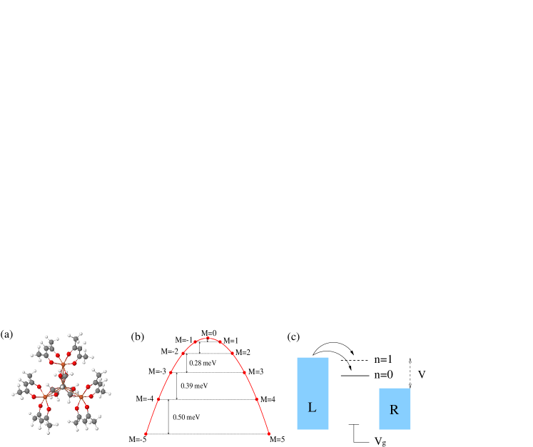
Figure 1: (Color online) (a) Top view of the Fe₄ molecule with $C_{2}$ symmetry axis along the vertical axis, where Fe (orange), O (red), C (gray), H (white). Simplified from Ref.ACCO06 . (b) Magnetic energy levels of the Fe₄ with $S=5$ where the zero-field splitting is 0.50 meV. (c) Schematic view of sequential tunneling from the left electrode to a molecular level ($n=0$: vibrational ground state, $n=1$: vibrational first-excited state), where $V$ is a bias voltage and $V_{g}$ is a gate voltage. The magnetic levels in each vibrational state are not shown. The chemical potential of the left and right electrodes are $+eV/2$ and $-eV/2$, respectively.

II DFT calculation Method

We perform electronic structure calculations of an isolated Fe₄ molecule using the DFT code, NRLMOL NRLMOL , considering all electrons with Gaussian basis sets within the generalized-gradient approximation (GGA) PERD96 for the exchange-correlation functional. To reduce the computational cost, the Fe₄ molecule ACCO06 is simplified by replacing the terminating CH₃ groups by H atoms, and by substituting the phenyl rings (above and below the plane where the Fe ions are located) with H atoms. Figure 1(a) shows the simplified Fe₄ molecule with $C_{2}$ symmetry. Without such simplification, vibrational modes would not be obtained within a reasonable compute time. It is confirmed that this simplification does not affect much the electronic and magnetic properties of the Fe₄ molecule (Sec.III.A). The phenyl rings are known to have high-frequency vibrational modes (about 600-1000 cm^-1) LIU90 , while the electron-vibron coupling is significant for low-frequency vibrational modes. Therefore, the replacement of the phenyl rings by H would not affect our calculation of electron-vibron coupling strengths for low-frequency vibrational modes. The total magnetic moments of the neutral and charged Fe₄ molecules are initially set to 10 $\mu_{B}$ and 9 $\mu_{B}$, respectively, and they remain the same after geometry relaxation. The geometries of the neutral and charged Fe₄ molecules are relaxed with $C_{2}$ symmetry, until the maximum force is less than 0.009 eV/Å, or 0.00018 Ha/$a_{B}$, where $a_{B}$ is Bohr radius. For the relaxed geometry of the neutral Fe₄, we calculate vibrational or normal modes within the harmonic oscillator approximation, using the frozen phonon method NRLMOL . We also calculate the magnetic anisotropy parameters for the neutral Fe₄ molecule by considering spin-orbit coupling perturbatively to the converged Kohn-Sham orbitals and orbital energies obtained from DFT, as implemented in NRLMOL NRLMOL ; PEDE99 .

III DFT results: electronic, magnetic and vibrational properties

III.1 Electronic and magnetic properties

Figure 2: (a) Majority- and (b) minority-spin total and projected density of states onto the center Fe and outer Fe sites and onto all O atoms of the Fe₄ molecule shown in Fig. 1(a). The midpoint between the HOMO and the LUMO levels is set to zero. The arrows in the bottom panel of (b) indicate the HOMO and LUMO levels. Obtained from the neutral Fe₄.

Our DFT calculations show that the neutral Fe₄ molecule with $S=5$ has an energy gap of 0.87 eV between the lowest unoccupied molecular orbital (LUMO) and the highest occupied molecular orbital (HOMO) levels. The HOMO level is doubly degenerate, while the doubly degenerate LUMO+1 level is separated from the LUMO level by 0.05 eV. The LUMO arises from the outer Fe ions with the minority spin (spin down) at the vertices of the triangle [Fig. 1(a)], while the HOMO from the center Fe ion with the minority spin, as shown in Fig. 2. The O orbital levels are found at the same energies as the Fe orbital levels. The contributions of the C and H atoms to the HOMO and LUMO are negligible. The majority-spin HOMO is 0.08 eV below the minority-spin HOMO, and the majority-spin LUMO is 0.23 eV above the minority-spin LUMO. The calculated electronic structure suggests that when an extra electron is added to the Fe₄ molecule, the electron is likely to go to the minority-spin outer Fe sites. Thus, the total spin of the charged Fe₄ is expected to be $S=9/2$, which is consistent with our DFT calculation and experimental data BURZ12 . Furthermore, we calculate the uniaxial ($D$) and transverse magnetic anisotropy ($E$) parameters for the neutral Fe₄, finding that $D$=0.056 meV and $E$=0.002 meV, respectively. These values are in good agreement with the experimental values, $D=0.056$ and $E=0.003$ meV BURZ12 and the previous DFT-calculated result NOSS13 . The calculated magnetic anisotropy barrier for the neutral Fe₄ is 16.2 K ($\sim$1.4 meV) [Fig. 1(b)], in good agreement with experiment ACCO06 ; BURZ12 . The calculated zero-field splitting is 0.5 meV, which is an energy difference between the two lowest doublets in the absence of external $B$ field.

The electronic structure study of the charged Fe₄ molecule, however, provides a HOMO-LUMO gap of 0.06 eV, which agrees with the previous DFT result NOSS13 . This small gap is partially due to the degenerate LUMO levels and partially attributed to delocalization of the extra electron over the Fe₄ (or difficulty in localization of the extra electron). The latter arises from an inherent limitation of DFT caused by the absence of self-interaction corrections PEDE85 . The magnetic anisotropy parameters are highly sensitive to the HOMO-LUMO gap and the location of the extra electron in the Fe₄. Therefore, in our transport calculations (Sec.V), for the charged Fe₄ molecule, we use the DFT-calculated relaxed geometry but not the DFT-calculated magnetic anisotropy parameter values.

III.2 Vibrational spectra and electron-vibron coupling

Figure 3: Calculated (a) Raman and (b) infrared vibrational spectra of the neutral Fe₄ molecule with projections onto all Fe, all O, all C and H atoms replacing the phenyl rings, and the peripheral C and H atoms. The scales of the horizontal axes in (a) differ from those in (b).

We obtain total and projected Raman and infrared spectra by applying the scheme in Ref. PORE96 to the DFT-calculated vibrational modes of the neutral Fe₄ (Fig. 3). There are 16 non-zero frequency normal modes below 50 cm^-1 (or 6.2 meV), among which the lowest-energy mode has a frequency of 14.7 cm^-1. These low-frequency modes are all Raman active [Fig. 3(a)], and they involve with vibrations of Fe atoms and O and C atoms in the peripheral area. We compare our calculated Raman spectra with experimental data in Ref. BOGA09 . The experimental Raman spectrum is for a crystal of Fe₄ molecules with slightly different ligands and only for high-frequency modes ($>200$ cm^-1). The experimental Raman peaks appear at 257, 378, 401, 413, 511, 539, 590 cm^-1, and they are all involved with Fe-O-Fe vibrations or stretch. The corresponding DFT Raman peaks are found at 255, 345, 393, 414, 482, 542 cm^-1, except for 590 cm^-1. Note that these peaks have much lower intensities than the 16 lower-frequency modes, so that some of them are not visible in the scales of Fig. 3(a). Infrared-active modes [Fig. 3(b)] have much higher frequencies than the Raman active modes.

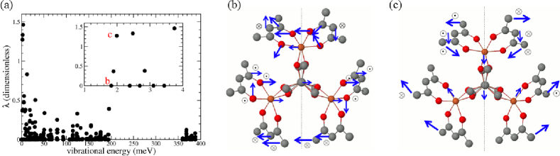
Figure 4: (Color online) (a) Calculated electron-vibron coupling strength vs vibrational energy with an inset of several low-frequency vibrational modes. (b) Vibrational mode “b” and (c) vibrational mode “c” marked in (a), where the arrows represent in-plane displacements and $\bigodot$ and $\bigotimes$ are the positive and negative out-of-plane displacements, respectively. In (b) and (c), the vertical dashed lines are the C₂ symmetry axes. (a) and (c) are adapted from Ref. BURZ14 .

For each vibrational mode, the dimensionless electron-vibron coupling strength is given by MCCA03 ; SELD08 ; BURZ14

$$\lambda = \sqrt{\frac{\omega}{2\hbar}}\mathbf{\Omega}^{T}\mathbf{M}(\mathbf{R}_{0}-\mathbf{R}_{1}),$$ (1)

where $\omega$ is the angular frequency of the mode, $\mathbf{M}$ is a diagonal square matrix of atomic masses, and $\mathbf{\Omega}^{T}$ is a transpose of the mass-weighted normal-mode column eigenvector with $\mathbf{\Omega}^{T}\mathbf{M}\mathbf{\Omega}=1$. Here $\mathbf{R}_{0}$ and $\mathbf{R}_{1}$ are column vectors representing the coordinates of the neutral and charged Fe₄ relaxed geometries, respectively. The relaxed geometries are translated and rotated such that $|\mathbf{R}_{0}-\mathbf{R}_{1}|$ is minimized. Figure 4(a) shows the calculated value of $\lambda$ as a function of vibrational energy $\hbar\omega$. It is found that there are only three normal modes with $\lambda>1$, specifically modes of $\hbar\omega=2.0$, 2.5, 3.7 meV with $\lambda=1.27$, 1.33, 1.46, respectively BURZ14 . The mode “b” in Fig. 4(b) is antisymmetric about the C₂ symmetry axis, while the mode “c” in Fig. 4(c) is symmetric about the C₂ symmetry axis.

IV Model Hamiltonian and master equation

In this section, we present the formalism to calculate transport properties from the model Hamiltonian, adapted from Refs. MITR04 ; KOCH06 to include the molecular spin Hamiltonian and the multiple vibrational modes.

IV.1 Model Hamiltonian

We consider the following model Hamiltonian ${\cal H}={\cal H}_{\rm el}+{\cal H}_{\rm mol}+{\cal H}_{\rm t}$:

$${\cal H}_{\rm el} = \sum_{\alpha=L,R}\sum_{k,\sigma}\epsilon_{k,\sigma}^{\alpha}a_{k,\sigma}^{\alpha{\dagger}}a_{k,\sigma}^{\alpha},\>\>\>\>\>\>{\cal H}_{\rm t}=\sum_{\alpha=L,R}\sum_{k,\sigma}(t_{\alpha}^{\star}c_{\sigma}^{{\dagger}}a_{k,\sigma}^{\alpha}+t_{\alpha}a_{k,\sigma}^{\alpha{\dagger}}c_{\sigma}),$$ (2)

$${\cal H}_{\rm mol} = -D_{N}(S_{z}^{(N)})^{2}+(\epsilon-eV_{g})\sum_{\sigma}c_{\sigma}^{{\dagger}}c_{\sigma}+g\mu_{B}\vec{S}^{(N)}\cdot\vec{B}$$ (3)

$$+\sum_{i}\hbar\omega_{i}d^{{\dagger}}_{i}d_{i}+\sum_{i}\lambda_{i}\hbar\omega_{i}(d^{{\dagger}}_{i}+d_{i})\sum_{\sigma}c_{\sigma}^{{\dagger}}c_{\sigma},$$

where $a_{k,\sigma}^{\alpha{\dagger}}$ and $a_{k,\sigma}^{\alpha}$ are creation and annihilation operators for an electron at the electrode $\alpha$ with energy $\epsilon_{k,\sigma}^{\alpha}$, momentum $\vec{k}$, and spin $\sigma$. Here $c_{\sigma}^{{\dagger}}$ and $c_{\sigma}$ are creation and annihilation operators for an electron with spin $\sigma$ at the molecular orbital $\epsilon$ or the LUMO. The parameter $t_{\alpha}^{\star}$ in ${\cal H}_{\rm t}$ describes electron tunneling from the electrode $\alpha$ to the SMM. Symmetric tunneling is assumed such that $t_{L}=t_{R}$. In ${\cal H}_{\rm mol}$, $D_{N}(>0)$ is the uniaxial magnetic anisotropy parameter for the charge state $N$ with the total spin $S^{(N)}$. The transverse magnetic anisotropy is neglected, since the uniaxial magnetic anisotropy and an applied magnetic field are much greater than the transverse anisotropy. A charging energy of the Fe₄ is about 2.3 eV based on our DFT calculation, and experimental conductance maps show only two Coulomb diamonds ZYAZ10 ; BURZ12 ; BURZ14 . Therefore, we consider only two charge states: the neutral ($N=0$) state with $S=5$ and the singly charged ($N=1$) state with $S=9/2$. The second and third terms in ${\cal H}_{\rm mol}$ represent changing the orbital energy by gate voltage $V_{g}$ and the Zeeman energy with $g=2$, respectively. The second line in ${\cal H}_{\rm mol}$ comprises (a) the energies of independent harmonic oscillators with vibrational angular frequencies $\omega_{i}$ and (b) the coupling between electric charge and vibrational modes with coupling strengths $\lambda_{i}$. Here $d_{i}^{{\dagger}}$ and $d_{i}$ are creation and annihilation operators for the $i$-th quantized vibrational mode or vibron. It is assumed that the vibrational frequencies are not sensitive to the charge state of the Fe₄.

For a weak coupling between the electrodes and the SMM, ${\cal H}_{\rm t}$ is a small perturbation to ${\cal H}_{\rm el}$ and ${\cal H}_{\rm mol}$. Thus, a total wave function $|\Psi\rangle$ can be written as a direct product of a wave function of the electrode $\alpha$, $|\Phi_{\alpha}\rangle$, and the molecular eigenstate $|q\rangle$. Based on the Born-Oppenheimer approximation, the latter can be given by $|\psi^{N}_{m,q}\rangle\otimes|n_{q}\rangle$, where $|\psi^{N}_{m,q}\rangle$ describes an electronic charge and magnetic state and $|n_{q}\rangle$ is a vibrational eigenstate of the SMM with $n_{q}$ vibrons. For $p$ vibrational modes, $n_{q}=n_{1}+n_{2}+...+n_{p}$, where $n_{i}$ is a quantum number of the $i$-th vibrational mode.

When the SMM is charged, the electron-vibron coupling gives rise to off-diagonal terms in the vibrational part of the ${\cal H}_{\rm mol}$ matrix. These terms can be eliminated by applying a canonical transformation MITR04 ; KOCH06 to the Hamiltonian, such as $e^{\hat{Y}}\hat{O}e^{-{\hat{Y}}}$, where $\hat{O}$ is an observable operator and ${\hat{Y}}\equiv-\sum_{i}\lambda_{i}(d^{{\dagger}}_{i}-d_{i})\sum_{\sigma}c_{\sigma}^{{\dagger}}c_{\sigma}$. After the transformation, the molecular Hamiltonian becomes diagonal with respect to the new vibron creation and annihilation operators $d_{i}^{\prime,{\dagger}}$ and $d_{i}^{\prime}$, where $d_{i}^{\prime}=d_{i}+\lambda_{i}\sum_{\sigma}c^{{\dagger}}_{\sigma}c_{\sigma}$. The canonical transformation shifts $\epsilon$ to $\epsilon^{\prime}=\epsilon-\sum_{i}\lambda_{i}^{2}\hbar\omega_{i}$, while $t_{\alpha}$ is modified to $t_{\alpha}\mathrm{exp}[-\sum_{i}\lambda_{i}(d^{{\dagger}}_{i}-d_{i})]$. This energy shift corresponds to a shift of polaron energy caused by adjustment of the ions following the electron tunneled to the molecule. Henceforth, we drop all primes in the operators, parameters, and Hamiltonians.

IV.2 Transition rates

In the sequential tunneling limit [Fig. 1(c)], we write transition rates $R_{i\rightarrow f}$ from the initial state $|\Psi_{i}\rangle$ to the final state $|\Psi_{f}\rangle$, to the lowest order in ${\cal H}_{\rm t}$, as

$$R_{i\rightarrow f} = \frac{2\pi}{\hbar}|\langle\Psi_{f}|{\cal H}_{\rm t}|\Psi_{i}\rangle|^{2}\delta(E_{f}-E_{i}),$$ (4)

$${\cal H}_{\rm t} = \sum_{\alpha=L,R}\sum_{k,\sigma}(t_{\alpha}^{\star}\hat{X}^{{\dagger}}c_{\sigma}^{{\dagger}}a_{k,\sigma}^{\alpha}+t_{\alpha}\hat{X}a_{k,\sigma}^{\alpha{\dagger}}c_{\sigma}),\>\>\>\>\>\hat{X}\equiv\mathrm{exp}[-\sum_{i}\lambda_{i}(d^{{\dagger}}_{i}-d_{i})]$$ (5)

where $E_{f}$ and $E_{i}$ are the final and initial energies, and ${\cal H}_{\rm t}$ is the new tunneling Hamiltonian after the canonical transformation. In these rates we integrate over degrees of freedom of the electrodes and take into account thermal distributions of the electrons in the electrodes by the Fermi-Dirac distribution function $f(E)$. Then the transition rates can be written in terms of degrees of freedom of the SMM only KOCH06 .

Let us first discuss transition rates $\gamma_{\alpha}^{q\rightarrow r}$ from a magnetic level in the $N=0$ state $|q\rangle=|\psi^{N=0}_{M,q},n_{q}\rangle$ to a level in the $N=1$ state $|r\rangle=|\psi^{N=1}_{m,r},n_{r}\rangle$, i.e., electron tunneling from the electrode $\alpha$ to the SMM. The rates are given by

$$\gamma_{\alpha}^{q\rightarrow r} = \sum_{\sigma}W^{\sigma,\alpha}_{q\rightarrow r}f(\bar{\epsilon}-\mu_{\alpha}){\cal F}_{n_{q},n_{r}},$$ (6)

where $W^{\sigma,\alpha}_{q\rightarrow r}$ and ${\cal F}_{n_{q},n_{r}}$ represent transition rates associated with the electronic and nuclear degrees of freedom, respectively. Here $\bar{\epsilon}$ is defined to be $\epsilon_{m}^{N=1}-\epsilon_{M}^{N=0}+(n_{r}-n_{q})\hbar\omega$ for a single vibrational mode, where $\epsilon_{m,M}^{N}$ contain orbital and magnetic energies of the SMM for the charge state $N$. For multiple vibrational modes, indices for individual modes are introduced in $n_{q}$ and $n_{r}$, following the scheme in Refs. SELD11 ; RUHO94 ; RUHO00 . The chemical potential of the left and right electrodes are $\mu_{L}=-\mu_{R}=eV/2$, where $V$ is a bias voltage. In Eq. (6), $f(\bar{\epsilon}-\mu_{\alpha})$ is included in the transition rates since electrons tunnel from the electrode $\alpha$. We discuss the electronic and nuclear parts of the rates separately.

The electronic part of the rates is given by

$$W^{\sigma,\alpha}_{q\rightarrow r} = \frac{2\pi}{\hbar}{\cal D}^{\alpha}_{\sigma}|t_{\alpha}|^{2}|\langle\psi^{N=1}_{m,r}|c^{{\dagger}}_{\sigma}|\psi^{N=0}_{M,q}\rangle|^{2},$$ (7)

$$|\psi^{N=0}_{M,q}\rangle = \sum_{l}u_{l}|S=5,M_{l}\rangle,\>\>\>\>M_{l}=-5,-4,...,4,5,$$ (8)

$$|\psi^{N=1}_{m,r}\rangle = \sum_{j}v_{j}|S=9/2,m_{j}\rangle,\>\>\>\>m_{j}=-9/2,-7/2,...,7/2,9/2,$$ (9)

where ${\cal D}^{\alpha}_{\sigma}$ is the density of states of the electrode ${\alpha}$ near the Fermi level $E_{F}$, which is assumed to be constant and is independent of $\alpha$ and $\sigma$. The initial and final electronic states of the SMM, $|\psi^{N=0}_{M,q}\rangle$ and $|\psi^{N=1}_{m,r}\rangle$, can be expressed as a linear combination of the eigenstates of $S_{z}$ for $S=5$ and $S=9/2$, respectively. The matrix elements $\langle\psi^{N=1}_{m,r}|c^{{\dagger}}_{\sigma}|\psi^{N=0}_{M,q}\rangle$ in $W^{\sigma,\alpha}_{q\rightarrow r}$ dictate selection rules such as $|M-m|=1/2$ and $\Delta N=\pm 1$, and they are evaluated by using the Clebsch-Gordon coefficients.

The nuclear part of the rates, ${\cal F}_{n_{q},n_{r}}$, is called the Franck-Condon factor KOCH06 , and it is symmetric with respect to the indices. The factor is defined to be $|{\cal J}_{n_{q},n_{r}}|^{2}$, where ${\cal J}_{n_{q},n_{r}}$ is an overlap matrix between the nuclear wave functions of the $N=0$ and $N=1$ states KOCH06 ; SELD08 ; SELD11 , i.e.,

$${\cal J}_{n_{q},n_{r}} = \langle n_{r}|\hat{X}|n_{q}\rangle.$$ (10)

In the case of $p$ vibrational modes, for $n_{q}=n_{r}=0$, it is known that

$${\cal J}_{0,0} = \exp[-\sum_{k=1}^{p}\lambda_{k}^{2}/2],\>\>\>\>{\cal F}_{0,0}=\exp[-\sum_{k=1}^{p}\lambda_{k}^{2}].$$ (11)

For the rest of $n_{q}$ and $n_{r}$ values, the overlap matrix elements can be found by applying the following recursion relations RUHO94 ; RUHO00 :

$${\cal J}_{n,n^{\prime}} = -\frac{\lambda_{i}}{\sqrt{n_{i}}}{\cal J}_{n_{i}-1}+\frac{\sqrt{n_{i}^{\prime}}}{\sqrt{n_{i}}}{\cal J}_{n_{i}-1,n_{i}^{\prime}-1}\>\>\>\>\>(n_{i}>0),$$ (12)

$${\cal J}_{n,n^{\prime}} = \frac{\lambda_{i}}{\sqrt{n_{i}^{\prime}}}{\cal J}_{n_{i}^{\prime}-1}+\frac{\sqrt{n_{i}}}{\sqrt{n_{i}^{\prime}}}{\cal J}_{n_{i}-1,n_{i}^{\prime}-1}\>\>\>\>\>(n_{i}^{\prime}>0),$$ (13)

where $n=(n_{1},...,n_{p})$ and $n^{\prime}=(n_{1}^{\prime},...,n_{p}^{\prime})$. In ${\cal J}_{n_{i}-1}$, the quantum number $n_{i}$ is lowered by one with the rest of the quantum numbers fixed, while in ${\cal J}_{n_{i}-1,n_{i}^{\prime}-1}$, both quantum numbers $n_{i}$ and $n_{i}^{\prime}$ are lowered by one with the rest fixed. For example, for a single vibrational mode, we find that ${\cal J}_{0,1}=\lambda e^{-\lambda^{2}/2}$ and ${\cal F}_{0,1}=\lambda^{2}e^{-\lambda^{2}}$.

Now we discuss the transition rates $\gamma_{\alpha}^{r\rightarrow q}$ from the $N=1$ state $|r\rangle=|\psi^{N=1}_{m,r},n_{r}\rangle$ to the $N=0$ state $|q\rangle=|\psi^{N=0}_{M,q},n_{q}\rangle$, i.e., electron tunneling from the SMM to the electrode $\alpha$. Similarly to Eq. (6), the rates are given by

$$\gamma_{\alpha}^{r\rightarrow q} = \sum_{\sigma}W^{\sigma,\alpha}_{r\rightarrow q}[1-f(\bar{\epsilon}-\mu_{\alpha})]{\cal F}_{n_{r},n_{q}},$$ (14)

where $1-f(\bar{\epsilon}-\mu_{\alpha})$ appears since an energy level $\bar{\epsilon}-\mu_{\alpha}$ must be unoccupied for an electron to tunnel back to the electrode $\alpha$.

IV.3 Master equation

A probability $P_{q}$ of the molecular state $|q\rangle$ being occupied, satisfies the master equation

$$\frac{dP_{q}}{dt} = -P_{q}\sum_{\alpha=L,R}\sum_{r}\gamma_{\alpha}^{q\rightarrow r}+\sum_{\alpha=L,R}\sum_{r}\gamma_{\alpha}^{r\rightarrow q}P_{r},$$ (15)

where the summation over $r$ runs for the orbital, magnetic, and vibrational degrees of freedom. The first (second) term sums up all allowed transitions from (to) the state $|q\rangle$. We assume that the vibrons are not equilibrated, in other words, they have a long relaxation time. For steady-state probabilities $P_{q}$, we solve $dP_{q}/dt=0$ by applying the bi-conjugate gradient stabilized method SELD11 ; VORS92 . Starting with the Boltzmann distribution at $V=0$ as initial probabilities, we achieve a fast convergence to the steady-state solution for non-zero bias voltages. Finally, we compute the current $I_{\alpha}$ from the electrode $\alpha$ to the SMM using the steady-state probabilities and transition rates,

$$I_{\alpha=L,R} = e\sum_{q,r}\gamma_{\alpha}^{|N=0,q\rangle\rightarrow|N=1,r\rangle}P_{q}-e\sum_{q,r}\gamma_{\alpha}^{|N=1,r\rangle\rightarrow|N=0,q\rangle}P_{r},$$ (16)

where the sums over $q$ and $r$ run for all the orbital, magnetic, and vibrational indices. In our set-up, the current is positive when an electron tunnels from the left electrode to the SMM (or from the SMM to the right electrode), while it is negative when an electron tunnels from the SMM to the left electrode (or from the right electrode to the SMM). The total current $I=(I_{L}-I_{R})/2$. For symmetric coupling to the electrodes, we have that $I_{L}=-I_{R}$. A differential conductance $dI/dV$ is computed numerically from current-voltage ($I-V$) characteristics by using a small bias interval of $\Delta V=0.01$ or 0.05 mV.

V Results and Discussion: Transport Properties

We present the $I-V$ characteristics and $dI/dV$ vs $V$ as a function of $V_{g}$, temperature $T$, and applied $B$ field, obtained by solving the master equation Eq. (15) with the DFT-calculated parameter values. We use $D_{N=0}=0.056$ meV and $D_{N=1}=0.062$ meV. The value of $D_{N=1}$ is chosen to be 10% greater than the value of $D_{N=0}$, which is consistent with the experimental data BURZ12 . We consider up to 9 vibrons ($n=9$), which is large enough that the transport properties do not change with a further increase of $n$ in the ranges of $V$ and $V_{g}$ of interest. The level broadening $\Gamma=2\pi{\cal D}|t|^{2}$ is taken as 0.01 meV, which satisfies that $\Gamma\ll k_{B}T$, $\hbar\omega$. In the sequential tunneling limit, the $\Gamma$ value plays a role of units in the current and conductance.

Regarding the electron-vibron coupling, we consider two cases: (i) a single vibrational mode with $\lambda>1$, such as $\hbar\omega=2.0$ meV with $\lambda=1.27$ [Fig. 4(c)], and (ii) three vibrational modes with $\lambda>1$, such as $\hbar\omega_{1,2,3}=2.0$, 2.5, 3.7 meV with $\lambda_{1,2,3}=1.27$, 1.33, 1.46 [inset of Fig. 4(a)], which are only modes with $\lambda>1$ from the DFT calculation (Sec.III.B). The case (i) is an instructive example of the electron-vibron coupling. The case (ii) approximates to the case that all of the vibrational modes are included in ${\cal H}_{\rm mol}$, Eq. (3), since the modes with $\lambda<1$ would not significantly contribute to the sequential tunneling at low bias. This is justified because of their exponential contributions to the Franck-Condon factor, Eq. (11). We also confirm that this is the case from actual calculations of the $I-V$ and $dI/dV$ with an additional low-$\lambda$ normal mode to the case (ii). We first present the basic features and magnetic-field dependencies of the conductance peaks for the case (i) and then those for the case (ii).

V.1 Case (i): Basic features

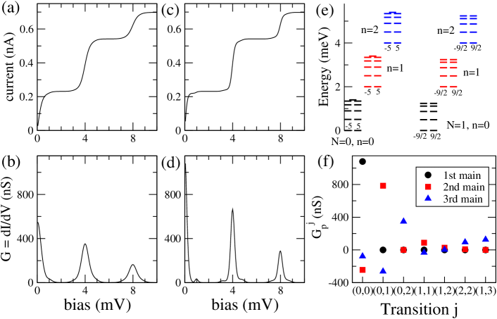
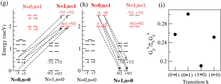
Figure 5: (Color Online) Calculated $I-V$ and $dI/dV$ vs $V$ at the charge degeneracy point for the case (i) at $T=1.16$ K [(a),(b)] and $T=0.58$ K [(c),(d)]. (e) Magnetic energy levels in the vibrational $n=0$, $n=1$, and $n=2$ states for the two charge states $N=0$ and $N=1$. For each set of the magnetic levels, the left column, the center, and the right column correspond to the levels $M<0$, $M=0$, and $M>0$, respectively. (f) Contributions of different transitions $j$ to the first (leftmost), second, and third main $dI/dV$ peak heights in (d). See the main text for the definitions of the transitions ($n$,$n^{\prime}$). (g) and (h) Dominant transition pathways for the transitions (0$\rightarrow$1) and (1$\rightarrow$0). (i) Contributions of transitions $k$ within the transitions ($n=0$,$n^{\prime}=1$) to the height of the second main peak in (d).

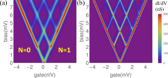
Figure 6: (Color Online) Calculated $dI/dV$ maps as a function of $V$ and $V_{g}$ for the case (i) at $T=1.16$ K (a) and $T=0.58$ K (b).

Figures 5(a)-(d) show the $I-V$ curve and $dI/dV$ vs $V$ for the case (i) at $T=1.16$ K and 0.58 K ($\sim 0.05$ meV), for the gate voltage where the lowest magnetic levels of the $N=0$ and $N=1$ charge states are degenerate at zero bias, i.e., charge degeneracy point. This gate voltage is set to zero. The steps in the current and the $dI/dV$ peaks appear at $V=2n\hbar\omega$ ($n=0$,1,2,…), where the factor of 2 is due to the symmetric bias application [Fig. 1(c)]. The first peak at $V=0$ arises from the vibrational ground state ($n=0$), while the second and third peaks at $V=4.0$ and 8.0 mV come from vibrational excitations ($n=1$ and $n=2$), respectively. Figures 6(a) and (b) reveal $dI/dV$ ($=G$) maps as a function of $V$ and $V_{g}$, i.e., stability diagrams, at 1.16 K and 0.58 K, respectively. Here the Coulomb diamond edges arise from the sequential tunneling via the lowest doublets in the $n=0$ state, while the evenly spaced peaks parallel to the Coulomb diamond edges originate from the vibrational excitations. As $T$ is lowered, overall features of the peaks do not change, while the peaks become sharper with more apparent fine structures.

We now analyze the heights of the $dI/dV$ peaks at 0.58 K in detail [Fig. 5(d)]. The $dI/dV$ peak height decreases as $n$ increases. This implies that the sequential tunneling via the vibrational ground states is dominant over the tunneling via the vibrational excitations for $\lambda=1.27$. This feature qualitatively differs from the case (ii) (Sec.V.C). A peak height at a fixed temperature is determined by the Franck-Condon factor, the electronic part of the transition rates, and the occupation probabilities. We introduce simplified notations for transitions between the $N=0$ and $N=1$ states: ($n$,$n^{\prime}$)$\equiv$ $\{|\psi^{N=0}_{M}\rangle\otimes|n\rangle\rightarrow|\psi^{N=1}_{m}\rangle\otimes|n^{\prime}\rangle$, $|\psi^{N=0}_{M}\rangle\otimes|n\rangle\leftarrow|\psi^{N=1}_{m}\rangle\otimes|n^{\prime}\rangle$, $|\psi^{N=0}_{M}\rangle\otimes|n^{\prime}\rangle\rightarrow|\psi^{N=1}_{m}\rangle\otimes|n\rangle$, $|\psi^{N=0}_{M}\rangle\otimes|n^{\prime}\rangle\leftarrow|\psi^{N=1}_{m}\rangle\otimes|n\rangle\}$ $\equiv$ $\{(n\rightarrow n^{\prime}),(n\leftarrow n^{\prime}),(n^{\prime}\rightarrow n),(n^{\prime}\leftarrow n)\}$. Here ($n$,$n^{\prime}$) contain all possible tunneling paths including all magnetic levels allowed by the selection rules. Several values of the Franck-Condon factor for ($n$,$n^{\prime}$), are listed in Table 3 in the Appendix.

Figure 5(f) shows contributions of different transitions ($n$,$n^{\prime}$) to the first, second, and third peak heights, $G_{p}^{(n,n^{\prime})}$. For the first peak height, only transitions ($n=0,n^{\prime}=0$) contribute. Resonant tunneling occurs via the lowest doublets ($M=\pm 5$ and $m=\pm 9/2$) in the $n=0$ state because they are only occupied levels at 0.58 K. The zero-field splitting is one order of magnitude larger than the thermal energy, and so levels other than the doublets are not occupied [Figs. 1(b),5(e)].

Regarding the second peak height, transitions ($n=0$,$n^{\prime}=1$) dominantly contribute, while transitions ($n=1$,$n^{\prime}=1$) slightly involve in the tunneling [Fig. 5(f)]. In this case, all the levels in the $n=0$ state and some low-lying levels in the $n=1$ are occupied. At $V=4.0$ mV, the transitions ($n=0$,$n^{\prime}=0$) lower the second peak height because the occupation probabilities of the levels in the $n=0$ state differ from those in the case of zero bias. When all the contributions are summed, the second peak is found to have a smaller height than the first peak. Let us discuss in detail the tunneling via ($n=0$,$n^{\prime}=1$) at $V=4.0$ mV. The contributions of ($n=0$,$n^{\prime}=1$) can be decomposed into those of ($0\rightarrow 1$), ($0\leftarrow 1$), ($1\rightarrow 0$), and ($1\leftarrow 0$), as shown in Fig. 5(i). The transition ($0\leftarrow 1$) gives the highest peak value $G_{p}$ among the four transitions. In the case of ($0\rightarrow 1$), as shown in Fig. 5(g), each of the levels $M=\pm 4,\pm 3,\pm 2,\pm 1,0$ in the $n=0$ state can tunnel to two $m$ levels in the $n=1$ state, such as $M=-4$ in the $n=0$ state to $m=-7/2,-9/2$ in the $n=1$ state, but the lowest level $M=5$ ($M=-5$) in the $n=0$ state can transit only to one $m$ level in the $n=1$ state such as $m=9/2$ ($m=-9/2$). However, for the reverse transition, ($0\leftarrow 1$), each of all levels in the $n=1$ state can tunnel to two $M$ levels in the $n=0$ state. In addition, the separation between the level $m=-9/2$ in the $n=1$ state and the level $M=-4$ in the $n=0$ state is $\hbar\omega-9D_{0}$ which is less than $\hbar\omega$. These two factors are the reasons that the contribution of ($0\leftarrow 1$) to the $G_{p}$ is higher than that of ($0\rightarrow 1$). An interesting case is the transition ($1\rightarrow 0$) shown in Fig. 5(h). In this case, two of the allowed transitions require a higher bias voltage than 4.0 mV. The energy difference between the level $M=-4$ ($M=4$) in the $n=1$ state and the level $m=-9/2$ ($m=9/2$) in the $n=0$ state is $\hbar\omega+9D_{0}$. This energy difference prevents the levels $M=\pm 4$ in the $n=1$ state from being significantly occupied at $eV/2=\hbar\omega$. As a consequence, the transition ($1\rightarrow 0$) participates in the tunneling much less than the other three transitions, as confirmed in Fig. 5(i).

For the third peak height, transitions ($n=0$,$n^{\prime}=2$) play a leading role, with considerable contributions of transitions ($n=1$,$n^{\prime}=3$) and ($n=2$,$n^{\prime}=2$) [Fig. 5(f)]. At $V=8.0$ mV, all the levels in the $n=0$ and $n=1$ states as well as some low-lying levels in the $n=2$ and $n=3$ states are involved in the tunneling. The occupation of the levels in the $n=2$ and $n=3$ states significantly modifies the occupation of the levels in $n=0$ and $n=1$ states compared to the case of $V=4.0$ mV. Accordingly, this modification causes the transitions ($n=0$,$n^{\prime}=0$) and ($n=0$,$n^{\prime}=1$) to contribute to the third peak height less than in the case of $V=4.0$ mV. Overall, when all the contributions are added, the third peak has a smaller height than the second peak.

We now examine the magnetic anisotropy effect on the $dI/dV$ map at 0.58 K, as shown in Figs. 5(d) and 6(b). The small (or satellite) peak at 1.0 mV and the flat shoulders around the second and third main peaks in Fig. 5(d), are signatures of the magnetic anisotropy. Since the zero-field splitting (0.5 meV) is a maximum energy difference between adjacent levels for a given $N$ and $n$ state, at a bias voltage of 1.0 mV, all $M$ and $m$ levels in the $n=0$ state are accessible. Thus, all the levels in the $n=0$ state are equally occupied and they contribute to the satellite peak at 1.0 mV. Additional satellite peaks are not found despite increasing a bias voltage, until some low-lying levels in the $n=1$ state become occupied. The left-hand (right-hand) shoulder of the second main peak in Fig. 5(d) is attributed to tunneling to the lowest doublet in the $n=1$ ($n=2$) state barely occupied.

V.2 Case (i): Magnetic field dependence

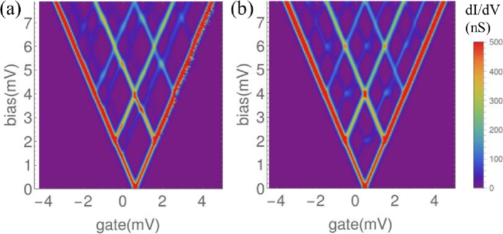
Figure 7: (Color online) Calculated $dI/dV$ values as a function of $V$ and $V_{g}$ for the case (i) at $T=0.58$ K for $B_{z}=8$ T (a) and $B_{x}=8$ T (b). (c) and (d) Computed $dI/dV$ vs $V$ at the charge degeneracy point in (a) and (b), respectively.

Figures 7(a)-(b) are stability diagrams for the case (i) at 0.58 K for $B_{z}=8.0$ T and $B_{x}=8.0$ T, respectively. The zero-bias charge degeneracy for $B_{z}=8.0$ T and $B_{x}=8.0$ T occurs at the gate voltage of 0.61 and 0.46 mV, respectively, due to the Zeeman energy. With an external $B$ field, it is found that the Coulomb diamonds are simply horizontally shifted from the zero $B$-field case, in other words, that the positions of the main $dI/dV$ peaks remain the same relative to the charge degeneracy point. Compare Figs. 7(a)-(b) with Fig. 6(b). Figures 7(c)-(d) exhibit the $dI/dV$ vs $V$ at the charge degeneracy point for $B_{z}=8.0$ T and $B_{x}=8.0$ T, respectively. Compare Figs. 7(c)-(d) with Fig. 5(d). The shift of the main peaks was observed in experiment BURZ14 , and it is consistent with the vibrational origin of the main peaks.

A further comparison between Figs. 7(c)-(d) with Fig. 5(d) reveals two interesting aspects of the $B$-field dependence of the peaks: (1) The heights of the main peaks are greatly modified with the direction as well as magnitude of applied $B$ field, which is a signature of the magnetic anisotropy; (2) Both the positions and the heights of the satellite peaks strongly depend on the direction and magnitude of applied $B$ field. Note that the two effects are found because the magnetic anisotropy barrier or the zero-field splitting is on the same order of magnitude as the vibrational energy. In this section, we present features of the main peak height for the case (i) as a function of $B$ field followed by those of the positions and the heights of the satellite peaks, by considering two $B$-field orientations ($z$ and $x$ axes) for $0\leq B\leq 24.0$ T. Our calculations are carried out at 0.58 K and at a gate voltage corresponding to the charge degeneracy point for each $B$-field value.

V.2.1 $B_{z}$-field dependence of main peaks

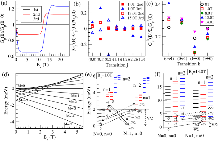
Figure 8: (Color online) (a) Ratio of the heights of the first (black), second (red), and third (blue) main $G=dI/dV$ peaks at $B_{z}$ to the heights of the corresponding $B=0$ peaks, $G_{p}(B)/G_{p}(0)$, vs $B_{z}$ for the case (i) at 0.58 K. (b) Changes of contributions of different transitions $j$ to the second and third main peaks $[G_{p}^{j}(B)-G_{p}^{j}(B=0)]$, relative to the zero $B$ case, normalized by the height of the second and third main peaks at zero $B$, $G_{p}(0)$, computed at $B_{z}=1.0$, 13.0, and 15.0 T. (c) Contributions of transitions $k$ within the transitions ($n=0$,$n^{\prime}=1$) to the second peak at $B_{z}=0,1.0,8.0,13.0$, and 14.0 T. (d) Evolution of the magnetic levels of $S=5$ with $B_{z}$. (e) Dominant transition pathways for the second peak ($V/2=2.0$ mV) at $B_{z}=1.0$ T, where the solid arrow indicates the pathway critical to the abrupt reduction of the second peak height in (a)-(c). (f) Dominant transition pathways for the second peak at $B_{z}=13.0$ T dictating the sudden jump in the second peak height. In (e) and (f), the vertical arrows represent half of the peak bias voltage.

Figure 8(a) shows a ratio of the peak height $G_{p}$ at $B_{z}\neq 0$ to that at zero $B$, $G_{p}(B)/G_{p}(0)$, as a function of $B_{z}$, for the first, second, and third main peaks. The heights of the second and third main peaks decrease abruptly at low $B$ and they remain unchanged until about 12.0 T, above which there appear large steep rises in the heights. The effect of $B_{z}$ is greater on the ratio of the third peak height than on the ratio of the second peak height. However, the first peak height does not change with $B_{z}$ field because only the lowest levels ($M=-5$, $m=-9/2$) in the $n=0$ state participate in the tunneling even for $B_{z}\neq 0$.

Firstly, we study the $B_{z}$-field dependence of the second peak height by understanding how the contributions of transitions $j$ to the height are modified with $B_{z}$ relative to the $B=0$ case, i.e., by computing $[G_{p}^{j}(B)-G_{p}^{j}(B=0)]/G_{p}(0)$, where $j=(n,n^{\prime})$, as shown in Fig. 8(b). It is found that the sharp decrease of the height at low $B$ ($\sim$1.0 T) is mainly caused by a large decrease of the transitions ($n=0,n^{\prime}=1$) at $V=4.0$ mV. For further analysis, we compute $G_{p}^{k}(B)/\sum_{k}G_{p}^{k}(0)$ at several $B_{z}$ values, where $k=$($0\rightarrow 1$), ($0\leftarrow 1$), ($1\rightarrow 0$), ($1\leftarrow 0$). As shown in Fig. 8(c), the large decrease of the transitions ($n=0,n^{\prime}=1$) at low $B_{z}$ is attributed to a large decrease of the transition ($1\rightarrow 0$) compared to the $B=0$ case. This decrease can be understood by examining the evolution of the magnetic levels with $B_{z}$. At zero $B$, within $V=4.0$ mV, several low-lying levels, such as $M=\pm 5$, $\pm 4$ in the $n=0$ ($n=1$) state and $m=\pm 9/2$, $\pm 7/2$ in the $n=1$ ($n=0$) state, dominantly participate in the transitions ($n=0,n^{\prime}=1$). As $B_{z}>0$ increases, the $M,m<0$ levels are shifted down, while the $M,m>0$ levels are lifted up in energy [Fig. 8(d)]. At $B$ field somewhat above $B_{z}=D_{1}/g\mu_{B}=0.54$ T, the $M=5$, 4 and $m=9/2$, 7/2 levels are located quite above the $M=-5$, $-4$ and $m=-9/2$, $-7/2$ levels. Hence, within the bias window, the $M=-5$, $-4$ levels in the $n=0$ ($n=1$) state and the $m=-9/2$, $-7/2$ levels in the $n=1$ ($n=0$) state dominantly contribute to the transitions ($n=0,n^{\prime}=1$), as shown in Fig. 8(e). The separation between the $M=-4$ level in the $n=1$ state and the $m=-9/2$ level in the $n=0$ state, equals $\hbar\omega+(g\mu_{B}B_{z}+9D_{0})$. Since this separation is greater than $V/2$, the occupation of the $M=-4$ level in the $n=1$ state decreases, and the transition ($1\rightarrow 0$) also decreases. As a result, the transition ($n=0,n^{\prime}=1$) considerably decreases, which leads to the drop of the second peak height at low $B$ ($\sim$1.0 T). As $B_{z}$ field increases beyond 1.0 T, the separation between the two lowest levels in a given $N$ and $n$ state grows. Considering the occupation probabilities and the transition rates, within $V=4.0$ mV, the contributions of transitions ($0\rightarrow 1$), ($0\leftarrow 1$), ($1\rightarrow 0$), and ($1\leftarrow 0$) remain almost the same as the case of $B_{z}=1.0$ T [Fig. 8(c)]. Thus, the second peak height does not decrease beyond $B_{z}=1.0$ T. However, the situation dramatically changes when the $B_{z}$ field is high enough that the spacing between the two lowest levels for a given $N$ and $n$ state equals $\hbar\omega$ [Fig. 8(f)]. This occurs at $B=(\hbar\omega-9D_{0})/(g\mu_{B})$ which is 12.9 T. In this case, the $M=-4$ ($m=-7/2$) level in the $n=0$ state is degenerate with the $M=-5$ ($m=-9/2$) level in the $n=1$ state. Thus, at $V=2\hbar\omega$, the occupation of the six levels within the bias window increases compared to the case of lower $B_{z}$ fields, which results in an increase of the transition ($0\rightarrow 1$). Dominant tunneling pathways are indicated in Fig. 8(f). More contributions from the transition ($0\rightarrow 1$) lead to a large increase of the transitions ($n=0,n^{\prime}=1$) at high $B$ fields ($>12.0$ T). Therefore, the peak height sharply rises above 12.0 T.

Secondly, we examine the height of the third peak. Figure 8(b) reveals that within $V=8.0$ mV, at low $B_{z}$, there appear a large decrease of transitions ($n=0$,$n^{\prime}=2$) and a small decrease of transitions ($n=1$,$n^{\prime}=3$) and ($n=2$,$n^{\prime}=2$), despite an increase of ($n=0,n^{\prime}=1$). The overall height is governed by the transitions ($n=0$,$n^{\prime}=2$). Similarly to the second peak height, ($n=0$,$n^{\prime}=2$) can be decomposed into four sets such as ($0\rightarrow 2$), ($0\leftarrow 2$), ($2\rightarrow 0$), and ($2\leftarrow 0$). The trend of the contribution of each of the four sets is similar to the case of the second peak if the $n=1$ state is replaced by the $n=2$ state in the explanation. At low $B_{z}$, the lift of the degeneracy in the low-lying levels above $B_{z}=$0.54 T drives a large reduction of the transition ($2\rightarrow 0$), which results in the rapid drop in the peak height. The peak height does not change beyond $B_{z}=2.0$ T, until the $B_{z}$ field is increased to the field where the spacing between the two lowest levels for a given $N$ and $n$ state is comparable to $\hbar\omega$, similarly to the second peak. At this $B$ field (12.9 T), the second excited level in the $n=0$ state ($M=-3$ or $m=-5/2$) and the first excited level in the $n=1$ state ($M=-4$ or $m=-7/2$) are almost degenerate with the lowest level in the $n=2$ state ($M=-5$ or $m=-9/2$) [Fig. 8(f)]. Hence, at $V=8.0$ mV, the occupation of the levels within the bias window substantially increases, which gives rise to a significant increase of the transition ($0\rightarrow 2$) compared to the zero $B$-field and low $B$ cases, in other words, an increase of the transitions ($n=0$,$n^{\prime}=2$) [Fig. 8(b)]. Consequently, the height of the third peak sharply rises with $B_{z}$ field before its saturation.

V.2.2 $B_{x}$-field dependence of main peaks

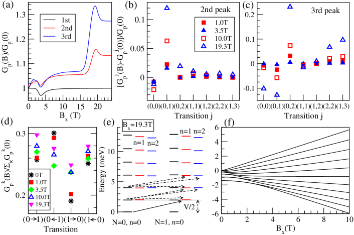
Figure 9: (Color online) (a) Ratio $G_{p}(B)/G_{p}(B=0)$ for the first, second, and third main peaks as a function of $B_{x}$ for the case (i) at 0.58 K. (b) and (c) $[G_{p}^{j}(B)-G_{p}^{j}(B=0)]/G_{p}(0)$ vs transitions $j$ for the second and third peaks at 1.0, 3.5, 10.0, and 19.3 T. (d) Contributions of transitions $k$ within the transitions ($n=0$,$n^{\prime}=1$) to the second peak at $B_{x}=0,1.0,3.5,10.0$, and 19.3 T. (e) Dominant transition pathways for the second peak ($V/2=2.0$ mV) at $B_{z}=19.3$ T, where the solid arrow indicates the pathway contributing most to the abrupt increase of the second peak height in (a) and (b). (f) Evolution of the magnetic levels of $S=5$ with $B_{x}$.

Figure 9(a) shows the ratio $G_{p}(B)/G_{p}(B=0)$ as a function of $B_{x}$, for the first, second, and third main peaks. As $B_{x}$ field increases, the first peak height slightly decreases at low $B$ (2.0-3.5 T) and it returns to the value $G_{p}(0)$. The heights of the second and third main peaks have a complex $B_{x}$ dependence. The heights initially increase somewhat and they slightly decrease at low $B_{x}$ (2.0-3.5 T). Then they gradually increase and jump up from $\sim$17.0 T. After reaching maxima near 19.3 T, the heights slightly go down before saturation. The $B_{x}$-field dependence qualitatively differs from the $B_{z}$-field dependence, which is due to the magnetic anisotropy. Compare Fig. 9(a) with Fig. 8(a).

Firstly, we discuss the first peak height. With a $B_{x}$ field, the magnetic eigenstates are admixtures of different $M_{l}$ levels ($m_{l}$ levels) for $N=0$ state ($N=1$ state), where $M_{l}$ and $m_{l}$ are the eigenstates of $S_{z}$. In contrast to the case of $B_{z}$ field, for small $B_{x}$ fields, several low-lying levels for a given $N$ and $n$ state remain degenerate within the thermal energy, $k_{B}T=$0.05 meV ($\sim$0.58 K) [Fig. 9(f)]. For example, around $B_{x}=1.0$ T (2.0 T), there are three (two) low-lying doublets for a given $N$ and $n$ state [Fig. 9(f)]. However, when the $B_{x}$ field increases above 3.0 T, the degeneracy of all the levels is lifted, and the separation between the adjacent levels grows with $B_{x}$. At $V=0$, for zero $B$, only the lowest doublet in the $N$ and $n=0$ state participate in the tunneling, while for $B_{x}=$2.0-3.0 T, the first-excited level in the $N$ and $n=0$ state slightly contributes to the peak, which causes the small decrease of the peak height. When the first-excited level is well separated from the lowest level in the $n=0$ state at higher $B_{x}$ fields, the peak height resumes to the $G_{p}(0)$ value.

Secondly, let us examine the second peak height by computing $[G_{p}^{j}(B)-G_{p}^{j}(0)]/G_{p}(0)$, where $j=$($n$,$n^{\prime}$), as shown in Fig. 9(b). It is found that the $B_{x}$-field dependence of the peak height is mainly determined by a $B_{x}$-field dependence of the transitions ($n=0$,$n^{\prime}=1$). At low $B_{x}$ ($\sim$1.0 T), for $V=4.0$ mV, the transition (0$\leftarrow$1) is dominant among the four possible transitions within ($n=0$,$n^{\prime}=1$) [Fig. 9(d)]. This feature is similar to the zero $B$-field case since there are still a few degenerate pairs for a given $N$ and $n$ state within $V=4.0$ mV. As $B_{x}$ increases above 3.5 T, the degeneracy of the levels is completely lifted, and so the transition (0$\leftarrow$1) used to dominantly contributing to the peak in zero $B$ field now decreases. However, the strong mixing between different $M_{l}$ or $m_{l}$ levels in the eigenstates open up more tunneling pathways within the bias window than the $B_{z}$ case. As a result, the transition (1$\rightarrow$0) used to be suppressed at zero $B$ field and $B_{z}$ fields now increases [Fig. 9(d)]. With a further increase of $B_{x}$, the three transitions other than (1$\rightarrow$0) increase, and so the peak height goes up. As $B_{x}$ field increases above 17.0 T, the spacing between the first-excited and the lowest levels for a given $N$ and $n$ state becomes close to $\hbar\omega$, which creates more tunneling paths. For example, at 19.3 T, the first-excited level in the $n=0$ state has the same energy as the lowest level in the $n=1$ state, and so the occupation of the levels within the bias window [Fig. 9(e)] is higher than the lower $B_{x}$-field case. At $V=4.0$ mV, the increase of the occupation makes the transitions ($n=0$,$n^{\prime}=1$) contribute more to the peak height and it also allows the transitions ($n=0$,$n^{\prime}=2$) to participate in the tunneling. Thus, the second peak height reaches the maximum. Some dominant tunneling pathways are indicated in Fig. 9(e).

Thirdly, we examine the height of the third peak. The $B_{x}$-field dependence of the peak height dominantly arises from a $B_{x}$-field dependence of the transitions ($n=0$,$n^{\prime}=2$), as shown in Fig. 9(c). Within $V=8.0$ mV, at $B_{x}=$ 3.5 T, the transitions (0$\leftarrow$2) and (2$\leftarrow$0) decrease as much as transitions (0$\rightarrow$2) and (2$\rightarrow$0) increase, among the transitions ($n=0$,$n^{\prime}=2$), so that the peak height is close to the $G_{p}(0)$ value. As $B_{x}$ field increases further, the low-lying levels in the $n=0$ state become close to the low-lying levels in the $n=2$ state. At 19.3 T, the second-excited level in the $n=0$ state and the first-excited level in the $n=1$ state are almost degenerate with the lowest level in the $n=2$ state [Fig. 9(e)]. Thus, for $V=8.0$ mV, the increase in the occupation of the levels within the bias window greatly enhances the tunneling via the transitions ($n=0$,$n^{\prime}=2$) and somewhat increases the transitions ($n=1$,$n^{\prime}=3$) and ($n=2$,$n^{\prime}=2$). The overall peak height becomes the maximum despite a decrease of the transitions ($n=0$,$n^{\prime}=0$) and ($n=0$,$n^{\prime}=1$). Small contributions of new transitions ($n=0$,$n^{\prime}=3$), ($n=1$,$n^{\prime}=4$), ($n=3$,$n^{\prime}=4$) to the third peak at 19.3 T are reduced when $B_{x}$ field further increases.

V.2.3 $B_{z}$-field dependence of satellite peaks

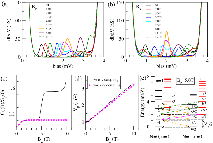
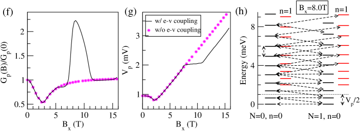
Figure 10: (Color online) (a) $B_{z}$-field and (b) $B_{x}$-field evolution of the satellite conductance peaks between the first and second main peaks. (c) and (d) Height and position of the leftmost satellite peak vs $B_{z}$ with and without the electron-vibron coupling. (e) Dominant tunneling pathways for the leftmost satellite peak at $B_{z}=5.0$ T, where the solid magenta arrow indicates the transition determining the peak bias. (f) and (g) Height and position of the leftmost satellite peak vs $B_{x}$ with and without the electron-vibron coupling. (h) Dominant tunneling pathways for the leftmost satellite peak at $B_{x}=8.0$ T, where the vertical arrows indicate half of the peak bias.

The $B_{z}$-field evolution of the satellite peaks is shown in Fig. 10(a). As $B_{z}$ increases, interestingly, the leftmost satellite peak and the satellite peak on the right side of the second main peak move toward a higher bias voltage, while the satellite peak on the left side of the second main peak is shifted toward a lower bias voltage. Starting from the leftmost one, the satellite peaks are referred to as first, second, and third. Around 4.5 T, the first and the second satellite peaks merge into one peak, and the merged peak moves toward a higher bias voltage. The merged satellite peak disappears above 10.0 T.

Let us focus on the field evolution of the heights and positions of the first and the second satellite peaks. For $B_{z}>0.5$ T, the peak bias $V_{p}$ for the leftmost satellite peak is dictated by the separation between the two lowest levels $M=-4$ and $M=-5$ (or $m=-7/2$ and $m=-9/2$) in the $n=0$ state, which grows linearly with $B_{z}$, i.e., $V_{p}(B)/2=\mathrm{min}\{(9D_{0}+g\mu_{B}|B_{z}|),(8D_{1}+g\mu_{B}|B_{z}|)\}$, as shown in Fig. 10(d). However, the second satellite peak is governed by a bias voltage where a few low-lying levels in the $n=1$ state are just about to be populated. The low-lying levels of the $n=1$ state become closer to the first-excited level in the $n=0$ state, as $B_{z}$ increases. Therefore, with an increase of $B_{z}$, a smaller bias voltage can induce a tiny occupation in the low-lying levels of the $n=1$ state, shifting the position of the second satellite peak to the opposite direction to the first satellite peak. More specifically, for $B_{z}\lesssim 4.0$ T, the tunneling between the levels in the $n=0$ state and the levels $n=1$ states is prevented within the first satellite peak bias. However, at $B_{z}\gtrsim 4.5$ T, several low-lying levels in the $n=0$ and $n=1$ states are sufficiently close to one another, and so the transitions ($n=0$,$n^{\prime}=1$) are allowed within the bias window [Fig. 10(e)]. Thus, for $B_{z}\sim 4.5$ T, the first and second satellite peaks merge, and the transitions ($n=0,n^{\prime}=1$) begin to significantly contribute to the merged satellite peak in addition to the transitions ($n=0,n^{\prime}=0)$. For higher $B_{z}$ fields, the contributions of the transitions ($n=0,n^{\prime}=1$) to the merged peak outweigh those of the transitions ($n=0,n^{\prime}=0)$. This explains the abrupt large increase of the height of the merged peak and the sudden small jump in the intercept of the $V_{p}$ curve starting from 4.5-5.0 T. Thus, the position and the height of the leftmost satellite peak become largely deviated from the case of without electron-vibron coupling, as shown in Figs. 10(c) and (d).

We can estimate the $B_{z}$ value from which the satellite peaks begin to merge. According to the analysis of the transitions ($n=0,n^{\prime}=1$) similar to that in Sec.V.B.1, at low and intermediate $B_{z}$ fields, the transitions (0$\rightarrow$1) and (0$\leftarrow$1) contribute more than the transitions (1$\rightarrow$0) and (1$\leftarrow$0), within the bias window [Fig. 8(c)]. Therefore, the minimum $B_{z}$ value where the satellite peaks merge can be determined by the minimum bias window which allows the transition between the level $M=-4$ in the $n=0$ state and the level $m=-9/2$ in the $n=1$ state, that is, $B_{z}=[\hbar\omega/2-9D_{0}]/g\mu_{B}$ [the solid arrow in Fig. 10(e)]. This value is 4.3 T, which agrees with what we find from the actual calculation of the $dI/dV$ vs $V$. The merged satellite peak, however, disappears when the spacing between the two lowest levels for a given $N$ and $n$ state is comparable to $\hbar\omega$, since in this case the second main peak appears at the same bias voltage. Even though the first-excited level in the $n=0$ state is degenerate with the lowest-level in the $n=1$ state at 12.9 T, the merged satellite peak cannot be identified above 10.0 T due to the broadening of the second main peak.

V.2.4 $B_{x}$-field dependence of satellite peaks

With a $B_{x}$ field, similarly to the case of $B_{z}$ field, the first and second satellite peaks are shifted toward the opposite directions, merging into one, until the merged peak disappears $B_{x}\gtrsim$16.0 T, as shown in Fig. 10(b). However, the leftmost satellite peak has distinctive features from the case of $B_{z}$ field: (1) The peak height forms a large protrusion for 7.5 $\lesssim B_{x}\lesssim$ 11.0 T after which it decreases to the $G_{p}(0)$ value; (2) The peak voltage remains almost flat for 7.0 $\lesssim B_{x}<$ 11.0 T; (3) The peak disappears at a higher $B_{x}$ field than in the case of $B_{z}$ field. Compare Figs. 10(f) and (g) with Figs. 10(c) and (d).

We discuss the leftmost satellite peak first for $B_{x}\lesssim$ 11.0 T and then for higher $B_{x}$ fields. The unique features of the $B_{x}$ dependence can be understood by examining how the $B_{x}$-field evolution of the magnetic levels affects the satellite peaks. For $B_{x}\leq 2.0$ T, several low-lying levels are still degenerate [Fig. 9(f)], and the first satellite peak occurs when a bias voltage is twice as large as the separation between the two lowest doublets in the $n=0$ state. For such low $B_{x}$ fields, this separation decreases with increasing $B_{x}$, and so do the height and bias voltage of the peak. However, above 3.0 T, the degeneracy of all the levels is lifted, and the peak voltage is much greater than twice the separation between the two lowest levels in the $n=0$ state. This implies that above 3.0 T, within the bias window, high-energy levels in the $n=0$ state significantly contribute to the tunneling and the peak height increases with increasing $B_{x}$. When $B_{x}$ is increased above 7.5 T, some levels in the $n=0$ and $n=1$ states appear close to one another [Fig. 10(h)], and they can be accessible within the bias window. The transitions ($n=0,n^{\prime}=1$) are now allowed in the tunneling. Then the first and second satellite peaks merge and the transitions ($n=0,n^{\prime}=1$) dominantly contribute to the merged peak in addition to ($n=0$,$n^{\prime}=0$). We observe the sudden large increase in the peak height. The peak height and position are strikingly deviated from those in the case of without electron-vibron coupling.

However, the trend of the peak height drastically changes, as $B_{x}$ field increases even further, in contrast to the case of $B_{z}$. The level spacing continues to grow with increasing $B_{x}$. For $B_{x}>$11.0 T, the separation is so large that the intermediate-energy levels in the $n=0$ and $n=1$ states used to be accessible at lower $B_{x}$ do not participate in the tunneling anymore within the bias window. Hence, the contributions of both the transitions ($n=0$,$n^{\prime}=1$) and ($n=0,n^{\prime}=0$) to the peak are highly reduced. Therefore, the peak height drops abruptly, and the peak position is about twice as large as the spacing between the two lowest levels in a given $N$ and $n$ state. Similarly to the case of $B_{z}$, when the spacing between the two lowest levels in the $n=0$ state is comparable to $\hbar\omega$, the merged satellite peak disappears. With $B_{x}\neq 0$, the former situation occurs around 18.0 T. Due to the broadening of the second main peak, the satellite peak is not distinguishable above 16.0 T.

V.3 Case (ii): Basic features

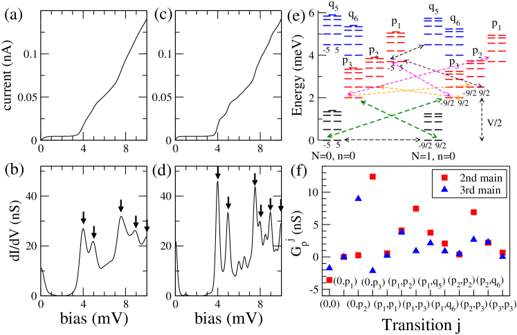
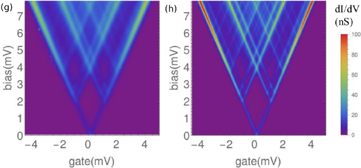
Figure 11: (Color Online) Calculated $I-V$ and $dI/dV$ vs $V$ at the charge degeneracy point for the case (ii) at 1.16 K [(a),(b)] and 0.58 K [(c),(d)]. The arrows in (d) point out the peaks ${\cal M}_{2}$, ${\cal M}_{3}$, ${\cal M}_{6}$, ${\cal M}_{7}$, ${\cal M}_{9}$, and ${\cal M}_{11}$ in Table 2. (e) Magnetic levels in the vibrational ground ($n=0$) and excited states $p_{1}$, $p_{2}$, $p_{3}$, $q_{5}$, and $q_{6}$ for the $N=0$ and $N=1$ states. The excited states are defined in Table 1. Some dominant tunneling pathways for the second peak at $V/2=2.0$ mV are indicated as the dashed arrows. Not all dominant pathways are drawn for clarity. (f) Contributions of different transitions $j$ to the second and third peaks. Calculated $dI/dV$ maps as a function of $V$ and $V_{g}$ for the case (ii) at 1.16 K (g) and 0.58 K (h).

Figures 11(a)-(d) exhibit the $I-V$ curve and $dI/dV$ vs $V$ for the case (ii) at the charge degeneracy point for 1.16 K and 0.58 K, respectively. In contrast to the case (i), we find that the current is significantly suppressed at a low bias, and that the $dI/dV$ peak at zero bias is considerably lower than the peaks arising from vibrational excitations marked by arrows in Figs. 11(b) and (d). Compare Fig. 11(d) with 5(d). This feature is found at both 1.16 K and 0.58 K. Henceforth, we consider the case at 0.58 K. The peaks from vibrational excitations occur at $V=$4.0, 5.0, 7.5, 8.0, 9.0, and 10.0 mV for $0\leq V\leq 10.0$ mV, which correspond to $2\hbar\omega_{1}$, $2\hbar\omega_{2}$, $2\hbar\omega_{3}$, $4\hbar\omega_{2}$, $2(\hbar\omega_{1}+\hbar\omega_{2})$, and $4\hbar\omega_{2}$, respectively. In general, peaks from vibrational excitations are found at $V=\sum_{i=1}^{3}2n_{i}\hbar\omega_{i}$, where $n_{1}+n_{2}+n_{3}=n>0$. All possible vibrational states for $n=0,1,2,3$ are listed in Table 1. Each of the peaks at $V=$4.0, 5.0, 7.5, 8.0, 9.0, and 10.0 mV dominantly originates from transitions between the vibrational ground state and a vibrational excited state, as shown in Table 2. Among the six peaks, the peak at $V=4.0$ mV has the largest height. In the bias range of interest, except for the zero-bias peak, four additional main peaks are identified at $V=$6.0, 6.5, 8.5, and 9.5 mV [Fig. 11(d)], each of which arises dominantly from transitions between a vibrational excited state to another vibrational excited state, as listed in Table 2. The heights of these peaks are smaller than those of the previous six peaks, because the vibrational excited states are poorly occupied. The stability diagrams shown in Figs. 11(g) and (h) also support the suppression of the low-bias current and its robustness with varying $V_{g}$ and $T$. The diagrams clearly reveal the peaks from the vibrational excitations parallel to the Coulomb diamond edges in the conduction region. Note that the values of $\lambda_{1,2,3}$ do not differ much from the value of $\lambda$ for the case (i), and that the ratio of the Franck-Condon factor for the peak at 4.0 mV to the factor at zero bias is the same for both cases, such as ${\cal F}_{\mathbf{0},p_{3}}/{\cal F}_{\mathbf{0},\mathbf{0}}={\cal F}_{0,1}/{\cal F}_{0,0}=\lambda^{2}=\lambda_{1}^{2}$. (Several values of the Franck-Condon factor for the case (ii) are listed in Table 4 in the Appendix.) Nonetheless, the case (ii) produces an effect similar to what was shown for a single mode with stronger electron-vibron coupling, referred to as the Franck-Condon blockade effect KOCH05 ; KOCH06 .

Table 1: List of all vibrational states $(n_{1},n_{2},n_{3})$ and their energies $E_{(n_{1},n_{2},n_{3})}$ (meV) for $n=0,1,2,3$, where $E_{(n_{1},n_{2},n_{3})}=\sum_{i=1}^{3}n_{i}\hbar\omega_{i}$.

label	$n_{1}$	$n_{2}$	$n_{3}$	$n$	$E_{(n_{1},n_{2},n_{3})}$	$2E_{(n_{1},n_{2},n_{3})}$
$\mathbf{0}$	0	0	0	0	0	0
$p_{1}$	0	0	1	1	3.75	7.5
$p_{2}$	0	1	0	1	2.5	5.0
$p_{3}$	1	0	0	1	2.0	4.0
$q_{1}$	0	0	2	2	7.5	15.0
$q_{2}$	0	1	1	2	6.25	12.5
$q_{3}$	0	2	0	2	5.0	10.0
$q_{4}$	1	0	1	2	5.75	11.5
$q_{5}$	1	1	0	2	4.5	9.0
$q_{6}$	2	0	0	2	4.0	8.0
$r_{1}$	0	0	3	3	11.25	22.5
$r_{2}$	0	1	2	3	10.0	20.0
$r_{3}$	0	2	1	3	8.75	17.5
$r_{4}$	0	3	0	3	7.5	15.0
$r_{5}$	1	0	2	3	9.5	19.0
$r_{6}$	1	1	1	3	8.25	16.5
$r_{7}$	1	2	0	3	7.0	14.0
$r_{8}$	2	0	1	3	7.75	15.5
$r_{9}$	2	1	0	3	6.5	13.0
$r_{10}$	3	0	0	3	6.0	12.0

Table 2: Eleven identified main $dI/dV$ peaks shown in Fig. 11(d) with the peak voltages $V_{p}$ (in meV) and the dominant transitions. The peak ${\cal M}_{11}$ at 10.0 mV arises from equally dominant two transitions $(p_{2},q_{1})$ and ($\mathbf{0}$,$q_{3}$). Here ($\mathbf{0},p_{3}$) represents all allowed transitions such as $\{|\psi^{N=0}_{M}\rangle\otimes|\mathbf{0}\rangle\leftrightarrow|\psi^{N=1}_{m}\rangle\otimes|p_{3}\rangle\}$ and $\{|\psi^{N=0}_{M}\rangle\otimes|p_{3}\rangle\leftrightarrow|\psi^{N=1}_{m}\rangle\otimes|\mathbf{0}\rangle\}$. Refer to Table 1 for the definitions of the vibrational states in the dominant transitions.

Label	${\cal M}_{1}$	${\cal M}_{2}$	${\cal M}_{3}$	${\cal M}_{4}^{\star}$	${\cal M}_{5}^{\star}$	${\cal M}_{6}$	${\cal M}_{7}$	${\cal M}_{8}^{\star}$	${\cal M}_{9}$	${\cal M}_{10}^{\star}$	${\cal M}_{11}$
$V_{p}$	0	4.0	5.0	6.0	6.5	7.5	8.0	8.5	9.0	9.5	10.0
Tran.	($\mathbf{0}$,$\mathbf{0}$)	($\mathbf{0}$,$p_{3}$)	($\mathbf{0}$,$p_{2}$)	($p_{3}$,$q_{3}$)	($p_{2}$,$q_{4}$)	($\mathbf{0}$,$p_{1}$)	($\mathbf{0}$,$q_{6}$)	($p_{3}$,$q_{2}$)	($\mathbf{0}$,$q_{5}$)	($q_{6}$,$r_{3}$)	($\mathbf{0}$,$q_{3}$)

To analyze the $dI/dV$ peak height, we separate contributions of different transitions $j$ to the first, second, and third main peaks (${\cal M}_{1}$, ${\cal M}_{2}$, ${\cal M}_{3}$) at 0, 4.0, and 5.0 mV. As shown in Fig. 11(f), at $V=4.0$ mV, the height of the peak ${\cal M}_{2}$ arising solely from transitions ($\mathbf{0}$,$\mathbf{0}$), ($\mathbf{0},p_{3}$), and ($p_{3}$,$p_{3}$), is about 9.5 nS, and this height is smaller than the height of the zero-bias peak ${\cal M}_{1}$ ($\sim$22 nS). The fact that the former height is smaller than the latter height, is similar to the case (i). However, interestingly, transitions ($p_{1}$,$p_{3}$), ($p_{2}$,$p_{3}$), ($p_{1}$,$p_{2}$), and ($p_{1}$,$q_{5}$) considerably contribute to the peak ${\cal M}_{2}$ with additional 22 nS, and so the total height of the peak ${\cal M}_{2}$ becomes larger than the height of the peak ${\cal M}_{1}$. This strikingly differs from the case (i) where the transitions ($n=1$,$n^{\prime}=1$) provide only a tiny increase of the height of the second peak (Fig. 5(f) in Sec.V.A). The key difference between the cases (i) and (ii) is that the latter has two additional modes whose energies are close to that of the lowest-energy mode. At $V/2=\hbar\omega_{1}$, the lowest levels $M=\pm 5$ or $m=\pm 9/2$ in the $p_{3}$ state are significantly occupied. Hence, for $(\hbar\omega_{2}-\hbar\omega_{1})<\hbar\omega_{1}$ and $(\hbar\omega_{3}-\hbar\omega_{1})<\hbar\omega_{1}$, the transitions ($p_{1}$,$p_{3}$) and ($p_{2}$,$p_{3}$) are also allowed [Fig. 11(e)]. Accordingly, the levels $M=\pm 5$ or $m=\pm 9/2$ in the $p_{2}$ and $p_{1}$ states are somewhat occupied, and so the transitions ($p_{1}$,$p_{2}$) and ($p_{1}$,$q_{5}$) are possible within the bias window. A similar analysis can be carried out for the third peak height. In this case, at $V=5.0$ mV, transitions ($\mathbf{0},p_{2}$) play a major role in the peak height, while transitions ($p_{1}$,$p_{2}$), ($p_{2}$,$p_{3}$), ($p_{2}$,$q_{6}$), and ($p_{1}$,$q_{5}$) provide considerable contributions to the height [Fig. 11(f)]. The overall height of the third peak turns out to be greater than the height of the zero-bias peak, although it is smaller than the second peak height. Similarly to the case (i), a satellite peak occurs at 1.0 mV and a flat shoulder appears on the left side of the second main peak [Fig. 11(d)], which is attributed to the magnetic anisotropy. The first (leftmost) satellite peak can be explained similarly to the case (i).

The Franck-Condon blockade effect has recently been observed in single-molecule transistors made of individual Fe₄ molecules BURZ14 , where the experimental data were fitted to vibrational excitations from a single normal mode of a non-magnetic molecule. The experimental values of $\lambda$ and $\hbar\omega$ were 2.0$\pm$0.2 and 2.3-2.6 meV, respectively BURZ14 , and they are in reasonable agreement with the corresponding DFT-calculated values. With the experimental level broadening $\Gamma\sim 1.0$ meV, the vibrational excitations may not be individually identified, and the calculated peaks at 4.0 mV and 5.0 mV could be viewed as a single peak in the experimental data.

V.4 Case (ii): Magnetic field dependence

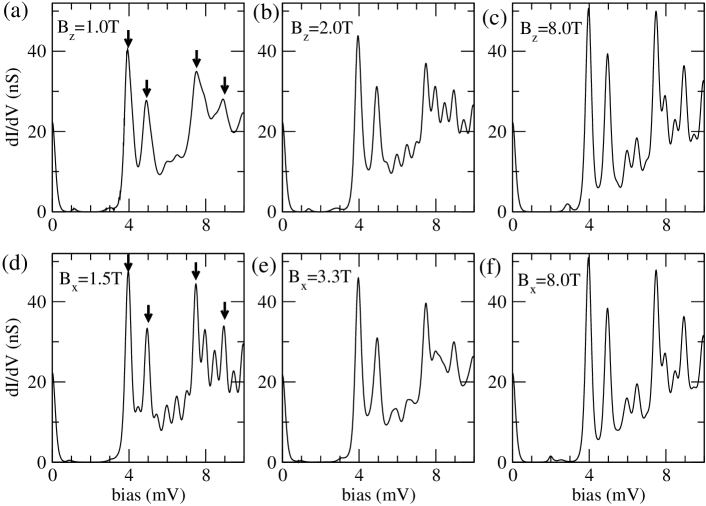
Figure 12: (a)-(c) $B_{z}$-field and (d)-(f) $B_{x}$-field dependence of $dI/dV$ vs $V$ in the case (ii) for the charge degeneracy point at 0.58 K. The arrows in (a) and (d) correspond to the peaks ${\cal M}_{2}$, ${\cal M}_{3}$, ${\cal M}_{6}$, and ${\cal M}_{9}$ in Table 2.

The heights of the main peaks and the heights and positions of the satellite peaks show strong $B$-field dependencies (Fig. 12), while the positions of the main peaks relative to the charge degeneracy point do not change with $B$ field, which is similar to the case (i). The main peaks from the tunneling between the levels in the $n=0$ state and the low-energy vibrational excited state, such as ${\cal M}_{2}$, ${\cal M}_{3}$, ${\cal M}_{6}$, and ${\cal M}_{9}$ (marked by the arrows in Fig. 12), have still a larger height than the zero-bias peak, independently of the orientation and magnitude of $B$ field. Some main peaks involved with either high-energy vibrational excited states or close to the other main peaks, are smeared out at some $B$ fields. For example, the three peaks ${\cal M}_{7}$, ${\cal M}_{8}^{\star}$, and ${\cal M}_{10}^{\star}$ used to appear at $V=$8.0, 8.5, and 9.5 mV in the absence of $B$ field, respectively, are not found at $B_{z}=1.0$ T [Fig. 12(a)]. In addition, the peaks ${\cal M}_{8}^{\star}$ and ${\cal M}_{10}^{\star}$ occurring at 8.5 and 9.5 mV for $B=0$, are not apparent for $B_{x}=3.3$ T, as shown in Fig. 12(e). In this section, we focus on the first, second, and third main peaks (${\cal M}_{1}$, ${\cal M}_{2}$, ${\cal M}_{3}$)and the satellite peaks between the first and second main peaks, in the presence of $B_{z}$ or $B_{x}$ field at 0.58 K for the charge degeneracy point. The height of the third main peak reveals a $B$-field dependence qualitatively different from that in the case (i). Note that the former peak dominantly arises from the tunneling between the levels in the $n=0$ state and in one of the $n=1$ states ($p_{2}$ state), while the latter peak mainly originates from the tunneling between the levels in the $n=0$ and $n=2$ states. Since some conductance features in the case (ii) are similar to those in the case (i), we underscore results distinctive from the case (i).

V.4.1 Main peaks

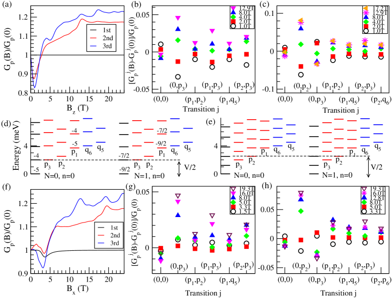
Figure 13: (Color online) (a) Ratio $G_{p}(B)/G_{p}(0)$ for the first (black), second (red), and third (blue) main peaks vs $B_{z}$ field for the case (ii) at 0.58 K. Normalized changes of contributions of different transitions $j$, $[G_{p}^{j}(B_{z})-G_{p}^{j}(0)]/G_{p}(0)$, for the second (b) and the third peaks (c) at different $B_{z}$ fields. Magnetic levels of the $n=0$, $p_{1}$, $p_{2}$, $p_{3}$, $q_{5}$, and $q_{6}$ states for the $N=0$ and $N=1$ states at $B_{z}=12.9$ T (d) and at $B_{x}=12.8$ T (e). Only the low-energy levels are shown to emphasize the low-energy region. The vertical arrow in (d) represents half of the bias voltage for the second peak with $B_{z}$ field, while the vertical arrow in (e) indicates half of the bias voltage for the third peak with $B_{x}$ field. (f) Ratio $G_{p}(B)/G_{p}(0)$ for the first, second, and third main peaks vs $B_{x}$ field for the case (ii) at 0.58 K. Changes of contributions of transitions $j$, $[G_{p}^{j}(B_{z})-G_{p}^{j}(0)]/G_{p}(0)$, at various $B_{x}$ fields for the second (g) and the third peaks (h).

As $B_{z}$ field increases, the heights of the second and third main peaks sharply decrease near 1.0 T, and then they rapidly rise well above the $G_{p}(B=0)$ values [Fig. 13(a)]. This is in contrast to the case (i), where the heights remain saturated to much lower values than the $G_{p}(0)$ values until about 12.0 T. Compare Fig. 13(a) with Fig. 8(a). To understand this difference, we examine $[G_{p}^{j}(B_{z})-G_{p}^{j}(0)]/G_{p}(0)$ for different transitions $j=(n,n^{\prime})$. At 1.0 T, similarly to the case (i), the abrupt drops of the heights of the peaks are due to the lift of the level degeneracy, which brings a large decrease of the dominant transitions ($\mathbf{0},p_{3}$) at $V=4.0$ mV and a large decrease of ($\mathbf{0},p_{2}$) for $V=5.0$ mV, as shown in Fig. 13(b) and (c). However, as $B_{z}$ field increases, the transitions ($\mathbf{0},p_{3}$) [($\mathbf{0},p_{2}$)] and other transitions begin to contribute more to the second (third) peak than at zero $B$ field, since new tunneling pathways are available from the three vibrational modes, compared to the case (i). More specifically, within $V=4.0$ mV, the transitions ($\mathbf{0},p_{3}$) and ($p_{2}$,$p_{3}$) participate in the tunneling more at 4.0 T than at zero $B$, while the transitions ($\mathbf{0},p_{3}$) and ($p_{1}$,$p_{3}$) involve more at 8.0 T than at 4.0 T. Within $V=5.0$ mV, the transitions ($\mathbf{0},p_{2}$) contribute to the third peak more at 4.0 T than at zero $B$, while the transitions ($\mathbf{0},p_{2}$), ($p_{1}$,$p_{2}$), and ($p_{2}$,$p_{3}$) participate in the peak more at 8.0 T than at 4.0 T.

The small bumps in the heights of the second and third peaks at $B_{z}=$12.9 T appear due to the same reason as in the case (i) (Sec.V.B.1). At this $B_{z}$ field, the spacing between the lowest and the first-excited levels for a given $N$ and $n$ state is comparable to $\hbar\omega_{1}$, such that the first-excited level in the $n=0$ state is degenerate with the lowest level in the $p_{3}$ state [Fig. 13(d)]. For $V=2\hbar\omega_{1}$, this noticeably increases the occupation of these two levels and the lowest level in the $n=0$ state, giving rise to an additional boost of the contributions of ($\mathbf{0},p_{3}$) and ($p_{1}$,$p_{3}$) to the second peak compared to lower $B_{z}$ fields. For $V=2\hbar\omega_{2}$, there is an increase of the occupation of the four levels in each charge state within the bias window, leading to an increase of the contributions of ($\mathbf{0},p_{2}$) and ($p_{2}$,$p_{3}$) to the third peak. Compare the peak height differences at 12.9 T with those at 8.0 T in Figs. 13(b) and (c). Another bump in the height of the third peak occurs at 17.2 T, where the spacing between the lowest and the first-excited levels for a given $N$ and $n$ state is now comparable to $\hbar\omega_{2}$, i.e., $(\hbar\omega_{2}/2-9D_{0})/g\mu_{B}=17.2$ T. In this case, the first-excited level in the $n=0$ state is degenerate with the lowest level in the $p_{2}$ state, which results in a slight increase of the transitions ($\mathbf{0},\mathbf{0}$) and ($p_{1}$,$q_{5}$), within $V=2\hbar\omega_{2}$, compared to lower $B_{z}$ fields (not shown). This produces a small bump in the third peak height at 17.2 K.

With a $B_{x}$ field, the third peak height shows an interesting feature, although the field dependence of the heights of the first and second main peaks is similar to that for the case (i). The height of the third main peak drops until 3.3 T, and as $B_{x}$ increases, it goes up with three apparent bumps at 12.8, 19.3, and 23.8 T, as shown in Fig. 13(f). At the first bump, the spacing between the second-excited level and the lowest level for a given $N$ and $n$ state is comparable to $\hbar\omega_{2}$, and so the second-excited level in the $n=0$ state is degenerate with the lowest level in the $p_{2}$ state [Fig. 13(e)]. For $V=2\hbar\omega_{2}$, this provides a substantial increase of the occupation of the levels within the bias window, leading to an increase of the transitions ($\mathbf{0},p_{2}$), ($p_{1}$,$p_{2}$) and ($p_{2}$,$p_{3}$), as indicated in Fig. 13(h). At the second bump, similarly to the case (i), the first-excited level in the $n=0$ state has the same energy as the lowest level in the $p_{3}$ state, giving rise to a slight increase of contributions of the transitions ($p_{2}$,$p_{3}$) to the third peak, compared to lower $B_{x}$ fields. At this $B_{x}$ field, a bump also appears in the height of the second peak [Fig. 13(g)], similarly to the case (i) (Sec.V.B.2). At the third bump, the first-excited level in the $n=0$ state is degenerate with the lowest level in the $p_{2}$ state. A slight increase of transitions ($\mathbf{0},\mathbf{0}$) brings the small bump in the third peak.

V.4.2 Satellite peaks

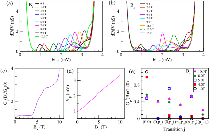
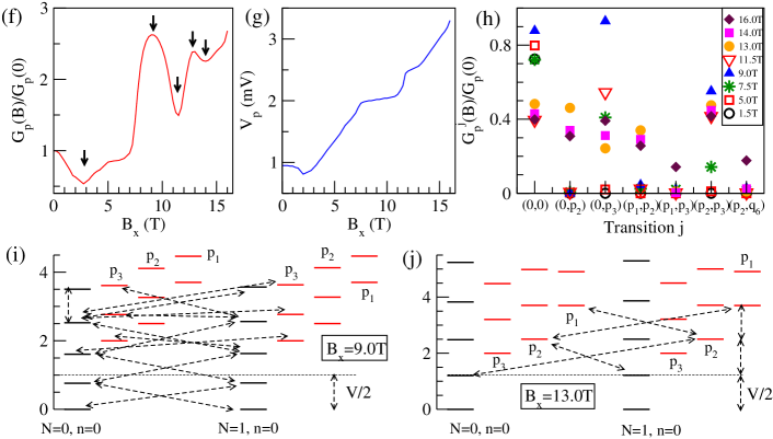
Figure 14: (Color online) (a) $B_{z}$-field and (b) $B_{x}$-field evolution of the satellite peaks for the case (ii) at 0.58 K. The height (c) and position (d) of the leftmost satellite peak vs $B_{z}$ field. (e) $G_{p}^{j}(B)/G_{p}(0)$ vs transitions $j$ for the leftmost satellite peak at various $B_{z}$ fields. The height (f) and position (g) of the leftmost satellite peak vs $B_{x}$ field. In (f), the arrows indicate the local minima and maxima in the height of the leftmost satellite peak. (h) $G_{p}^{j}(B)/G_{p}(0)$ vs transitions $j$ for the leftmost satellite peak at various $B_{x}$ fields. Dominant tunneling pathways for the leftmost satellite peak at $B_{x}$=9.0 T (i) and 13.0 T (j), where the vertical arrows indicate half of the peak bias. Only low-energy magnetic levels are shown to emphasize the transitions in the low-energy region.

We first discuss the case of $B_{z}$ field. Figure 14(a) shows how the satellite peaks between the first and second main peaks evolve with $B_{z}$ field. Compare Figs. 14(a),(c),(d) with Figs. 10(a),(c),(d). Similarly to the case (i), near 4.5 T, the leftmost satellite peak merges with the second satellite peak, and the merged satellite peak has a large height which is strongly deviated from the case of without electron-vibron coupling. We find that at 5.0 T, the transitions ($\mathbf{0}$,$p_{3}$) and ($p_{2}$,$p_{3}$) contribute to the first satellite peak as much as the transitions ($\mathbf{0}$,$\mathbf{0}$) [Fig. 14(e)]. The energy difference between the lowest levels in the $p_{3}$ and $p_{2}$ states is only 0.5 meV, and the low-lying levels in the $p_{3}$ state are occupied from the transitions ($\mathbf{0}$,$p_{3}$). Thus, the transitions ($p_{2}$,$p_{3}$) can participate in the tunneling for a bias window of 2.2 mV at 5.0 T. As $B_{z}$ field further increases, more diverse types of transitions contribute to the merged satellite peak. Interestingly, the contributions of the transitions ($p_{1}$,$p_{3}$) to the merged satellite peak are negligible, because the energy difference between the lowest levels in the $p_{3}$ and $p_{1}$ states exceeds a half of the peak bias voltage. The transitions ($p_{1}$,$q_{5}$) do not contribute to the satellite peak despite the small energy difference between the lowest levels in the $p_{1}$ and $q_{5}$ state because the levels in the $p_{1}$ state are not occupied. The merged peak height increases to a much higher value than the case (i), although the peak position is the same as that for the case (i). The merged satellite peak eventually disappears above 10.0 T at 0.58 K, attributed to the same reason as in the case (i) (Sec.V.B.3).

With a $B_{x}$ field, below 7.0 T, the evolution of the satellite peaks [Fig. 14(b)] is similar to the case (i) (Sec.V.B.4). As $B_{x}$ field increases, the leftmost satellite peak is shifted toward a higher bias, while the second satellite peak moves toward a lower bias. Interestingly, around 7.0 T, three satellite peaks appear instead of two, while around 9.0 T, the first two satellite peaks become merged but the third peak still survives [Fig. 14(b)]. Then at 13.0 T, the survived two satellite peaks are completely merged. The merged peak is shifted toward a higher bias at higher $B$ fields. Compare Fig. 14(b) with Fig. 10(b) at 7.0 T and 9.0 T. Comparing with the case (i), the leftmost peak height does not drop to the $G_{p}(0)$ value above 11.5 T. Instead it resumes to grow and reaches to a local maximum at 13.0 T. Then the height undergoes a slight decrease with another upturn until the merged peak disappears above 16.0 T [Fig. 14(f)]. At the $B_{x}$ fields where the height of the leftmost satellite peak reaches to local maxima, the peak position remains almost flat [Fig. 14(g)].

Above $B_{x}=$7.0 T, the vibrational excited states play an important role even in the satellite peaks. At 7.5 T, the transitions ($\mathbf{0}$,$p_{3}$) contribute substantially to the leftmost satellite peak, while at 9.0 T (at the maximum peak height), there is a great increase of the transitions ($\mathbf{0}$,$p_{3}$) and ($p_{2}$,$p_{3}$) compared to lower $B_{x}$ fields [Fig. 14(h)]. The peak bias at 9.0 T is still higher than twice the energy difference between the lowest levels in the $n=0$ state. The level spacing is larger for higher levels. Some dominant transition pathways within ($\mathbf{0}$,$p_{3}$) are shown in Fig. 14(i). The transitions ($\mathbf{0}$,$\mathbf{0}$) allow the intermediate-energy levels of the $n=0$ state to be occupied, and the transitions ($\mathbf{0}$,$p_{3}$) occur between these levels and the low-lying levels in the $p_{3}$ state. Now the occupation in the $p_{3}$ state induces the transitions ($p_{2}$,$p_{3}$). As $B_{x}$ increases to 11.5 T, the transitions ($\mathbf{0}$,$p_{3}$) and ($p_{2}$,$p_{3}$) greatly decrease, which gives rise to a drop in the peak height [Fig. 14(f),(h)]. As discussed in the case (i), above 11.5 T, the peak bias is determined by the spacing between the two lowest levels in the $n=0$ state. At 13.0 T (at the local maximum height), the spacing between the lowest and the first-excited level in the $n=0$ state is comparable to the energy difference between the first-excited level in the $n=0$ state and the lowest-level in the $p_{2}$ state [vertical arrows in Fig. 14(j)]. Thus, at this $B$ field, the transitions ($\mathbf{0}$,$p_{2}$) increase and they contribute to the satellite peak height. Moreover, the level spacing in the $n=0$ state is comparable to the energy difference between the lowest levels in the $p_{2}$ and $p_{1}$ state. Since the lowest level in the $p_{2}$ state is occupied, the transitions ($p_{1}$,$p_{2}$) also contribute to the peak height at this $B$ field. Dominant transition pathways among ($\mathbf{0}$,$p_{2}$) and ($p_{1}$,$p_{2}$) are shown in Fig. 14(j). With a higher $B_{x}$ field, other transitions requiring higher energies participate in the tunneling. The merged satellite peak disappears above 16.0 T.

VI Conclusion

We have shown that magnetic anisotropy provides new features concerning electron-vibron coupling in electron transport through single anisotropic molecules such as the SMM Fe₄. The heights of the vibrational conductance peaks show an unusual $B$-field dependence at low temperatures. When the current flows via the vibrational excited states of the Fe₄, the magnetic levels in the vibrational ground and excited states participate in the tunneling. The separation between the magnetic levels strongly depends on the direction and magnitude of applied $B$-field, and so the occupation of the levels and transition rates between them are accordingly modified with $B$ field. As a result, the vibrational conductance peaks are highly influenced by the direction as well as magnitude of the applied $B$ field. Interestingly, when the two lowest levels in the $n=0$ state are separated by about the vibrational energies at high $B$ fields, a sudden large jump in the peak height is expected. Moreover, the magnetic anisotropy introduces satellite conductance peaks whose position and height are varied with the direction and magnitude of the applied $B$ field. At zero $B$ field, the low-bias satellite peak originates from the current via the magnetic levels in the vibrational ground states only, while at intermediate $B$ fields, the levels in the vibrational first-excited state start to contribute to the satellite peak. Another interesting point is the effect of multiple strong electron-vibron coupled modes whose energies are close to one another. For such multiple modes the vibrational conductance peaks are greatly enhanced compared to a single mode with the similar electron-vibron coupling. Our findings may be extended to studies of spin-vibron coupling effects, higher-order tunneling processes, and many-spin model Hamiltonian in transport via individual anisotropic molecules. For comparison with experiment, caution has to be exercised in two aspects such as level broadening and excited spin multiplets. An experimental level broadening may correspond to a sum of the broadenings of several magnetic levels rather than the broadening of one level. In the case of without electron-vibron coupling, numerical renormalization group studies show that main transport properties are not affected by consideration of a larger level broadening MISI14 . Very high external $B$ fields could induce some overlap with the low-lying levels of the excited spin multiplet(s) in each charge state.

*

Appendix A Franck-Condon factors for several transitions in the cases (i) and (ii).

The Franck-Condon factors for several transitions are computing for the cases (i) and (ii), by applying the recursion relations RUHO94 ; RUHO00 to the overlap matrices (Sec.IV.B).

Table 3: Franck-Condon factors for several transitions $(n,n^{\prime})$ for the case (i).

$(n,n^{\prime})$	${\cal F}_{n,n^{\prime}}$
$(0,0)$	0.199
$(0,1)$	0.321
$(0,2)$	0.259
$(0,3)$	0.139
$(1,1)$	0.075
$(1,2)$	0.024
$(1,3)$	0.166
$(2,2)$	0.171
$(2,3)$	0.031
$(3,3)$	0.081

Table 4: Franck-Condon factors for several transitions $(n,n^{\prime})$ for the case (ii).

$(n,n^{\prime})$	${\cal F}_{n,n^{\prime}}$
(${\mathbf{0}}$,${\mathbf{0}}$)	0.00403
(${\mathbf{0}}$,$p_{1}$)	0.00860
(${\mathbf{0}}$,$p_{2}$)	0.00713
(${\mathbf{0}}$,$p_{3}$)	0.00650
($p_{1}$,$p_{1}$)	0.00516
($p_{1}$,$p_{2}$)	0.0152
($p_{1}$,$p_{3}$)	0.0139
($p_{1}$,$q_{5}$)	0.0245
($p_{1}$,$q_{6}$)	0.0112
($p_{2}$,$p_{2}$)	0.00238
($p_{2}$,$p_{3}$)	0.0115
($p_{2}$,$q_{5}$)	0.00385
($p_{2}$,$q_{6}$)	0.00928
($p_{3}$,$p_{3}$)	0.00151
($p_{3}$,$q_{5}$)	0.00268
($p_{3}$,$q_{6}$)	0.000487

References

- (1) J. R. Friedman, M. P. Sarachik, J. Tejada, and R. Ziolo, Phys. Rev. Lett. 76, 3830 (1996).
- (2) L. Thomas, F. Lionti, R. Ballou, D. Gatteschi, R. Sessoli, and B. Barbara, Nature 383, 145 (1996).
- (3) E. M. Chudnovsky and J. Tejada, Macroscopic Quantum Tunneling of the Magnetic Moment, Cambridge Studies in Magnetism Vol. 4 (Cambridge University Press, Cambridge, 1998).
- (4) W. Wernsdorfer and R. Sessoli, Science 284, 133 (1999).
- (5) A. Garg, Europhys. Lett. 22, 205 (1993).
- (6) E. Burzuri, F. Luis, O. Montero, B. Babara, R. Ballou, and S. Maegawa, Phys. Rev. Lett. 111, 057201 (2013).
- (7) H. B. Heersche, Z. de Groot, J. A. Folk, H. S. van der Zant, C. Romeike, M. R. Wegewijs, L. Zobbi, D. Barreca, E. Tondello, and A. Cornia, Phys. Rev. Lett. 96, 206801 (2006).
- (8) M. N. Leuenberger and E. R. Mucciolo, Phys. Rev. Lett. 97, 126601 (2006).
- (9) C. Romeike, M. R. Wegewijs, and H. Schoeller, Phys. Rev. Lett. 96, 196805 (2006).
- (10) C. Timm and F. Elste, Phys. Rev. B 73, 235304 (2006).
- (11) M.-H. Jo, J. E. Grose, K. Baheti, M. M. Deshmukh, J. J. Sokol, E. M. Rumberger, D. N. Hendrickson, J. R. Long, H. Park, and D. C. Ralph, Nano Lett. 6, 2014-2020 (2006).
- (12) S. Barraza-Lopez, K. Park, V. García-Suárez, and J. Ferrer, Phys. Rev. Lett. 102, 246801 (2009).
- (13) A. S. Zyazin, J. W. G. van den Berg, E. A. Osorio, H. S. J. van der Zant, N. P. Konstantinidis, M. Leijnse, M. R. Wegewijs, F. May, W. Hofstetter, C. Danieli, and A. Cornia, Nano Lett. 10, 3307-3311 (2010).
- (14) D. A. Garanin and E. Chudnovsky, Phys. Rev. X 1, 011005 (2011).
- (15) C. Timm and M. Di Ventra, Phys. Rev. B 86, 104427 (2012).
- (16) M. Ganzhorn, S. Klyatskaya, M. Ruben, and W. Wernsdorfer, Nat. Nanotech. 8, 165 (2013).
- (17) M. Misiorny and J. Barnaś, Phys. Rev. Lett. 111, 046603 (2013).
- (18) Y.-N. Wu, X.-G. Zhang, and H.-P. Cheng, Phys. Rev. Lett. 110, 217205 (2013).
- (19) J. I. Romero and E. R. Mucciolo, J. Phys.: Condens. Matter 26, 195301 (2014).
- (20) B. J. LeRoy, S. G. Lemay, K. Kong, and C. Dekker, Nature 432, 371 (2004).
- (21) S. Sapmaz, P. Jaillo-Herrero, Ya. M. Blanter, C. Dekker, and H. S. J. van der Zant, Phys. Rev. Lett. 96, 026801 (2006).
- (22) R. Leturcq, C. Stampfer, K. Inderbitzin, L. Durrer, C. Hierold, E. Mariani, M. G. Schultz, F. von Oppen, and K. Ensslin, Nat. Phys. 5, 327 (2009).
- (23) A. Benyamini, A. Hamo, S. Viola Kusminskiy, F. von Oppen, and S. Ilani, Nat. Phys. 10, 151 (2014).
- (24) B. C. Stipe, M. A. Rezaei, and W. Ho, Science 280, 1732 (1998).
- (25) H. Park, J. Park, A. K. L. Lim, E. H. Anderson, A. P. Alivisatos, and P. L. McEuen, Nature 407, 57 (2000).
- (26) L. H. Yu, Z. K. Keane, J. W. Ciszek, L. Cheng, M. P. Stewart, J. M. Tour, and D. Natelson, Phys. Rev. Lett. 93, 266802 (2004).
- (27) N. P. de Leon, W. Liang, Q. Gu, and H. Park, Nano Lett. 8, 2963 (2008).
- (28) E. Burzuri, Y. Yamamoto, M. Warnock, X. Zhong, K. Park, A. Cornia, and H. S. J. van der Zant, Nano Lett. 14, 3191 (2014).
- (29) J. Koch and F. von Oppen, Phys. Rev. Lett. 94, 206804 (2005).
- (30) J. Koch, F. von Oppen, and A. V. Andreev, Phys. Rev. B 74, 205438 (2006).
- (31) A. Mitra, I. Aleiner, and A. J. Millis, Phys. Rev. B 69, 245302 (2004).
- (32) M. Galperin, M. A. Ratner, and A. Nitzan, J. Phys.: Cond. Matt. 19, 103201 (2007).
- (33) D. Secker, S. Wagner, S. Ballmann, R. Härtle, M. Thoss, and H. B. Weber, Phys. Rev. Lett. 106, 136807 (2011).
- (34) R. Härtle, M. Butzin, and M. Thoss, Phys. Rev. B 87, 085422 (2013).
- (35) P. S. Cornaglia, G. Usaj, and C. A. Balseiro, Phys. Rev. B 76, 241403(R) (2007).
- (36) T. Frederiksen, M. Paulsson, M. Brandbyge, and A.-P. Jauho, Phys. Rev. 75, 205413 (2007).
- (37) M. Paulsson, T. Frederiksen, and M. Brandbyge, Phys. Rev. B 72, 201101(R) (2005).
- (38) K. D. McCarthy, N. Prokof’ev, and M. T. Tuominen, Phys. Rev. B 67, 245415 (2003).
- (39) J. S. Seldenthuis, H. S. J. van der Zant, M. A. Ratner, and J. M. Thijssen, ACS Nano 2, 1445 (2008).
- (40) E. Burzuri, A. S. Zyazin, A. Cornia, and H. S. J. van der Zant, Phys. Rev. Lett. 109, 147203 (2012).
- (41) S. Accorsi, A.-L. Barra, A. Caneschi, G. Chastanet, A. Cornia, A. C. Febretti, D. Gatteschi, C. Mortaló, E. Olivieri, F. Parenti, P. Rosa, R. Sessoli, L. Sorace, W. Wernsdorfer, and L. Zobbi, J. Am. Chem. Soc. 128 4742-4755 (2006).
- (42) M. R. Pederson and K. A. Jackson, Phy. Rev. B 41, 7453 (1990); K. A. Jackson and M. R. Pederson, ibid. 42, 3276 (1990); D. V. Porezag, Ph.D. thesis, Chemnitz Technical Institute, 1997; D. Porezag and M. R. Pederson, Phys. Rev. A 60, 2840 (1999).
- (43) J. P. Perdew, K. Burke, and M. Ernzerhof, Phys. Rev. Lett. 77, 3865 (1996).
- (44) H. H. Liu, S. H. Lin, and N. T. Yu, Biophys. J. 57, 851 (1990).
- (45) M. R. Pederson and S. N. Khana, Phys. Rev. B 60, 9566 (1999).
- (46) J. F. Nossa, M. F. Islam, C. M. Canali, and M. R. Pederson, Phys. Rev. B 88, 224423 (2013).
- (47) M. R. Pederson, R. A. Heaton, C. C. Lin, J. Chem. Phys. 82, 2688 (1985).
- (48) D. Porezag and M. R. Pederson, Phys. Rev. B 54, 7830 (1996).
- (49) L. Bogani, C. Danieli, E. Biavardi, N. Bendiab, A.-L. Barra, E. Dalcanale, W. Wernsdorfer, and A. Cornia, Angew. Chem. Int. Ed. 48, 746 (2009).
- (50) J. S. Seldenthuis, Ph.D. thesis, T.U. Delft, Netherlands, 2011.
- (51) P. T. Ruhoff, Chem. Phys. 186, 355 (1994).
- (52) P. T. Ruhoff and M. A. Ratner, Int. J. Quan. Chem. 77, 383 (2000).
- (53) H. A. van der Vorst, SIAM J. Sci. Stat. Comput. 13, 631 (1992).
- (54) M. Misiorny, E. Burzuri, R. Gaudenzi, K. Park, M. Leijnse, M. R. Wegewijs, J. Paaske, A. Cornia, and H. S. J. van der Zant, arXiv:1407.5265 (unpublished).