Abstract

We present the Bayesian Echo Chamber, a new Bayesian generative model for social interaction data. By modeling the evolution of people’s language usage over time, this model discovers latent influence relationships between them. Unlike previous work on inferring influence, which has primarily focused on simple temporal dynamics evidenced via turn-taking behavior, our model captures more nuanced influence relationships, evidenced via linguistic accommodation patterns in interaction content. The model, which is based on a discrete analog of the multivariate Hawkes process, permits a fully Bayesian inference algorithm. We validate our model’s ability to discover latent influence patterns using transcripts of arguments heard by the US Supreme Court and the movie “12 Angry Men.” We showcase our model’s capabilities by using it to infer latent influence patterns from Federal Open Market Committee meeting transcripts, demonstrating state-of-the-art performance at uncovering social dynamics in group discussions.

1 INTRODUCTION

As increasing quantities of social interaction data become available, often through online sources, researchers strive to find new ways of using these data to learn about human behavior. Most social processes, in which people or groups of people interact with one another in order to achieve specific (and sometimes contradictory) goals, are extremely complex. In order to construct realistic models of these social processes, it is therefore necessary to take into account their structure (e.g., who spoke with whom), content (e.g., what was said), and temporal dynamics (e.g., when they spoke).

When studying social processes, one of the most pervasive questions is “who influences whom?” This question is of interest not only to sociologists and psychologists, but also to political scientists, organizational scientists, and marketing researchers. Since influence relationships are seldom made explicit, they must be inferred from other information. Influence has traditionally been studied by analyzing declared structural links in observed networks, such as Facebook “friendships” [Backstrom et al.,, 2006], paper citations [de Solla Price,, 1965], and bill co-sponsorships [Fowler,, 2006]. For many domains, however, explicitly stated links do not exist, are unreliable, or fail to reflect pertinent behavior. In these domains, researchers have used observed interaction dynamics as a proxy by which to infer influence and other social relationships. Much of this work has concentrated (either implicitly or explicitly) on turn-taking behavior—i.e., “who acts next.”

In this paper, we take a different approach: we move beyond turn-taking behavior, and present a new model, the Bayesian Echo Chamber, that uses observed interaction content, in the context of temporal dynamics, to capture influence. Our model draws upon a substantial body of work within sociolinguistics indicating that when two people interact, either orally or in writing, the use of a word by one person can increase the other person’s probability of subsequently using that word. Furthermore, the extent of this increase depends on power differences and influence relationships: the language used by a less powerful person will drift further so as to more closely resemble or “accommodate” the language used by more powerful people. This phenomenon is known as linguistic accommodation [West and Turner,, 2010]. We demonstrate that linguistic accommodation can reveal more nuanced influence patterns than those revealed by simple reciprocal behaviors such as turn-taking.

The Bayesian Echo Chamber is a new, mutually exciting, dynamic language model that combines ideas from Hawkes processes [Hawkes,, 1971] with ideas from Bayesian language modeling. We draw inspiration from Blundell et al.’s model of turn-taking behavior [2012] (described in section 2) to define a new model of the mutual excitation of words in social interactions. This approach, which leverages a discrete analog of a multivariate Hawkes process, enables the Bayesian Echo Chamber to capture linguistic accommodation patterns via latent influence variables. These variables define a weighted influence network that reveals fine-grained information about who influences whom.

We provide details of the Bayesian Echo Chamber in section 3, including an MCMC algorithm for inferring the latent influence variables (and other parameters) from real-world data. To validate this algorithm, we provide parameter recovery results obtained using synthetic data. In section 5 we compare to several baseline models on data sets including arguments heard by the US Supreme Court [MacWhinney,, 2007] and the transcript of the 1957 movie “12 Angry Men.” We compare influence networks inferred using our model to those inferred using Blundell et al.’s model. We show that by focusing on linguistic accommodation patterns, our model infers different—more substantively meaningful—influence networks than those inferred from turn-taking behavior. We also combine our model with Blundell et al.’s so as to jointly model turn-taking and linguistic accommodation. We investigate the possibility of tying the latent influence parameters to see if a single global notion of influence can be discovered. Finally, we showcase our model’s potential as an exploratory analysis tool for social scientists using recently released transcripts of Federal Reserve’s Federal Open Market Committee meetings.

2 INFLUENCE VIA TURN-TAKING

In this section, we give a brief description of a variant of Blundell et al.’s model for inferring influence from turn-taking behavior. Unlike Blundell et al.’s original paper, which modeled pairwise actions, we concentrate on a broadcast or group discussion setting appropriate for the data that we wish to model. (We also do not cluster participants by their interaction patterns.) This setting, in which every utterance is heard by and thus potentially influences every participant, occurs in many scenarios of interest to social scientists. Furthermore, the comparatively information-impoverished nature of this setting makes it one in which ability to infer influence relationships is deemed extremely valuable.

Blundell et al.’s model specifies a probabilistic generative process for the time stamps $\mathcal{T}=\{\mathcal{T}^{(p)}\}_{p=1}^{P}$ associated with a set of actions made by $P$ people. In a group discussion setting, these actions correspond to utterances, and the model captures who will speak next and when that next utterance will occur. Letting $N^{(p)}(T)$ denote the total number of utterances made by person $p$ over the entire observation interval $[0,T)$, each utterance made by $p$ is associated with a time stamp indicating its start time, i.e., $\mathcal{T}^{(p)}=\{t_{n}^{(p)}\}_{n=1}^{N^{(p)}(T)}$. We assume that the duration of each utterance $\Delta t_{n}^{(p)}$ is observed and that its end time ${t^{\prime}}^{(p)}_{n}$ can be calculated from its start time and duration: ${t^{\prime}}^{(p)}_{n}=t^{(p)}_{n}+\Delta t_{n}^{(p)}$.

Hawkes processes [Hawkes,, 1971]—a class of self- and mutually exciting doubly stochastic point processes—form the mathematical foundation of Blundell et al.’s model. A Hawkes process is a particular form of inhomogeneous Poisson process with a conditional stochastic rate function $\lambda(t)$ that depends on the time stamps of all events prior to time $t$. Blundell et al. model turn-taking interactions using coupled Hawkes processes. For a group discussion setting, we instead define a multivariate Hawkes process, in which each person $p$ is associated with his or her own Hawkes process defined on $(0,\infty)$. Letting $N^{(p)}(\cdot)$ denote the counting measure of person $p$’s Hawkes process, which takes as its argument an interval $[a,b)$ and returns the number of utterances made by $p$ during that interval, the stochastic rate function for $p$’s Hawkes process is

$$\lambda^{(p)}(t) =\lambda_{0}^{(p)}+\sum_{q\neq p}\int_{0}^{t^{-}}g^{(qp)}(t,u)\,\textrm{d}N^{(q)}(u)$$ (1)

$$=\lambda_{0}^{(p)}+\sum_{q\neq p}\sum_{n:{t^{\prime}}_{n}^{(q)}<t}g^{(qp)}(t,{t^{\prime}}^{(q)}_{n}),$$ (2)

where $\lambda_{0}^{(p)}$ is person $p$’s base rate of utterances and $g(t,u)$ is a non-negative stationary kernel function that specifies the extent to which an event at time $u<t$ increases the instantaneous rate at time $t$, as well as the way in which this increase decays over time. Person $p$’s rate function is coupled with the Hawkes processes of the other $P-1$ people via their respective counting measures $\{N^{(q)}(\cdot)\}_{q\neq p}$ and the kernel function $g(t,u)$. Note that time stamp ${t^{\prime}}_{n}^{(q)}$ is the end time of the $n^{\textrm{th}}$ utterance made by person $q$. Consequently, an utterance made by person $q$ only causes an increase in $p$’s instantaneous rate after $q$’s utterance is complete.

Blundell et al. use a standard exponential kernel function of the form $g^{(qp)}(t,u)=\nu^{(qp)}\exp{\left(-(t-u)\,/\,\tau_{T}^{(p)}\right)}$, although the shape of the non-negative kernel function $g^{(qp)}(t,u)$ could instead be learned in a non-parametric fashion [Zhou et al.,, 2013] if desired. Non-negative parameter $\nu^{(qp)}$ controls the degree of instantaneous excitation from person $q$ to person $p$, while $\tau_{T}^{(p)}$ is a time decay parameter specific to person $p$ that characterizes how fast excitation decays. Since the goal is to model influence between people, self-excitation is prohibited by enforcing $\nu^{(pp)}=0$. Since a larger value of $\nu^{(qp)}$ will result in a higher instantaneous rate of utterances for person $p$, the non-negative parameters $\{\{\nu^{(qp)}\}_{q\neq p}\}_{p=1}^{P}$ define a weighted influence network that reflects conversational turn-taking behavior—i.e., who is likely to speak next and when that next utterance will occur. Details of an inference algorithm and appropriate priors for this turn-taking-based model can be found in the supplementary material.

3 INFLUENCE VIA LINGUISTIC ACCOMMODATION

In this section, we present our new dynamic Bayesian language model, the Bayesian Echo Chamber. This model specifies a probabilistic generative process for the words that occur in a set of utterances $\{\mathcal{W}^{(p)}\}_{p=1}^{P}$ made by $P$ people, conditioned on the utterance start times and durations. Letting $N^{(p)}(T)$ denote the total number of utterances made by person $p$ over the interval $[0,T)$, each utterance made by $p$ consists of $L_{n}^{(p)}$ word tokens, i.e., $\mathcal{W}^{(p)}=\{\{w_{l,n}^{(p)}\}_{l=1}^{L_{n}^{(p)}}\}_{n=1}^{N^{(p)}(T)}$. Each token is an instance of one of $V$ unique word types.

The generative process for each token draws upon ideas from both dynamic Bayesian language modeling and multivariate Hawkes processes. The $l^{\textrm{th}}$ token in the $n^{\textrm{th}}$ utterance made by person $p$ is drawn from categorical distribution specific to that utterance: $w_{l,n}^{(p)}\sim\textrm{Categorical}\,(\bm{\phi}_{n}^{(p)})$, where $\bm{\phi}_{n}^{(p)}$ is a $V$-dimensional discrete probability vector. Each such probability vector is in turn drawn from a Dirichlet distribution with a person-specific concentration (or precision) parameter and an utterance-specific base measure: $\bm{\phi}_{n}^{(p)}\sim\text{Dirichlet}\,(\alpha^{(p)},\bm{B}_{n}^{(p)})$. Concentration parameter $\alpha^{(p)}$ is a positive scalar that determines the variance of the distribution, while base measure $\bm{B}_{n}^{(p)}$ is a $V$-dimensional discrete probability vector that specifies the mean of the distribution and satisfies

$$B^{(p)}_{v,n}\propto\beta^{(p)}_{v}+\sum_{q\neq p}\rho^{(qp)}\psi^{(qp)}_{v,n}\ \textrm{and}\ \sum_{v=1}^{V}B_{v,n}^{(p)}=1.$$ (3)

$V$-dimensional vector $\bm{\beta}^{(p)}\in\mathbb{R}_{+}^{V}$ characterizes person $p$’s inherent language usage. Non-negative parameter $\rho^{(qp)}$ controls the degree of linguistic excitation from person $q$ to person $p$. Self-excitation is prohibited by enforcing $\rho^{(pp)}=0$. Finally, $\bm{\psi}^{(qp)}_{n}\in\mathbb{R}_{+}^{V}$ is a $V$-dimensional vector of decayed excitation pseudocounts, constructed from all utterances made by person $q$ prior to person $p$’s $n^{\textrm{th}}$ utterance, satisfying

$$\psi^{(qp)}_{v,n} =\sum_{m:{t^{\prime}}^{(q)}_{m}<t^{(p)}_{n}}\left(\sum_{l=1}^{L_{m}^{(q)}}\mathbf{1}(w_{l,m}^{(q)}=v)\right)\times{}$$

$$\quad\quad\exp{\left(-\frac{t_{n}^{(p)}-{t^{\prime}}_{m}^{(q)}}{\tau_{L}^{(p)}}\right)},$$ (4)

where $\mathbf{1}(\cdot)$ is the indicator function. The inner sum is therefore equal to the number of tokens of type $v$ in person $q$’s $m^{\textrm{th}}$ utterance. Note that ${t^{\prime}}_{m}^{(q)}$ is the end time of that utterance. Consequently, an utterance made by $q$ only affects $\bm{\psi}^{(qp)}$, and hence base measure $\bm{B}_{n}^{(p)}$, after $q$’s utterance is complete. Finally, $\tau_{L}^{(p)}$ is a time decay parameter specific to person $p$ that characterizes how fast excitation decays. Since a larger value of $\rho^{(qp)}$ will increase the probability of person $p$ using word types previously used by person $q$, the parameters $\{\{\rho^{(qp)}\}_{q\neq p}\}_{p=1}^{P}$ define a weighted influence network that reflects linguistic accommodation. A graphical model depicting the dependencies between utterances is in the supplementary material.

3.1 Inference

For real-world group discussions, the utterance contents $\mathcal{W}=\{\mathcal{W}^{(p)}\}_{p=1}^{P}$, start times $\mathcal{T}$, and durations ${\mathcal{D}}$ are observed, while parameters $\Theta=\{\{\bm{\phi}_{n}^{(p)}\}_{n=1}^{N^{(p)}(T)},\alpha^{(p)},\bm{\beta}^{(p)},\{\rho^{(qp)}\}_{q\neq p},\tau_{L}^{(p)}\}_{p=1}^{P}$ are unobserved; however, information about the values of these unobserved parameters can be quantified via their posterior distribution given $\mathcal{W}$, $\mathcal{T}$, and $\mathcal{D}$, i.e., $P(\Theta\,|\,\mathcal{W},\mathcal{T},\mathcal{D})\propto P(\mathcal{W}\,|\,\Theta,\mathcal{T},\mathcal{D})\,P(\Theta)$. The likelihood term can be factorized into the following product due to our model’s independence assumptions:

$$P(\mathcal{W}\,|\,\Theta,\mathcal{T},\mathcal{D})=$$

$$\quad\prod_{p=1}^{P}\prod_{n=1}^{N^{(p)}(T)}P(\bm{w}_{n}^{(p)}\,|\,\{\{\bm{w}_{m}^{(q)}\}_{m:{t^{\prime}}_{m}^{(q)}<t^{(p)}_{n}}\}_{q\neq p},\Theta).$$

Using Dirichlet–multinomial conjugacy, the probability vectors $\{\{\bm{\phi}_{n}^{(p)}\}_{n=1}^{N^{(p)}(T)}\}_{p=1}^{P}$ can be integrated out:

$$P(\mathcal{W}\,|\,\Theta,\mathcal{T},\mathcal{D})=$$

$$\quad\quad\prod_{p=1}^{P}\prod_{n=1}^{N^{(p)}}\prod_{l=1}^{L^{(p)}_{n}}\frac{\sum_{l^{\prime}=1}^{l-1}\mathbf{1}(w_{l^{\prime},n}^{(p)}=w_{l,n}^{(p)})+\alpha^{(p)}B^{(p)}_{w^{(p)}_{l,n},n}}{l-1+\alpha^{(p)}}.$$

To complete the specification of $P(\Theta)$, we place gamma priors over the remaining parameters $\{\alpha^{(p)},\bm{\beta}^{(p)},\{\rho^{(qp)}\}_{q\neq p},\tau_{L}^{(p)}\}_{p=1}^{P}$. The resultant posterior distribution $P(\Theta\,|\,\mathcal{W},\mathcal{T},\mathcal{D})$ is analytically intractable; however, posterior samples of $\{\alpha^{(p)},\bm{\beta}^{(p)},\{\rho^{(qp)}\}_{q\neq p},\tau_{L}^{(p)}\}_{p=1}^{P}$ can be obtained using a collapsed slice-within-Gibbs sampling algorithm [Neal,, 2003]. Additional details, including pseudocode, are given in the supplementary material.

4 RELATED WORK

Several recent probabilistic models use point processes as a foundation for inferring influence and other social relationships from temporal dynamics  [Simma and Jordan,, 2010; Blundell et al.,, 2012; Perry and Wolfe,, 2013; Iwata et al.,, 2013; DuBois et al.,, 2013; Zhou et al.,, 2013; Linderman and Adams,, 2014]. Hawkes processes play a central role in some of these models. Most relevant to this paper is the work of Linderman and Adams, [2014], who used Hawkes processes to study gang-related homicide in Chicago. Although temporal dynamics can reveal some social relationships, others may be more readily evidenced by also modeling interaction content. In this vein, Danescu-Niculescu-Mizil et al., [2012] analyzed discussions among Wikipedians and arguments before the US Supreme Court to uncover power differences, while Gerrish and Blei, [2010] took a language-based approach to measuring scholarly impact, identifying influential documents by analyzing changes to thematic content over time. These models differ significantly from ours, and have not been used in a comparative analysis of different approaches to characterizing influence. This paper compares approaches, demonstrating that influence networks inferred from linguistic accommodation can be more substantively meaningful than those inferred from turn-taking. We also move beyond the work of Danescu-Niculescu-Mizil et al. and Gerrish and Blei by defining a generative, dynamic Bayesian language model that captures the mutual excitation of words in social interactions.

5 EXPERIMENTS

In this section, we showcase the Bayesian Echo Chamber’s ability to model transcripts of oral arguments heard by the US Supreme Court, the transcript of the 1957 movie “12 Angry Men,” and meeting transcripts from the Federal Reserve’s Federal Open Market Committee. We compare our model with competing approaches using the probability of held-out data, and demonstrate that our model can recover meaningful influence patterns from these data sets. We also compare the linguistic accommodation-based influence networks inferred by our model to the turn-taking-based networks inferred by Blundell et al.’s model. Finally, we combine our model with Blundell et al.’s in order to jointly model turn-taking and linguistic accommodation. We also investigate tying the models’ latent influence parameters to determine whether a single global notion of influence can be discovered.

The US Supreme Court consists of a chief justice and eight associate justices. Each oral argument heard by the Court therefore involves up to nine justices (some may recuse themselves) plus attorneys representing the petitioner and the respondent. The format of each argument is formulaic: the attorneys for each party have 30 minutes to present their argument, with those representing the petitioner speaking first. Justices routinely interrupt the attorneys’ presentations to make comments or ask questions of the attorneys. Sometimes additional attorneys, known as “amicae curae,” also present arguments in support of either the petitioner or the respondent. We used the time-stamped transcripts from three controversial Supreme Court cases [MacWhinney,, 2007]: Lawrence and Garner v. Texas, District of Columbia v. Heller, and Citizens United v. Federal Election Commission (re-argument).

“12 Angry Men” is a movie about a jury’s deliberations regarding the guilt or acquittal of a defendant. Unlike Supreme Court arguments, the dialog is informal and intended to seem natural. The movie is unique in its limited cast of 12 people and in the fact that it is set almost entirely in one room. These qualities, combined with the fact that the movie explicitly focuses on discussion-based consensus building in a group setting, make its time-stamped transcript an ideal data set for exploring the strengths of our model. We generated an appropriate transcript from the movie subtitles by hand-labeling the person who made each utterance.

The Federal Reserve’s Federal Open Market Committee oversees the US’s open market operations and sets the US national monetary policy. The Committee consists of 12 voting members: the seven members of the Federal Reserve Board and five of the 12 Federal Reserve Bank presidents. By law, the FOMC must meet at least four times a year, though it typically meets every five to eight weeks. At each meeting, the Committee votes on the policy (tightening, neutrality, or easing) to be carried out until the next meeting. Meeting transcripts are embargoed for five years; as a result, transcripts from the meetings surrounding the 2007–2008 financial crisis have only recently been released. We used transcripts from 32 meetings ranging from March 27, 2006 to December 15, 2008, inclusive.

For all data sets, we concatenated consecutive utterances by the same person, discarded contributions from people with fewer than ten (post-concatenation) utterances, and rescaled all time stamps to the interval $(0,T=100]$. For each data set, we also restricted the vocabulary to the $V=600$ most frequent stemmed word types. We did not remove stop words, since they can carry important information about influence relationships [Danescu-Niculescu-Mizil et al.,, 2012]. The salient characteristics of each data set, after preprocessing, are provided in the supplementary material.

5.1 Parameter Recovery

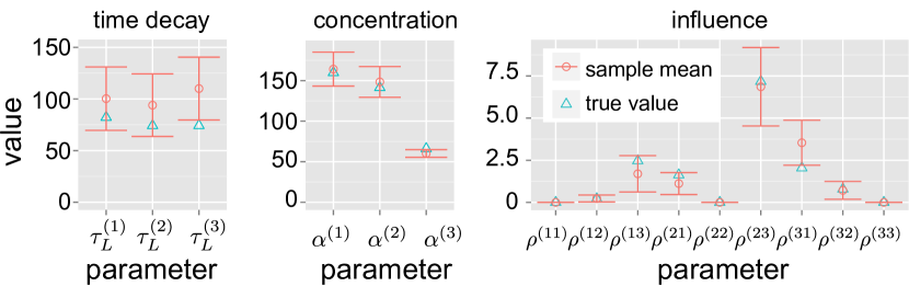
Figure 1: Parameter Recovery Results.

In this section, we present the results of a parameter recovery experiment, conducted in order to validate our inference algorithm. We used the generative process described in section 3 to generate 300 utterances made by $P=3$ people. In total, these utterances contain 15,070 tokens spanning $V=20$ types. We drew the length of each utterance, i.e., $L^{(p)}_{n}$, from a Poisson distribution with a mean of 50. We generated the start times and durations by assuming a round-robin approach to turn-taking and setting the duration of each utterance to a value proportional to its length in tokens. Figure 1 shows the true and inferred parameter values, depicted using blue triangles and red circles, respectively. The inferred parameter values were obtained by averaging 3,000 samples from the posterior distribution. The error bars indicate one standard deviation. Our proposed inference algorithm does well at accurately recovering the true parameter values.

5.2 Probability of Held-Out Data

The predictive probability of held-out data, sometimes expressed as perplexity, is a standard metric for evaluating statistical language models—the higher the probability, the better the model. We compared predictive probabilities obtained using the Bayesian Echo Chamber and several real-world data sets to those obtained using two comparable language models.

To compute the predictive probability of held-out data, we divided each data set into a training set $\{\mathcal{W}_{\textrm{train}},\mathcal{T}_{\textrm{train}},\mathcal{D}_{\textrm{train}}\}$ and a held-out or test set $\{\mathcal{W}_{\textrm{test}},\mathcal{T}_{\textrm{test}},\mathcal{D}_{\textrm{test}}\}$. We formed each training set by selecting those utterances that occurred before some time $t*$ where $t*$ was chosen to yield either a 90%–10% or 80%–20% training–testing split, i.e., $\mathcal{W}_{\textrm{train}}=\{\bm{w}_{n}^{(p)}:{t^{\prime}}_{n}^{(p)}\leq t*\}_{p=1}^{P}$ and $\mathcal{W}_{\textrm{test}}=\{\bm{w}_{m}^{(p)}:{t}_{m}^{(p)}>t*\}_{p=1}^{P}$. The predictive probability of held-out data is then $P(\mathcal{W}_{\textrm{test}}\,|\,\mathcal{T}_{\textrm{test}},\mathcal{D}_{\textrm{test}},\mathcal{W}_{\textrm{train}},\mathcal{T}_{\textrm{train}},\mathcal{D}_{\textrm{train}})$. Although this probability is analytically intractable, its logarithm can be approximated via the lower bound $\frac{1}{S}\sum_{s=1}^{S}\log{P(\mathcal{W}_{\textrm{test}}\,|\,\mathcal{T}_{\textrm{test}},\mathcal{D}_{\textrm{test}},\Theta^{(s)})}$ where $\Theta^{(s)}$ denotes a set of sampled parameter values drawn from the posterior distribution $P(\Theta\,|\,\mathcal{W}_{\textrm{train}},\mathcal{T}_{\textrm{train}},\mathcal{D}_{\textrm{train}})$.

Approximate log probabilities obtained using the Bayesian Echo Chamber (with $S=3000$ samples after 1000 burn-in sampling iterations), a unigram language model, and Blei and Lafferty’s dynamic topic model [2006] are provided in table 1. Log probabilities for additional data sets are provided in the supplementary material. The unigram language model is equivalent to setting all influence parameters in our model to zero. In all experiments involving the dynamic topic model, each data set was sliced into $K=10$ or $K=5$ equally-sized time slices (depending on the training–testing split), with the last slice taken to be the test set and utterances treated as documents. Each log probability reported for the dynamic topic model is the highest value obtained using either 5, 10, or 20 topics. Since inference for the dynamic topic model was performed using a variational inference algorithm, its log probabilities are also lower bounds and standard deviations are not available. For all data sets, the Bayesian Echo Chamber out-performed both the unigram language model and the dynamic topic model.

Table 1: Predictive Log Probabilities of Held-Out Data.

	10% Test Set					20% Test Set
Data Set	Our Model		Unigram		DTM	Our Model		Unigram		DTM
Synthetic	-4292.97$\pm$	0.02	-4297.92$\pm$	0.04	-4364.81	-8702.92$\pm$	0.04	-8717.77$\pm$	0.08	-8948.07
DC v. Heller	-7383.45$\pm$	0.12	-7794.25$\pm$	0.21	-7533.58	-12404.21$\pm$	0.15	-13126.73$\pm$	0.26	-12744.73
L&G v. Texas	-6663.33$\pm$	0.12	-6937.66$\pm$	0.18	-6759.06	-10248.80$\pm$	0.21	-10791.25$\pm$	0.23	-10459.87
Citizens United v. FEC	-5770.12$\pm$	0.14	-6120.67$\pm$	0.18	-5851.224	-16370.7$\pm$	0.95	-17157.21$\pm$	0.40	-16400.46
“12 Angry Men”	-4667.47$\pm$	0.24	-4920.21$\pm$	0.14	-4691.11	-8722.97$\pm$	0.27	-9222.99$\pm$	0.25	-8787.35

5.3 Influence Recovery

In this section, we demonstrate that the Bayesian Echo Chamber can recover known influence patterns in Supreme Court arguments and in the movie “12 Angry Men.” We also use these data sources to to compare influence networks inferred by our model to those inferred by the model described in section 2. All reported influence parameters were obtained by averaging 3,000 posterior samples; posterior standard deviations are provided in the supplementary material.

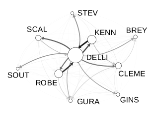
(a)

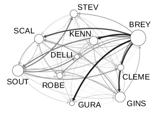
(b)

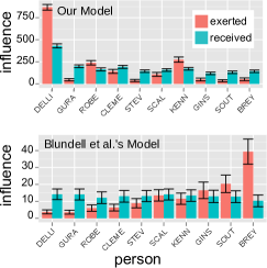
(c)

Figure 2: Influence Networks (Posterior Mean) Inferred from the DC v. Heller Case. (a) Network Inferred Using Our Model and (b) Inferred Using Blundell et al.’s Model. (c) Total Influence Exerted/Received by Each Person.

5.3.1 US Supreme Court

As described previously, Supreme Court arguments are extremely formulaic: The attorneys representing the petitioner present their argument first, speaking for a total of 30 minutes before the respondent’s attorneys are allowed to present their argument. Justices routinely interrupt these presentations. We therefore anticipate that influence networks inferred from linguistic accommodation patterns will reveal significant influence exerted by the petitioner’s attorneys, simply because they speak first, establishing the language used in the rest of the discussion. We also anticipate that influence networks inferred from turn-taking behavior will reveal significant influence exerted by the justices over the attorneys. This is because the justices interrogate the attorneys’ during their presentations.

As an illustrative example, we present results obtained from the District of Columbia v. Heller case in figure 2. (The other two cases, Lawrence and Garner v. Texas and Citizens United v. Federal Election Commission exhibited remarkably similar influence networks.) The influence network inferred using the Bayesian Echo chamber is shown in 2(a), while the network inferred using Blundell et al.’s model is shown in 2(b). To illustrate posterior uncertainty, networks drawn with different posterior quantiles are provided in the supplementary material. The total influence exerted and received by each participant are shown for each model in figure 2(c). The error bars represent the posterior standard deviation. The justices present for this case were Alito, Breyer, Ginsburg, Kennedy, Roberts, Scalia, Stevens, Souter, and Thomas, while the attorneys were Dellinger (representing the petitioner), Gura (representing the respondent), and Clement (as amicae curae, supporting the petitioner). Ultimately, Alito, Kennedy, Roberts, Scalia, and Thomas (the majority) sided with the respondent, while Breyer, Ginsburg, and Stevens (the minority) sided with the petitioner. Neither Alito or Thomas spoke ten or more utterances, so they were not included in our analyses.

The influence network inferred using our model is very sparse. As expected, Dellinger (who represented the petitioner and presented his argument first) is shown as exerting the most influence. The justices with the most influence are Kennedy and Roberts, both of whom ultimately supported the respondent and thus interrogated Dellinger much more the other justices.

The most striking pattern in the influence network inferred using Blundell et al.’s model is that the three attorneys received much more influence from the justices than vice versa. This pattern could be seen as reflecting the status difference between justices and attorneys or as reflecting the formulaic structure of the Supreme Court: attorneys present arguments, while justices interrupt to make comments or ask questions.

5.3.2 “12 Angry Men”

Unlike Supreme Court arguments, the dialog in “12 Angry Men” is informal and intended to seem natural. Since the focus of the movie is discussion-based consensus building in a group setting, we therefore anticipate that the narrative of the movie will be reflected in influence networks inferred from linguistic accommodation patterns and from turn-taking behavior.

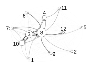
(a)

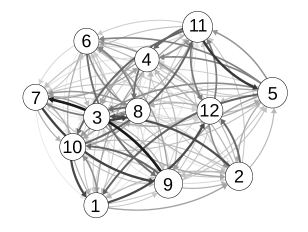
(b)

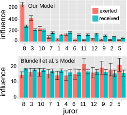
(c)

Figure 3: Influence Networks (Posterior Mean) Inferred from “12 Angry Men.” (a) Network Inferred Using Our Model and (b) Inferred Using Blundell et al.’s Model. (c) Total Influence Exerted/Received by Each Person.

The influence network inferred using our model is shown in figure 3(a), while the total influence exerted and received by each juror are shown in the top of figure  3(c). The most significant pattern is that three individuals exert more influence over others than others do over them: Juror 8, Juror 3, and, to a lesser extent, Juror 10. Juror 8 is the protagonist of the movie, and initially casts the only “not guilty” vote. The other jurors ultimately change their votes to match his. Juror 3, the antagonist, is the last to change his vote. It therefore unsurprising that Juror 8, the first to vote “not guilty”, should dominate the discussion content. Similarly, Juror 3, the last to change his “guilty” vote, is most invested in discussing defendant’s supposed guilt. Juror 10 is one of the last three jurors, along with Jurors 3 and 4, to change his vote. However, unlike Juror 4 (who stands out marginally in figure 3(a) and, according to figure 3(c), has less influence over others than others do over him), Juror 10 is argumentative as he changes his mind. Overall, the consistency of the inferred influence network with the narrative of the movie confirms that the Bayesian Echo Chamber can indeed uncover substantive influence relationships.

The influence network inferred using Blundell et al.’s model and the total influence exerted and received by each juror are shown in figure 3(b) and the bottom of 3(c), respectively. The four jurors who exert more influence over others than others do over them (Juror 2, Juror 5, Juror 9, and Juror 11) are the first four jurors to change their votes. Jurors 5 and 11, who exert the most influence, are verbose, while Jurors 2 and 9 are comparatively taciturn. Jurors 8 exerts little influence because he must respond to questions and defend his position as he tries to persuade the others to agree with him, much like the attorneys in the Supreme Court.

5.4 Exploratory Analysis of FOMC Meetings

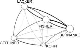
(a)

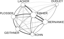
(b)

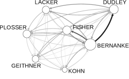
(c)

Figure 4: Influence Networks (Posterior Mean) Inferred from FOMC Meetings Using Our Model. (a) March 27, 2006–June 28, 2006. (b) August 8, 2006–August 7, 2007. (c) August 10, 2007–December 15, 2008.

Finally, we performed an exploratory analysis of the relationships inferred from transcripts of 32 Federal Open Market Committee meetings surrounding the 2007–2008 financial crisis, ranging from March 27, 2006 to December 15, 2008, inclusive. Since utterance durations are not available for these transcripts (also preventing the use of Blundell et al.’s model), we set the duration of each utterance to a value proportional to its length in tokens. We divided the meetings into three subsets: March 27, 2006 through June 28, 2006; August 8, 2006 through August 7, 2007; and August 10, 2007 through December 15, 2008. The first subset corresponds to meetings with a resultant policy of tightening; the second to meetings with a neutral outcome; and the third to meetings that resulted in easing. These meetings were all chaired by Bernanke.

Figure 4 depicts the influence network for each subset (aggregated by averaging over the meetings in that subset) inferred using our model. In the first network, corresponding to pre-crash meetings from March 27, 2006 through June 28, 2006, Bernanke, Fisher, and Lacker play the biggest roles with Bernanke, the chair, exerting the most influence over others. Given his role as chair, Bernanke’s involvement is arguably unsurprising, but Fisher and Lacker’s roles are notable. Unlike Bernanke, Fisher and Lacker are both “hawks” and thus generally in favor of tightening monetary policy; the meetings in this subset all resulted in an outcome of tightening. In the second network, corresponding to pre-crash meetings from August 8, 2006 through August 7, 2007, Bernanke, Fisher, and Lacker all continue to play significant roles, but the network is much less sparse, with both hawks and “doves” (those generally in favor of easing monetary policy) exerting influence over others. In contrast to the meetings in the previous subset, these meetings resulted in neutrality—i.e., neither tightening or easing. Finally, in the third network, corresponding to post-crash meetings from August 10, 2007 through December 15, 2008, there are fewer strong influence relationships. Bernanke (the chair and a dove) still plays a major role, while Fisher and Lacker’s roles are significantly diminished. Instead, Dudley, also a dove and a close ally of Bernanke, plays a much greater role, especially in his relationship with Bernanke. These meetings all resulted in monetary policy easing, a strategy generally favored by doves and opposed by hawks.

There has been little work in political science, economics, or computer science on analyzing these meeting transcripts. As a result, the inferred networks not only showcase our model’s ability to discover latent influence relationships from linguistic accommodation, but also constitute a research contribution of substantive interest to political scientists, economists, and other social scientists studying the financial crisis.

5.5 Model Combination

Since influence can be inferred from both turn-taking behavior and linguistic accommodation, we explored the possibility of combining the Bayesian Echo Chamber and Blundell et al.’s model to form a “supermodel” with a single set of shared influence parameters. The simplest way to share these parameters is to tie them together as $\rho^{(qp)}=r\nu^{(qp)}$, where $r$ is a scaling factor and $\rho^{(qp)}$ and $\nu^{(qp)}$ correspond to the influence from person $q$ to person $p$ in our model and Blundell et al.’s model, respectively. Tying the influence parameters in this way provides the model with the capacity to capture a global notion of influence that is based upon both turn-taking and linguistic accommodation.

This tied model, whose likelihood is the product of the Bayesian Echo Chamber’s likelihood and that of Blundell et al.’s model but with shared influence parameters, assigned lower probabilities to held-out data than the fully factorized model (i.e., separate influence parameters). Log probabilities, obtained using a 90%–10% training–testing split and a vocabulary of $V=300$ word types in order to reduce computation time, are provided in the supplementary material.

Interestingly, the networks inferred by the model with tied parameters are extremely similar to those inferred using the Bayesian Echo Chamber. These results suggest that linguistic accommodation reflects a more informative notion of influence that that evidenced via turn-taking. We expect that investigating other ways of combining turn-taking-based models with ours will be a promising direction for future exploration.

6 DISCUSSION

The Bayesian Echo Chamber is a new generative model for discovering latent influence networks via linguistic accommodation patterns. We demonstrated that our model can recover known influence patterns in synthetic data, arguments heard by the US Supreme Court, and in the movie “12 Angry Men.” We compared influence networks inferred using our model to those inferred using a variant of Blundell et al.’s turn-taking-based model and showed that by modeling linguistic accommodation patterns, our model infers different, and often more meaningful, influence networks. Finally, we showcased our model’s potential as an exploratory analysis tool for social scientists by inferring latent influence relationships between members of the Federal Reserve’s Federal Open Market Committee.

Promising avenues for future work include (1) modeling linguistic accommodation separately for function and content words and (2) explicitly modeling the dynamic evolution of influence networks over time.

Acknowledgements

Thanks to Juston Moore and Aaron Schein for their work on early stages of this project, and to Aaron for the “Bayesian Echo Chamber” model name. This work was supported in part by the Center for Intelligent Information Retrieval, in part by NSF grant #IIS-1320219, and in part by NSF grant #SBE-0965436. Any opinions, findings and conclusions or recommendations expressed in this material are the authors’ and do not necessarily reflect those of the sponsor.

 

Supplementary Material for “The Bayesian Echo Chamber”

 

Fangjian Guo                        Charles Blundell                        Hanna Wallach                        Katherine Heller

Duke University Durham, NC, USA guo@cs.duke.edu                        Gatsby Unit, UCL London, UK c.blundell@gatsby.ucl.ac.uk                        Microsoft Research New York, NY, USA   wallach@microsoft.com                        Duke University Durham, NC, USA kheller@stat.duke.edu

1 INFLUENCE VIA TURN-TAKING

In this section, we provide appropriate priors and details of an inference algorithm for the variant of Blundell et al.’s model [BluHelBec2012a] described in section 2 of the paper. For real-world group discussions, the utterance start times $\mathcal{T}=\{\mathcal{T}^{(p)}\}_{p=1}^{P}$ and durations $\mathcal{D}=\{\{\Delta t_{n}^{(p)}\}_{n=1}^{N^{(p)}(T)}\}_{p=1}^{P}$ are observed, while parameters $\Theta=\{\lambda_{0}^{(p)},\{\nu^{(qp)}\}_{q\neq p},\tau_{T}^{(p)}\}_{p=1}^{P}$ are unobserved; however, information about the values of these parameters can be quantified via their posterior distribution given $\mathcal{T}$ and $\mathcal{D}$, obtained via Bayes’ theorem, i.e.,

$$P(\Theta\,|\,\mathcal{T},\mathcal{D})\propto P(\mathcal{T}\,|\,\Theta,\mathcal{D})\,P(\Theta).$$ (5)

The likelihood term has the form

$$P(\mathcal{T}\,|\,\Theta,\mathcal{D})=$$

$$\quad\prod_{p=1}^{P}\left(\exp{\left(-\Lambda^{(p)}(T)\right)}\prod_{n=1}^{N^{(p)}(T)}\lambda^{(p)}(t_{n}^{(p)})\right),$$ (6)

where $\Lambda^{(p)}(T)=\int_{0}^{T}\lambda^{(p)}(t)\,\textrm{d}t$ is the expected total number of utterances made over the entire observation interval from $0$ to $T$ [daley88introduction].

Like Blundell et al., we place an improper prior over $\lambda_{0}^{(p)}>0$. We also use priors to ensure that the multivariate Hawkes process is stationary. Specifically, we employ the stationarity condition of bremaud96stability. If $\bm{M}$ is a $P\times P$ matrix given by

$$M^{(qp)}=\int_{u}^{\infty}\left|\,g^{(qp)}(t,u)\right|\,\textrm{d}t=\nu^{(qp)}\tau^{(p)}_{T},$$ (7)

then this condition requires the spectral radius of $\bm{M}$ to be strictly less than one. This condition is not straightforward to enforce with tractable constraints; however, since the spectral radius of $\bm{M}$ is upper-bounded by any matrix norm, the condition may be enforced by requiring that $\|\bm{M}\|<1$ for any norm $\|\cdot\|$. We use the maximum absolute column sum norm:

$$\|\bm{M}\|_{1\rightarrow 1} =\max_{\|x\|_{1}=1}\|\bm{M}x\|_{1}$$ (8)

$$=\max_{p=1,\cdots,P}\tau_{T}^{(p)}\sum_{q\neq p}\nu^{(qp)}.$$ (9)

Rewriting this expression implies an improper joint prior over $\{\tau_{T}^{(p)}\}_{p=1}^{P}$ and $\{\{\nu^{(qp)}\}_{q\neq p}\}_{p=1}^{P}$ in which

$$0<\tau_{T}^{(p)}<\frac{1}{\sum_{q\neq p}\nu^{(qp)}}\textrm{ and }$$ (10)

$$\quad 0<\nu^{(qp)}<\frac{1}{\tau_{T}^{(p)}-\sum_{r\neq q,r\neq p}}\nu^{(rp)}.$$ (11)

Although the resultant posterior distribution $P(\Theta\,|\,\mathcal{T},\mathcal{D})$ is analytically intractable, posterior samples can be drawn using either the conditional intensity function approach or the cluster process approach described by rasmussen2013bayesian. Like Blundell et al., we take the former approach and use a slice-within-Gibbs algorithm [Neal2003] that sequentially samples each parameter from its conditional posterior.

This slice-within-Gibbs algorithm requires frequent evaluation of the likelihood in equation 6; however, the computational cost can be reduced by noting that the product over rate functions can be efficiently computed using the following recurrence relation:

$$\lambda^{(p)}(t_{n}^{(p)})=$$

$$\quad\lambda_{0}^{(p)}+\left(\lambda^{(p)}(t_{n-1}^{(p)})-\lambda_{0}^{(p)}\right)\exp{\left(-\frac{t_{n}^{(p)}-t_{n-1}^{(p)}}{\tau_{T}^{(p)}}\right)}+{}$$

$$\quad\sum_{q\neq p}\sum_{m:t_{n-1}^{(p)}\leq{t^{\prime}}_{m}^{(q)}<t_{n}^{(p)}}\nu^{(qp)}\exp{\left(-\frac{t_{n}^{(p)}-{t^{\prime}}_{m}^{(q)}}{\tau_{T}^{(p)}}\right)}$$

for $n=2,3,\ldots,N^{(p)}(T)$. The initial term is

$$\lambda^{(p)}(t_{1}^{(p)})=$$

$$\quad\lambda_{0}^{(p)}+\sum_{q\neq p}\sum_{m:{t^{\prime}}_{m}^{(q)}<t_{1}^{(p)}}\nu^{(qp)}\exp{\left(-\frac{t^{(p)}_{1}-{t^{\prime}}_{m}^{(q)}}{\tau_{T}^{(p)}}\right)}.$$

2 INFLUENCE VIA LINGUISTIC ACCOMMODATION

In this section, we provide a directed graphical model, appropriate priors, and details of an inference algorithm for our model, the Bayesian Echo Chamber.

The likelihood term implied by our model is

$$P(\mathcal{W}\,|\,\Theta,\mathcal{T},\mathcal{D})=$$

$$\quad\prod_{p=1}^{P}\prod_{n=1}^{N^{(p)}(T)}P(\bm{w}_{n}^{(p)}\,|\,\{\{\bm{w}_{m}^{(q)}\}_{m:{t^{\prime}}_{m}^{(q)}<t^{(p)}_{n}}\}_{q\neq p},\Theta).$$

A directed graphical model depicting the structure of $P(\bm{w}_{n}^{(p)}\,|\,\{\{\bm{w}_{m}^{(q)}\}_{m:{t^{\prime}}_{m}^{(q)}<t^{(p)}_{n}}\}_{q\neq p},\Theta)$ is in figure 5.

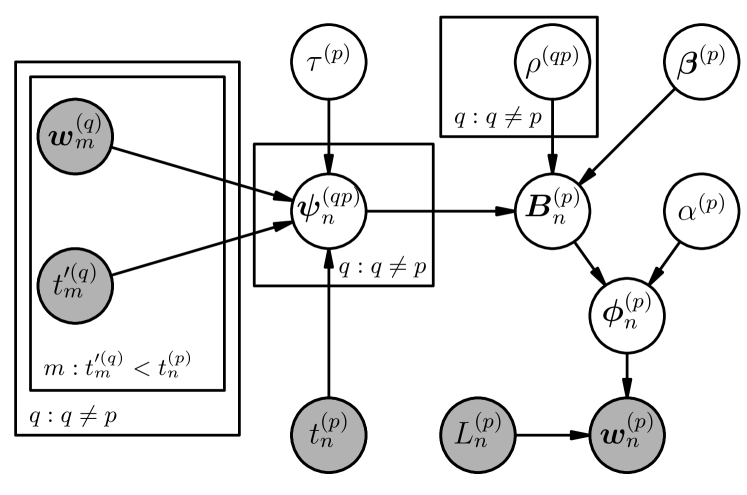
Figure 5: Directed Graphical Model Depicting the Structure of $P(\bm{w}_{n}^{(p)}\,|\,\{\{\bm{w}_{m}^{(q)}\}_{m:{t^{\prime}}_{m}^{(q)}<t^{(p)}_{n}}\}_{q\neq p},\Theta)$.

We place a gamma prior over $\rho^{(qp)}$, with a shape parameter chosen to encourage shrinkage towards zero. Due to the additive nature of $\bm{B}_{n}^{(p)}$, the value of $\beta_{v}^{(p)}$ should be comparable in magnitude to $\sum_{q\neq p}\rho^{(qp)}\psi_{v,n}^{(qp)}$. We therefore place a gamma prior over each $\beta_{v}^{(p)}$, with shape and scale parameters chosen to yield this property for real-world data sets. We also place broad gamma priors over $\alpha^{(p)}$ and $\tau_{L}^{(p)}$. In practice, inference is insensitive to the specific values of the shape and scale parameters of these priors, provided they are broad. For our experiments, we used $\alpha^{(p)}\sim\textrm{Gamma}\,(10,10)$, $\beta_{v}^{(p)}\sim\textrm{Gamma}\,(10,20)$, $\rho^{(qp)}\sim\textrm{Gamma}\,(1,2)$, and $\tau^{(p)}\sim\textrm{Gamma}\,(10,10)$.

Although the resultant posterior distribution $P(\Theta\,|\,\mathcal{W},\mathcal{T},\mathcal{D})$ is intractable, posterior samples of $\{\alpha^{(p)},\bm{\beta}^{(p)},\{\rho^{(qp)}\}_{q\neq p},\tau_{L}^{(p)}\}_{p=1}^{P}$ can be drawn using a collapsed slice-with-Gibbs algorithm that sequentially samples each parameter from its conditional posterior. Pseudocode for this approach is given in algorithm 1. Each parameter is sampled in a univariate fashion, except for $\bm{\beta}^{(p)}$, which is drawn using multivariate slice sampling with the hyperractangle method [Neal2003]. To improve mixing, we drew ten samples of $\bm{\beta}^{(p)}$ during each Gibbs sweep. When implemented in Python, we were able to draw 4,000 posterior samples (including 1,000 burn-in samples) of $\{\alpha^{(p)},\bm{\beta}^{(p)},\{\rho^{(qp)}\}_{q\neq p},\tau_{L}^{(p)}\}_{p=1}^{P}$ in at most a couple of hours for all data sets used in our experiments.

Algorithm 1 Inference Algorithm

for $i=1,2,\cdots,I$ do

     for $p=1,2,\cdots,P$ do

         Slice sample $\alpha^{(p)}$

         Slice sample $\tau^{(p)}_{L}$

         for $q\neq p$ do

              Slice sample $\rho^{(qp)}$

         end for

         for $j=1,2,\cdots,10$ do

              Slice sample $\bm{\beta}^{(p)}$ (multivariate)

         end for

     end for

end for

3 EXPERIMENTS

The salient characteristics of all data sets used in our experiments are provided in table 2. For each data set obtained from TalkBank [macwhinney2007talkbank], the “TalkBank” column contains the data set identifier within the “Meetings” section of the TalkBank database. The “No. Tokens” column indicates the total number of tokens in each data set after restricting the vocabulary to the $V=600$ most frequent stemmed types. The “Tokens Removed” column contains the percentage of tokens that were discarded via this step.

Table 2: Salient Characteristics of Data Sets.

Data Set	TalkBank	No. People	No. Utterances	No. Tokens	Tokens Removed
Synthetic	–	3	300	15,070	0.00%
University Lecture	SB/12	5	138	3,482	4.42%
Birthday Party	SB/49	8	454	4,229	5.88%
DC v. Heller	SCOTUS/07-290	10	365	15,104	7.21%
L&G v. Texas	SCOTUS/02-102	6	200	8,573	5.47%
Citizens United v. FEC	SCOTUS/08-205b	10	345	12,700	7.41%
12 Angry Men	–	12	312	6,350	5.25%
January 29, 2008 FOMC Meeting	–	4	101	13,505	13.74%

Table 3 contains predictive log probabilities for several additional data sets. The “Family Discussion” and “University Lecture” data sets are conversation transcripts from the Santa Barbara Corpus of Spoken American English [macwhinney2007talkbank]. These data sets capture the back-and-forth of real-world conversations. The “January 29, 2008 FOMC Meeting” data set is one of the FOMC meeting transcripts used our exploratory analysis. The salient characteristics of these data sets are given in table 2. For all but one of these additional data sets, the Bayesian Echo Chamber out-performed a unigram language model and Blei and Lafferty’s dynamic topic model [blei06dynamic] by predicting higher probabilities of held-out data for both a 90%–10% and an 80%–20% training–testing split.

Table 3: Additional Predictive Log Probabilities of Held-Out Data.

	10% Test Set					20% Test Set
Data Set	Our Model		Unigram		DTM	Our Model		Unigram		DTM
University Lecture	-528.23$\pm$	0.06	-541.23$\pm$	0.05	-520.74	-1972.67$\pm$	0.13	-2009.62$\pm$	0.12	-2110.66
Birthday Party	-1883.45$\pm$	0.11	-1961.4$\pm$	0.11	-1900.68	-4384.42$\pm$	0.16	-4625.57$\pm$	0.20	-4498.467
January 29, 2008 FOMC Meeting	-3187.73$\pm$	0.04	-3338.59$\pm$	0.10	-3211.09	-17342.43$\pm$	0.21	-17779.01$\pm$	0.24	-17726.64

Posterior means and standard deviations of the influence parameters $\{\{\rho^{(qp)}\}_{q\neq p}\}_{p=1}^{P}$ inferred from the DC v. Heller Supreme Court case using our model are given in tables 4 and 5, respectively. These values were obtained using 3,000 samples from the posterior distribution. To further illustrate posterior uncertainty, influence networks drawn using 25%, 50% (i.e., median), and 75% posterior quantiles are shown in figure 6. These networks look very similar to each other.

Table 4: Posterior Means of $\{\{\rho^{(qp)}\}_{q\neq p}\}_{p=1}^{P}$ Inferred from the DC v. Heller Case.

	To
From	DELLI	GURA	ROBE	CLEME	STEV	SCAL	KENN	GINS	SOUT	BREY
DELLI	–	65.85	109.92	109.36	86.78	125.29	143.29	71.21	82.77	72.98
GURA	10.18	–	4.79	2.43	7.75	3.27	2.62	3.17	6.84	5.08
ROBE	161.29	37.99	–	6.44	3.76	5.12	4.77	7.62	3.99	7.67
CLEME	5.12	37.41	11.02	–	16.53	4.84	6.03	15.77	12.53	32.13
STEV	3.93	9.27	3.89	4.37	–	3.10	2.70	2.91	4.42	3.12
SCAL	50.53	15.45	7.77	5.62	4.64	–	3.41	6.04	7.17	6.83
KENN	180.91	2.90	5.86	50.67	13.75	4.93	–	4.50	5.53	5.63
GINS	6.98	9.91	11.29	4.55	3.22	4.08	2.69	–	2.95	3.68
SOUT	3.34	4.34	3.86	5.90	3.55	3.54	2.59	3.22	–	4.50
BREY	8.24	16.48	5.18	2.45	3.71	3.22	2.99	4.31	5.26	–

Table 5: Posterior Standard Deviations of $\{\{\rho^{(qp)}\}_{q\neq p}\}_{p=1}^{P}$ Inferred from the DC v. Heller Case.

	To
From	DELLI	GURA	ROBE	CLEME	STEV	SCAL	KENN	GINS	SOUT	BREY
DELLI	–	7.36	11.08	8.99	10.30	12.25	12.73	10.12	10.94	9.22
GURA	6.12	–	3.88	2.34	5.90	3.07	2.51	3.12	5.20	4.39
ROBE	14.60	12.93	–	5.76	3.48	4.92	4.75	6.68	3.91	7.48
CLEME	4.69	6.32	7.11	–	9.73	4.45	5.15	9.35	8.49	8.81
STEV	3.65	7.56	3.68	4.16	–	3.12	2.73	2.99	4.40	3.08
SCAL	14.02	9.42	6.84	5.02	4.43	–	3.33	5.67	6.46	6.28
KENN	14.84	2.70	5.46	17.43	10.61	4.68	–	4.14	5.13	5.64
GINS	6.32	8.14	9.74	4.24	3.09	4.09	2.58	–	2.79	3.56
SOUT	3.52	4.11	3.75	5.85	3.72	3.25	2.47	3.16	–	4.86
BREY	7.19	8.40	4.89	2.43	3.58	3.05	2.95	3.91	4.53	–

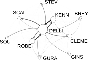
(a)

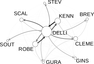
(b)

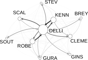
(c)

Figure 6: Influence Networks for the DC v. Heller Case Drawn Using (a) 25%, (b) 50%, and (c) 75% Quantiles.

Posterior means and standard deviations of the influence parameters $\{\{\rho^{(qp)}\}_{q\neq p}\}_{p=1}^{P}$ inferred from “12 Angry Men” using our model are provided in tables 6 and 7, respectively. These values were obtained using 3,000 samples from the posterior distribution. To further illustrate posterior uncertainty, influence networks drawn using 25%, 50%, and 75% posterior quantiles are provided in figure 7. As with the DC v. Heller case, these networks look very similar to one another.

Table 6: Posterior Means of $\{\{\rho^{(qp)}\}_{q\neq p}\}_{p=1}^{P}$ Inferred from “12 Angry Men.”

	To
From	Juror 8	Juror 3	Juror 10	Juror 7	Juror 1	Juror 4	Juror 6	Juror 11	Juror 12	Juror 9	Juror 2	Juror 5
Juror 8	–	82.09	61.82	61.08	39.80	80.38	75.30	48.96	80.12	72.86	43.58	33.98
Juror 3	134.35	–	112.40	47.76	27.56	59.83	10.62	6.46	16.85	5.28	5.51	6.84
Juror 10	53.38	88.01	–	30.65	24.54	4.71	12.72	3.41	9.48	4.08	4.25	5.50
Juror 7	19.56	11.53	13.97	–	8.24	3.69	5.19	3.35	4.46	4.25	4.86	4.08
Foreman	5.12	5.51	3.30	2.99	–	3.02	3.74	2.66	4.82	2.57	3.11	3.18
Juror 4	43.05	11.73	2.88	2.88	3.44	–	2.47	46.62	4.08	6.47	4.55	3.46
Juror 6	5.79	3.23	3.03	3.16	2.76	2.56	–	2.82	3.14	3.11	3.30	3.23
Juror 11	3.39	2.76	2.63	2.17	2.28	2.80	2.32	–	2.61	2.50	2.40	2.44
Juror 12	9.61	3.49	3.00	3.47	2.84	2.91	4.44	3.59	–	2.64	3.62	2.76
Juror 9	4.28	3.44	2.56	2.95	2.68	2.73	2.96	4.44	3.05	–	2.67	2.82
Juror 2	2.85	2.99	2.84	2.67	3.34	2.41	3.34	2.16	3.14	2.49	–	3.05
Juror 5	2.88	2.49	2.59	2.38	2.54	2.23	2.47	2.77	2.53	2.73	2.35	–

Table 7: Posterior Standard Deviations of $\{\{\rho^{(qp)}\}_{q\neq p}\}_{p=1}^{P}$ Inferred from “12 Angry Men.”

	To
From	Juror 8	Juror 3	Juror 10	Juror 7	Juror 1	Juror 4	Juror 6	Juror 11	Juror 12	Juror 9	Juror 2	Juror 5
Juror 8	–	13.10	14.50	14.09	14.12	14.54	13.52	12.53	13.51	11.50	12.35	11.31
Juror 3	15.21	–	18.19	17.49	16.01	16.63	8.71	5.76	12.62	4.86	5.00	6.17
Juror 10	14.47	16.84	–	17.76	14.06	4.36	10.20	3.33	8.20	3.82	4.22	5.15
Juror 7	12.34	10.15	10.36	–	7.30	3.44	4.91	3.09	4.66	4.08	4.57	3.80
Foreman	4.58	5.18	3.42	3.12	–	3.10	3.80	2.63	4.66	2.57	3.16	3.06
Juror 4	12.45	9.17	2.84	2.81	3.32	–	2.44	15.45	4.04	6.41	4.27	3.38
Juror 6	5.51	3.42	3.04	3.14	2.66	2.44	–	2.72	3.06	3.06	3.43	3.30
Juror 11	3.46	2.75	2.55	2.26	2.26	2.77	2.28	–	2.60	2.47	2.33	2.41
Juror 12	8.14	3.38	3.00	3.44	2.76	2.87	4.24	3.51	–	2.63	3.46	2.63
Juror 9	4.35	3.39	2.51	2.97	2.64	2.70	2.90	4.59	3.00	–	2.58	2.76
Juror 2	2.79	2.90	2.68	2.64	3.42	2.23	3.41	2.20	3.07	2.49	–	3.21
Juror 5	2.83	2.53	2.68	2.49	2.46	2.28	2.55	2.76	2.63	2.80	2.35	–

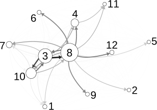
(a)

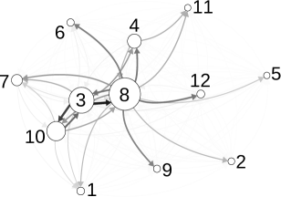
(b)

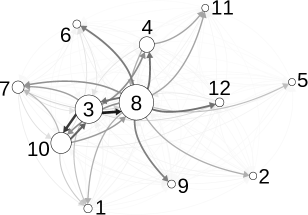
(c)

Figure 7: Influence Networks for “12 Angry Men” Drawn Using (a) 25%, (b) 50%, and (c) 75% Quantiles.

Log probabilities, obtained using a 90%–10% training–testing split and a vocabulary of $V=300$ types, are provided for the tied and untied combined models in table 8. The tied model, whose likelihood is the product of the Bayesian Echo Chamber’s likelihood and that of Blundell et al.’s model but with shared influence parameters, assigned lower probabilities to held-out data than the fully factorized (i.e., untied) model.

Data Set	Tied		Untied
L&G v. Texas	-5507.11$\pm$	0.15	-5502.87$\pm$	0.15
DC v. Heller	-6321.30$\pm$	0.16	-6303.55$\pm$	0.15
Citizens United v. FEC	-4795.24$\pm$	0.18	-4777.96$\pm$	0.17
“12 Angry Men”	-4014.56$\pm$	0.24	-3987.20$\pm$	0.23

Table 8: Log Probabilities of Held-Out Data for the Combined Model with Tied and Untied Parameters.

Acknowledgements

Thanks to Juston Moore and Aaron Schein for their work on early stages of this project, and to Aaron for the “Bayesian Echo Chamber” model name. This work was supported in part by the Center for Intelligent Information Retrieval, in part by NSF grant #IIS-1320219, and in part by NSF grant #SBE-0965436. Any opinions, findings and conclusions or recommendations expressed in this material are the authors’ and do not necessarily reflect those of the sponsor.

References

- Backstrom et al., [2006] Backstrom, L., Huttenlocher, D., Kleinberg, J., and Lan, X. (2006). Group formation in large social networks: Membership, growth, and evolution. In Proceedings of the 12th ACM SIGKDD International Conference on Knowledge Discovery and Data Mining.
- Blei and Lafferty, [2006] Blei, D. M. and Lafferty, J. D. (2006). Dynamic topic models. In Proceedings of the 23rd International Conference on Machine Learning.
- Blundell et al., [2012] Blundell, C., Heller, K. A., and Beck, J. (2012). Modelling reciprocating relationships with Hawkes processes. In Advances In Neural Information Processing Systems.
- Bremaud and Massouli, [1996] Bremaud, P. and Massouli, L. (1996). Stability of nonlinear Hawkes processes. The Annals of Probability, pages 1563–1588.
- Daley and Vere-Jones, [1988] Daley, D. J. and Vere-Jones, D. (1988). An Introduction to the Theory of Point Processes. Springer.
- Danescu-Niculescu-Mizil et al., [2012] Danescu-Niculescu-Mizil, C., Lee, L., Pang, B., and Kleinberg, J. (2012). Echoes of power: Language effects and power differences in social interaction. In Proceedings of the 21st International Conference on World Wide Web, pages 699–708.
- de Solla Price, [1965] de Solla Price, D. J. (1965). Networks of scientific papers. Science, 149(3683):510–515.
- DuBois et al., [2013] DuBois, C., Butts, C., and Smyth, P. (2013). Stochastic blockmodeling of relational event dynamics. In Proceedings of the Sixteenth International Conference on Artificial Intelligence and Statistics, pages 238–246.
- Epskamp et al., [2012] Epskamp, S., Cramer, A. O., Waldorp, L. J., Schmittmann, V. D., and Borsboom, D. (2012). qgraph: Network visualizations of relationships in psychometric data. Journal of Statistical Software, 48(4):1–18.
- Fowler, [2006] Fowler, J. H. (2006). Legislative cosponsorship networks in the US House and Senate. Social Networks, 28:454–465.
- Gerrish and Blei, [2010] Gerrish, S. M. and Blei, D. M. (2010). A language-based approach to measuring scholarly impact. In Proceedings of the 26th International Conference on Machine Learning.
- Hawkes, [1971] Hawkes, A. G. (1971). Point spectra of some self-exciting and mutually exciting point processes. Journal of the Royal Statistical Society: Series B (Methodology), 58:83–90.
- Iwata et al., [2013] Iwata, T., Shah, A., and Ghahramani, Z. (2013). Discovering latent influence in online social activities via shared cascade Poisson processes. In Proceedings of the 19th ACM SIGKDD International Conference on Knowledge Discovery and Data Mining, pages 266–274.
- Linderman and Adams, [2014] Linderman, S. W. and Adams, R. P. (2014). Discovering latent network structure in point process data. International Conference on Machine Learning (ICML).
- MacWhinney, [2007] MacWhinney, B. (2007). The TalkBank project. Creating and Digitizing Language Corpora: Synchronic Databases.
- Neal, [2003] Neal, R. M. (2003). Slice sampling. Annals of Statistics, 31(3):705–767.
- Perry and Wolfe, [2013] Perry, P. O. and Wolfe, P. J. (2013). Point process modelling for directed interaction networks. Journal of the Royal Statistical Society: Series B (Methodology), 75(5):821–849.
- Rasmussen, [2013] Rasmussen, J. G. (2013). Bayesian inference for hawkes processes. Methodology and Computing in Applied Probability, 15(3):623–642.
- Simma and Jordan, [2010] Simma, A. and Jordan, M. I. (2010). Modeling events with cascades of Poisson processes. Proceedings of Uncertainty in Artificial Intelligence.
- West and Turner, [2010] West, R. and Turner, L. (2010). Introducting Communication Theory: Analysis and Applications. McGraw Hill.
- Zhou et al., [2013] Zhou, K., Zha, H., and Song, L. (2013). Learning triggering kernels for multi-dimensional Hawkes processes. In Proceedings of the 30th International Conference on Machine Learning, pages 1301–1309.

References

- Backstrom et al., [2006] Backstrom, L., Huttenlocher, D., Kleinberg, J., and Lan, X. (2006). Group formation in large social networks: Membership, growth, and evolution. In Proceedings of the 12th ACM SIGKDD International Conference on Knowledge Discovery and Data Mining.
- Blei and Lafferty, [2006] Blei, D. M. and Lafferty, J. D. (2006). Dynamic topic models. In Proceedings of the 23rd International Conference on Machine Learning.
- Blundell et al., [2012] Blundell, C., Heller, K. A., and Beck, J. (2012). Modelling reciprocating relationships with Hawkes processes. In Advances In Neural Information Processing Systems.
- Bremaud and Massouli, [1996] Bremaud, P. and Massouli, L. (1996). Stability of nonlinear Hawkes processes. The Annals of Probability, pages 1563–1588.
- Daley and Vere-Jones, [1988] Daley, D. J. and Vere-Jones, D. (1988). An Introduction to the Theory of Point Processes. Springer.
- Danescu-Niculescu-Mizil et al., [2012] Danescu-Niculescu-Mizil, C., Lee, L., Pang, B., and Kleinberg, J. (2012). Echoes of power: Language effects and power differences in social interaction. In Proceedings of the 21st International Conference on World Wide Web, pages 699–708.
- de Solla Price, [1965] de Solla Price, D. J. (1965). Networks of scientific papers. Science, 149(3683):510–515.
- DuBois et al., [2013] DuBois, C., Butts, C., and Smyth, P. (2013). Stochastic blockmodeling of relational event dynamics. In Proceedings of the Sixteenth International Conference on Artificial Intelligence and Statistics, pages 238–246.
- Epskamp et al., [2012] Epskamp, S., Cramer, A. O., Waldorp, L. J., Schmittmann, V. D., and Borsboom, D. (2012). qgraph: Network visualizations of relationships in psychometric data. Journal of Statistical Software, 48(4):1–18.
- Fowler, [2006] Fowler, J. H. (2006). Legislative cosponsorship networks in the US House and Senate. Social Networks, 28:454–465.
- Gerrish and Blei, [2010] Gerrish, S. M. and Blei, D. M. (2010). A language-based approach to measuring scholarly impact. In Proceedings of the 26th International Conference on Machine Learning.
- Hawkes, [1971] Hawkes, A. G. (1971). Point spectra of some self-exciting and mutually exciting point processes. Journal of the Royal Statistical Society: Series B (Methodology), 58:83–90.
- Iwata et al., [2013] Iwata, T., Shah, A., and Ghahramani, Z. (2013). Discovering latent influence in online social activities via shared cascade Poisson processes. In Proceedings of the 19th ACM SIGKDD International Conference on Knowledge Discovery and Data Mining, pages 266–274.
- Linderman and Adams, [2014] Linderman, S. W. and Adams, R. P. (2014). Discovering latent network structure in point process data. International Conference on Machine Learning (ICML).
- MacWhinney, [2007] MacWhinney, B. (2007). The TalkBank project. Creating and Digitizing Language Corpora: Synchronic Databases.
- Neal, [2003] Neal, R. M. (2003). Slice sampling. Annals of Statistics, 31(3):705–767.
- Perry and Wolfe, [2013] Perry, P. O. and Wolfe, P. J. (2013). Point process modelling for directed interaction networks. Journal of the Royal Statistical Society: Series B (Methodology), 75(5):821–849.
- Rasmussen, [2013] Rasmussen, J. G. (2013). Bayesian inference for hawkes processes. Methodology and Computing in Applied Probability, 15(3):623–642.
- Simma and Jordan, [2010] Simma, A. and Jordan, M. I. (2010). Modeling events with cascades of Poisson processes. Proceedings of Uncertainty in Artificial Intelligence.
- West and Turner, [2010] West, R. and Turner, L. (2010). Introducting Communication Theory: Analysis and Applications. McGraw Hill.
- Zhou et al., [2013] Zhou, K., Zha, H., and Song, L. (2013). Learning triggering kernels for multi-dimensional Hawkes processes. In Proceedings of the 30th International Conference on Machine Learning, pages 1301–1309.