Statistical distributions of pyrosequencing

Abstract

Pyrosequencing is emerging as one of the important next-generation sequencing technologies. We derive the statistical distributions of this technique in terms of nucleotide probabilities of the target sequences. We give exact distributions both for fixed number of flow cycles and for fixed sequence length. Explicit formulas are derived for the mean and variance of these distributions. In both cases, the distributions can be approximated accurately by normal distributions with the same mean and variance. The statistical distributions will be useful for instrument and software development for pyrosequencing platforms.

1 Introduction

The emerging new sequencing platforms, the so-called next-generation sequencing technology, have enabled researchers to generate more sequencing data than ever before with a dramatically reduced cost. The innovations have already transformed the way biology experiments are carried out. Unlike the traditional Sanger capillary electrophoresis method using dideoxynucleotide chain-termination, many of these new platforms explore the concept of sequencing by synthesis. Pyrosequencing technique is one of such approaches (Ronaghi et al., 1998). Compared with other next-generation sequencing techniques, currently the pyrosequencing technology has the advantage of longer sequence read length, which makes it possible for de novo sequencing of new genomes.

In this paper we derive the statistical distributions for the pyrosequencing technique. These distributions are useful for various stages in the use and development of the pyrosequencing technology, such as instrument development and testing, algorithm and software development, and the everyday machine performance monitoring and trouble-shooting.

The distribution of the number of flow cycles for sequences with fixed length and the distribution of sequence length at fixed number of flow cycles are obtained. In both cases the distributions can be approximated quite accurately by normal distributions with the same mean and variance as the exact distributions. We obtained the distributions by using the method of probability generating functions (GFs), which in turn were obtained by using the recurrence relations between the probabilities at different sequence lengths and flow cycles.

The paper is organized as follows. First in the remaining of this Introduction section we give a brief description of the pyrosequencing technique, which is useful for the subsequent theoretical developments. We also define the necessary notation here. The derivation of the main results, which are exact under the assumptions of the sequence model, will be presented in the Bivariate Generating Functions section. After that, we present the explicit formulas for the mean and variance of the distributions, for both fixed number of cycles and fixed sequences length. We show that the exact distributions can be approximated accurately by normal distributions with the same mean and variance calculated from these formulas. These explicit formulas would be most useful for the practitioners in the field. We also present the results for individual flows (the four different nucleotides) in this section.

1.1 Pyrosequencing technique

Pyrosequencing protocol is based on the detection of the pyrophosphate (PPi) that is released during DNA synthesis. In most of the current systems, several enzymes are involved in the chemical reactions. The protocol adds the four kinds of nucleotides (dATP, dCTP, dGTP, and dTTP) stepwise and iteratively, with one kind of nucleotide at a time. For each nucleotide flow, if the added nucleotide is complementary to the DNA template being sequenced, the added nucleotide is incorporated by polymerase. Inorganic PPi is released as a result of the polymerization reaction, which is converted to ATP by ATP sulfurylase. The ATP provides energy for luciferase to oxidize luciferin and to generate detectable light quantitatively. Because we know which nucleotide is added at each nucleotide flow, the DNA sequence of the template can be determined by the presence or absence of the emitted light and the intensity of the emitted light. The detected light is usually presented as a pyrogram, in which the x-axis is the pre-determined nucleotide flows and y-axis is the intensity of the emitted light at each nucleotide flow. Excess nucleotides are enzymatically degraded before the next nucleotide is added. Ideally the intensity of the light is proportional to the number of incorporated nucleotides. In reality this is not always the case due to the nonlinear light response following incorporation of more than a few identical nucleotides. This poses an inherent difficulty for the pyrosequencing protocol to determine the homopolymeric region accurately.

1.2 Notation and definitions

To avoid the unnecessary specification of the detailed names of the four kinds of nucleotides, in the following we will use $a$, $b$, $c$, and $d$ to represent any permutations of the usual nucleotides $A$, $C$, $G$, and $T$. Throughout the paper we assume that the nucleotides in the target sequence are independent of each other. The probabilities for the four nucleotides in the target sequence are denoted as $p_{a}$, $p_{b}$, $p_{c}$, and $p_{d}$. In Table 1 we define the nucleotide flow cycle number $f$ (the third row) to distinguish it from nucleotide flow number (the second row). A flow cycle is the “quad cycle” of successive four nucleotides {$abcd$}. The cycle number is denoted as $f$ in the following. We will use $n$ for the length of a sequence.

In Table 1 we also show the ideal pyrograms for two hypothetical sequences with the same length of $9$: bddabaaad and abbbdabbc. Although the length of the two sequences is the same, they need different number of flows (and hence number of cycles) to determine their sequences, due to the particular arrangements of the nucleotides in the sequences in relation to the order of nucleotide flow: the first sequence needs $12$ flows ($3$ cycles), while the second sequence needs $7$ flows ($2$ cycles). In the following we will determine the statistical distributions they will follow. It is easy to see that at a fixed sequence length $n$, the minimum number of nucleotide flows is $1$ for a stretch of $n$ $a$’s, while the maximum number of nucleotide flows is $3n+1$ for sequence dcbadcba....

Table 1: The definitions of flow number and cycle number, and the pyrograms for two sequences with the same length of $9$: “bddabaaad” (pyrogram-1) and “abbbdabbc” (pyrogram-2).

nucleotide flow	a	b	c	d	a	b	c	d	a	b	c	d
flow number	1	2	3	4	5	6	7	8	9	10	11	12
cycle number ($f$)	1	1	1	1	2	2	2	2	3	3	3	3
pyrogram-1	0	1	0	2	1	1	0	0	3	0	0	1
pyrogram-2	1	3	0	1	1	2	1

In the following we will frequently use the definition of elementary symmetric functions to express the results in compact forms. For our purpose the elementary symmetric functions with four variables are defined in Eq. (1.2), in terms of the nucleotide probabilities:

$$s_{1} =p_{a}+p_{b}+p_{c}+p_{d},$$

$$s_{2} =p_{a}p_{b}+p_{a}p_{c}+p_{a}p_{d}+p_{b}p_{c}+p_{b}p_{d}+p_{c}p_{d},$$

$$s_{3} =p_{a}p_{b}p_{c}+p_{a}p_{b}p_{d}+p_{a}p_{c}p_{d}+p_{b}p_{c}p_{d},$$

$$s_{4} =p_{a}p_{b}p_{c}p_{d}.$$ (1)

Since there are only four nucleotides, apparently we have the constraint on $s_{1}$ as $s_{1}=p_{a}+p_{b}+p_{c}+p_{d}=1$.

We’ll frequently extract coefficients from the expansion of GFs. If $f(x)$ is a series in powers of $x$, then we use the notation $[x^{n}]f(x)$ to denote the coefficient of $x^{n}$ in the series. Similarly, we use $[x^{n}y^{m}]f(x,y)$ to denote the coefficient of $x^{n}y^{m}$ in the bivariate $f(x,y)$.

2 Bivariate Generating Functions

In this section we first establish the recurrence relations between probabilities with respect to sequence length and flow cycle number, and then derive probability GF from these recurrence relations.

2.1 Recurrences

Let $L_{i}(f,n)$, $i=a$, $b$, $c$, and $d$ denote the probability (up to a normalization factor, see below) of sequences with a length of $n$ that has a pyrogram of $f$ flow cycles with the last nucleotide flow being $i$. The following recurrence relations can be established:

$$L_{a}(f+1,n+1) =\left[L_{a}(f+1,n)+L_{b}(f,n)+L_{c}(f,n)+L_{d}(f,n)\right]p_{a},$$

$$L_{b}(f+1,n+1) =\left[L_{a}(f+1,n)+L_{b}(f+1,n)+L_{c}(f,n)+L_{d}(f,n)\right]p_{b},$$

$$L_{c}(f+1,n+1) =\left[L_{a}(f+1,n)+L_{b}(f+1,n)+L_{c}(f+1,n)+L_{d}(f,n)\right]p_{c},$$

$$L_{d}(f,n+1) =\left[L_{a}(f,n)+L_{b}(f,n)+L_{c}(f,n)+L_{d}(f,n)\right]p_{d}.$$ (2)

The recurrences cannot be solved in closed forms. However, their GFs can be solved in compact forms.

2.2 Generating functions

The GFs of $L_{i}(f,n)$ are defined as

$$G_{i}(x,y)=\sum_{n=1}^{\infty}\sum_{f=1}^{\infty}L_{i}(f,n)x^{f}y^{n},\qquad i=a,b,c,d.$$ (3)

By using proper initial conditions, these GFs are solved as

$$G_{a}(x,y) =\frac{p_{a}xy}{H}F,$$ (4)

$$G_{b}(x,y) =\frac{p_{b}xy}{H}\left[1-(p_{c}+p_{d})(1-x)y+p_{c}p_{d}(1-x)^{2}y^{2}\right],$$ (5)

$$G_{c}(x,y) =\frac{p_{c}xy}{H}\left[1-p_{d}(1-x)y\right],$$ (6)

$$G_{d}(x,y) =\frac{p_{d}xy}{H},$$ (7)

where

$$F=[1-(p_{b}+p_{c}+p_{d})(1-x)y\\ +(p_{b}p_{c}+p_{b}p_{d}+p_{c}p_{d})(1-x)^{2}y^{2}-p_{b}p_{c}p_{d}(1-x)^{3}y^{3}]$$ (8)

and

$$H=1-y+s_{2}(1-x)y^{2}-s_{3}(1-x)^{2}y^{3}+s_{4}(1-x)^{3}y^{4}.$$

The $L_{i}(f,n)$ can be obtained from their corresponding GF $G_{i}(x,y)$ by extracting the appropriate coefficients. By using the notation we introduced earlier we have $L_{i}(f,n)=[x^{f}y^{n}]G_{i}(x,y)$, $i=a$, $b$, $c$, and $d$.

From the expressions of the GFs we can see that they are not symmetric with respect to the nucleotide probabilities $p_{i}$, $i=a$, $b$, $c$, and $d$. If we only consider the nucleotide flows that end up in the same “quad cycle” (see Table 1), then we can add the four GFs together to obtain

$$G(x,y) =G_{a}+G_{b}+G_{c}+G_{d}$$

$$=\frac{xy}{H}[1-s_{2}(1-x)y+s_{3}(1-x)^{2}y^{2}-s_{4}(1-x)^{3}y^{3}].$$ (9)

The expression of $G(x,y)$ is symmetric with respect to the nucleotide probabilities, since all the parameters involved are encapsulated in $s_{i}$, $i=2,3,4$, the elementary symmetric functions of the nucleotide probabilities.

2.3 Normalization factors

If we set $x=1$ in these GFs, for example in $G_{a}(x,y)$, we get $G_{a}(1,y)=\sum_{n=1}^{\infty}[\sum_{f=1}^{\infty}L_{a}(f,n)]y^{n}$. The inner sum in the bracket is the total sum of $L_{a}(f,n)$ over the full range of flow cycle $f$ for a given value of sequence length $n$. This is the normalization factor for $L_{a}(f,n)$ when the sequence length is fixed at $n$. From Eqs. 4, 5, 6, and 7 we see that

$$G_{a}(1,y) =\frac{p_{a}y}{1-y}, G_{b}(1,y) =\frac{p_{b}y}{1-y},$$

$$G_{c}(1,y) =\frac{p_{c}y}{1-y}, G_{d}(1,y) =\frac{p_{d}y}{1-y},$$

which lead to the normalization factors

$$u_{a} =\sum_{f=1}^{\infty}L_{a}(f,n)=[y^{n}]G_{a}(1,y)=p_{a},$$

$$u_{b} =\sum_{f=1}^{\infty}L_{b}(f,n)=[y^{n}]G_{b}(1,y)=p_{b},$$

$$u_{c} =\sum_{f=1}^{\infty}L_{c}(f,n)=[y^{n}]G_{c}(1,y)=p_{c},$$

$$u_{d} =\sum_{f=1}^{\infty}L_{d}(f,n)=[y^{n}]G_{d}(1,y)=p_{d}.$$ (10)

Obviously the sum of these normalization factors equals to $1$, which means that $G(x,y)$ in Eq. (2.2) is a true probability GF at fixed sequence lengths. If $L_{a}(f,n)$, $L_{b}(f,n)$, etc. are considered alone, they should be divided by their corresponding normalization factors in order for them to be interpreted as true probability at fixed sequence lengths.

Similarly, if we set $y=1$ in these GFs, we get $\sum_{f=1}^{\infty}[\sum_{n=1}^{\infty}L_{i}(f,n)]x^{f}$. The inner sum in the bracket is the total sum of $L_{i}(f,n)$ over the full range of sequence length $n$ for a given value of flow cycle $f$. This is the normalization factor for $L_{i}(f,n)$ when the number of flow cycles is fixed at $f$. It can be shown that these normalization factors are

$$v_{a} =\sum_{n=1}^{\infty}L_{a}(f,n)=[x^{f}]G_{a}(x,1)\approx\frac{p_{a}}{s_{2}},$$

$$v_{b} =\sum_{n=1}^{\infty}L_{b}(f,n)=[x^{f}]G_{b}(x,1)\approx\frac{p_{b}}{s_{2}},$$

$$v_{c} =\sum_{n=1}^{\infty}L_{c}(f,n)=[x^{f}]G_{c}(x,1)\approx\frac{p_{c}}{s_{2}},$$

$$v_{d} =\sum_{n=1}^{\infty}L_{d}(f,n)=[x^{f}]G_{d}(x,1)\approx\frac{p_{d}}{s_{2}}.$$ (11)

There are two extra terms in these expressions, but they are so small for even moderate $f$ that practically they can be ignored: for the number of flow cycles as small as $f=10$, the extra terms do not make any difference in the eleventh decimal place, and the bigger the number of flow cycles $f$, the smaller contributions of these extra terms. For clarity reason, these small terms are not shown here.

By dividing these normalization factors, the $L_{a}(f,n)$, etc. can be interpreted as true probability at the fixed number of flow cycles. For the quad cycle, the normalization factor is the sum of the individual factors, which add up to $v\approx 1/s_{2}$.

2.4 Mean and variance

The availability of GFs makes it easy to derive the mean and variance for the exact distributions. When the sequence length is fixed, the mean and variance are given by

$$\bar{f}(n) =[y^{n}]\frac{\partial G(x,y)}{\partial x}\Big{|}_{x=1},$$ (12)

$$\sigma^{2}_{f}(n) =[y^{n}]\frac{\partial^{2}G(x,y)}{\partial x^{2}}\Big{|}_{x=1}+\bar{f}(n)-\bar{f}^{2}(n).$$ (13)

Similar formulas apply to the individual nucleotide flow GFs $G_{a}$, $G_{b}$, etc, with their corresponding normalization factors shown in Eq. (2.3).

When the number of flow cycles is fixed, the mean and variance are given by

$$\bar{n}(f) =s_{2}[x^{f}]\frac{\partial G(x,y)}{\partial y}\Big{|}_{y=1},$$ (14)

$$\sigma^{2}_{n}(f) =s_{2}[x^{f}]\frac{\partial^{2}G(x,y)}{\partial y^{2}}\Big{|}_{y=1}+\bar{n}(f)-\bar{n}^{2}(f).$$ (15)

Similar formulas apply to the individual nucleotide flow GFs, with their corresponding normalization factors shown in Eq. (2.3).

2.5 A note on numerical calculations

It should be pointed out that all the numerical calculation carried out in the following used exact calculation throughout without losing precision. In other words, all coefficients in the expansion of the GFs are either in integers or exact fractions. The expansion was done using PARI/GP, a computer algebra system (The PARI Group, 2006).

If floating points were used, then for longer sequence length or flow cycles, very high precisions would be needed in order to guarantee accuracy.

3 Distributions at fixed sequence length and fixed number of flow cycles

We discuss our results in two different scenarios. In the first case, the length of the target sequences is fixed. As shown in Table 1, the number of flow cycles that have to be consumed in order to determine the sequences of the same length fluctuates from sequence to sequence. The distribution of the number of flow cycles will be discussed in the first section 3.1 below. In the second case, the number of flow cycles is fixed. In this scenario, the length of target sequences that can be determined by the flow cycles follows a different statistical distribution, which will be discussed in section 3.2.

3.1 Fixed sequence length: distribution of flow cycles

When the length $n$ of the target sequences is fixed, the mean ${\bar{f}}(n)$ and variance $\sigma_{f}^{2}(n)$ of the number of flow cycles $f$ that is needed to determine the sequences can be calculated from the exact probability GFs described in the previous section by using Eqs. 12 and 13 as:

$${\bar{f}}(n) =s_{2}n-s_{2}+1,$$ (16)

$$\sigma_{f}^{2}(n) =(s_{2}-3s_{2}^{2}+2s_{3})n+(5s_{2}^{2}-s_{2}-4s_{3}).$$ (17)

From Eqs. (16) and (17) we can see that both the mean ${\bar{f}}(n)$ and the variance $\sigma_{f}^{2}(n)$ increase linearly with the sequence length $n$. For the special case when $p_{a}=p_{b}=p_{c}=p_{d}=1/4$, we have

$${\bar{f}}(n) =\frac{3}{8}n+\frac{5}{8},$$ (18)

$$\sigma_{f}^{2}(n) =\frac{5}{64}n+\frac{5}{64}.$$ (19)

By using the constraint $s_{1}=p_{a}+p_{b}+p_{c}+p_{d}=1$, it can be shown that when the four nucleotides have equal probability $1/4$, the average number of flow cycles reaches its maximum, while its variance reaches its minimum. In other words, for sequences of a given length, on average it requires more flow cycles to determine the sequences with equal nucleotide probability than the sequences with unequal nucleotide probabilities, but the variance of the number of flow cycles for sequences with equal nucleotide probability is smaller.

In Figure 1 the exact distributions of flow cycles are shown for a fixed sequence length of $n=250$ base pairs, for both equal nucleotide probability (on the right) and an artificial example of unequal nucleotide probabilities (on the left). The unequal nucleotide probabilities used here are $p_{a}=1/3=0.3333$, $p_{b}=1/11=0.0909$, $p_{c}=100/231=0.4329$, and $p_{d}=1/7=0.1429$. These exact distributions are calculated from Eq. (2.2) in the previous section.

Also shown in Figure 1 in continuous curves are the normal distributions $N({\bar{f}}(n),\sigma_{f}^{2}(n))$, the mean ${\bar{f}}(n)$ and variance $\sigma_{f}^{2}(n)$ of which are calculated from Eqs. (16) and (17). It is evident that the exact distributions can be approximated accurately by normal distributions with the same mean and variance. For our two examples here, the normal distributions are $N(94.375,19.609375)$ and $N(84.765278,21.121065)$, for equal and unequal nucleotide probabilities, respectively.

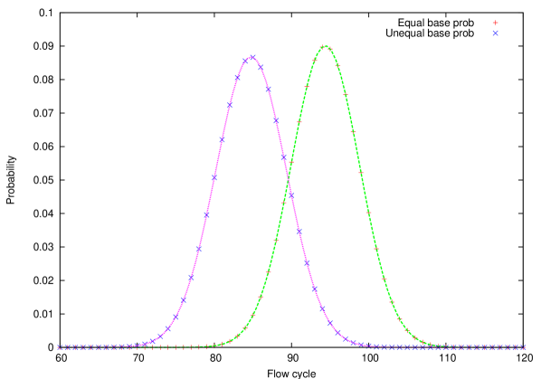
Figure 1: The distributions of flow cycles for a fixed sequence length of $n=250$ base pairs, for both equal nucleotide probability (on the right) and unequal nucleotide probabilities (on the left). The unequal nucleotide probabilities used here are $p_{a}=1/3=0.3333$, $p_{b}=1/11=0.0909$, $p_{c}=100/231=0.4329$, and $p_{d}=1/7=0.1429$. The exact distributions are calculated from Eq. (2.2). The continuous curves are the normal distributions $N({\bar{f}}(n),\sigma_{f}^{2}(n))$ of the same mean and variance as those of the exact distributions, where ${\bar{f}}(n)$ and $\sigma_{f}^{2}(n)$ are calculated from Eqs. (16) and (17). The two normal distributions shown here are $N(94.375,19.609375)$ and $N(84.765278,21.121065)$, for equal and unequal nucleotide probabilities, respectively.

3.2 Fixed flow cycle: distribution of sequence length

When the number of flow cycles $f$ is fixed, the mean ${\bar{n}}(f)$ and variance $\sigma_{n}^{2}(f)$ of the length of the sequences that can be determined by these flow cycles can also be calculated from the exact probability GFs as described in the previous section, by using Eqs 14 and 15:

$${\bar{n}}(f) \approx\frac{f}{s_{2}}+\frac{2s_{3}}{s_{2}^{2}}-2,$$ (20)

$$\sigma_{n}^{2}(f) \approx\frac{s_{2}-3s_{2}^{2}+2s_{3}}{s_{2}^{3}}f-2\frac{3s_{2}s_{4}-4s_{3}^{2}+s_{2}^{2}s_{3}}{s_{2}^{4}}.$$ (21)

As discussed in section 2.3, the small extra terms are ignored in the above expressions. Practically they do not affect any discussions in the following.

From Eqs. (20) and (21) we can see that both the average sequence length ${\bar{n}}(f)$ and the variance $\sigma_{n}^{2}(f)$ increase linearly with the number of flow cycle $f$. When $p_{a}=p_{b}=p_{c}=p_{d}=1/4$, we have

$${\bar{n}}(f) \approx\frac{8}{3}f-\frac{10}{9},$$ (22)

$$\sigma_{n}^{2}(f) \approx\frac{40}{27}f-\frac{20}{81}.$$ (23)

By using the constraint $s_{1}=p_{a}+p_{b}+p_{c}+p_{d}=1$, it can be shown that when the four nucleotides have equal probability, both of the average sequence length and the variance are at their mimima. In other words, for a given number of flow cycles, on average longer read lengths can be achieved when the target sequences have unequal nucleotide probabilities, but the variance is also greater than that of the sequences with equal nucleotide probability.

In Figure 2 the exact distributions of sequence length in base pairs are shown for a fixed number of flow cycles $f=100$ ($400$ nucleotide flows), for both equal nucleotide probability (on the left) and unequal nucleotide probabilities (on the right). The unequal nucleotide probabilities used here are the same as in the previous section. These exact distributions are calculated from Eq. (2.2) in section 2.

Also shown in Figure 2 in continuous curves are the normal distributions $N({\bar{n}}(f),\sigma_{n}^{2}(f))$, the mean ${\bar{n}}(f)$ and variance $\sigma_{n}^{2}(f)$ of which are calculated from Eqs. (20) and (21). Just like the distributions of the number of flow cycles at fixed sequence length as discussed in the previous section, the exact distributions of sequence length at a fixed number of flow cycles can also be approximated quite well with normal distributions with the same mean and variance as those of the exact distributions. For the two examples here, the normal distributions are $N(265.5555556,148.3950617)$ and $N(296.0312085,221.46233357)$, for equal and unequal nucleotide probabilities, respectively.

Compared with the almost perfect fit between the exact and normal distributions in Figure 1, the curves of normal distributions in Figure 2 show some small disagreements with the exact distributions. The difference here is that the exact distributions have a slightly longer tails on the right and a slightly shorter tail on the left when compared to the normal distributions. Intuitively this discrepancies can be understood by the fact that the distributions of sequence length discussed in this section include sequences of all theoretically possible lengths, from the order of $f$ up to infinity. When the sequence length is fixed, as discussed in the previous section, however, there are only finite number of possible flow cycles. For a sequence with length $n$, the number of nucleotide flows is from $1$ to $3n+1$, as discussed previously in section 1.

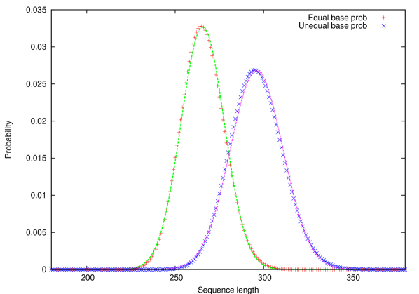
Figure 2: The distributions of sequence length in base pairs for a fixed number of flow cycles $f=100$, for both equal nucleotide probability (on the left) and unequal nucleotide probabilities (on the right). The unequal nucleotide probabilities used here are the same as in Figure 1. The exact distributions are calculated from Eq. (2.2). The continuous curves are the normal distributions $N({\bar{n}}(f),\sigma_{n}^{2}(f))$ with the same mean and variance as those of the exact distributions, where ${\bar{n}}(f)$ and $\sigma_{n}^{2}(f)$ are calculated from Eqs. (20) and (21). The two normal distributions shown here are $N(265.5555556,148.3950617)$ and $N(296.0312085,221.46233357)$, for equal and unequal nucleotide probabilities, respectively.

3.3 Fixed sequence length: distributions of individual nucleotide flows

In the previous two sections we discussed the distributions with regards to the flow cycles, which by definition are the collective behaviors of the flows within the “quad cycle” (see the definitions in Table 1). The advantage to deal with the quad flow cycles instead of the individual nucleotide flows is the symmetry in the expressions: the master GF Eq. (2.2) and the results derived from it (Eqs. (16), (17), (20), and (21)) are symmetric in the nucleotide probabilities $p_{a}$, $p_{b}$, $p_{c}$, and $p_{d}$: these individual probabilities do not appear in the expressions; only the elementary symmetric functions $s_{i}$’s are in the equations. If any two nucleotide probabilities are swapped, the results will not be affected.

In this and the next sections the distributions with respect to the individual nucleotide flows will be presented. Here we discuss explicitly the probabilities that nucleotide flows ending in $a$, $b$, $c$, or $d$ will finish the sequence. For example, the first sample sequence in Table 1 finishes at flow number $12$ at a nucleotide $d$, while the second sample sequence finishes at flow number $7$ at a nucleotide $c$. As expected, the expressions will no longer be symmetric with respect to nucleotide probabilities. We’ll first present the distributions of individual nucleotide flows at fixed sequence length below. They are derived from the GFs listed in the section 2 (Eqs. (4), (5), (6), and (7)). The averages of the number of flow cycles that is required to determine sequences of a length of $n$ with the last nucleotide flow ending in each of the four different nucleotides are:

$${\bar{f}_{a}}(n) =s_{2}n+1-2s_{2}+p_{b}+p_{c}+p_{d},$$

$${\bar{f}_{b}}(n) =s_{2}n+1-2s_{2}+p_{c}+p_{d},$$

$${\bar{f}_{c}}(n) =s_{2}n+1-2s_{2}+p_{d},$$

$${\bar{f}_{d}}(n) =s_{2}n+1-2s_{2},$$ (24)

and the variances

$$\sigma_{f_{a}}^{2} =(2s_{3}-3s_{2}^{2}+s_{2})n+8s_{2}^{2}-6s_{3}-2s_{2}+\sum_{i=b,c,d}(p_{i}-p_{i}^{2}-2p_{i}s_{2}),$$

$$\sigma_{f_{b}}^{2} =(2s_{3}-3s_{2}^{2}+s_{2})n+8s_{2}^{2}-6s_{3}-2s_{2}+\sum_{i=c,d}(p_{i}-p_{i}^{2}-2p_{i}s_{2}),$$

$$\sigma_{f_{c}}^{2} =(2s_{3}-3s_{2}^{2}+s_{2})n+8s_{2}^{2}-6s_{3}-2s_{2}+p_{d}-p_{d}^{2}-2p_{d}s_{2},$$

$$\sigma_{f_{d}}^{2} =(2s_{3}-3s_{2}^{2}+s_{2})n+8s_{2}^{2}-6s_{3}-2s_{2}.$$ (25)

From these expressions we see again that the mean and variance of the distributions vary linearly with the sequence length $n$.

In Figure 3 the exact distributions of flow cycles are shown for the four nucleotides at a fixed sequence length of $n=250$ for unequal nucleotide probabilities in the target sequences. The nucleotide probabilities used here are the same as in the previous sections. These exact distributions are calculated from Eqs. (4), (5), (6), and (7) in section 2. We can see that the magnitudes of the probabilities in the distributions are proportional to the nucleotide frequencies. From $a$ to $d$, the mean shifts to the left slightly, which can be confirmed by Eq. (3.3).

Also shown in Figure 3 in continuous curves are the normal distributions $N({\bar{f}_{i}}(n),\sigma_{f_{i}}^{2}(n))$, for $i=a,b,c,d$, with the same means and variances as those of the exact distributions, calculated from Eqs. (3.3) and (3.3). The normal distributions are multiplied by the normalization factors Eq. (2.3) discussed in section 2. As for the fixed sequence length case with quad cycles discussed previously (Figure 1), the approximations by normal distributions are almost perfect.

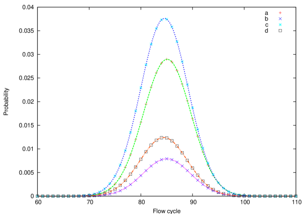
Figure 3: The distributions of individual flow cycles for a fixed sequence length of $n=250$ base pairs. The nucleotide probabilities used here are the same as those in the unequal probability case in Figure 1. These exact distributions are calculated from Eqs. (4), (5), (6), and (7) in section 2. The continuous curves are the normal distributions $N({\bar{f}_{i}}(n),\sigma_{i}^{2}(n))$ with the same means ${\bar{f}_{i}}(n)$ and variances $\sigma_{f_{i}}^{2}(n)$ as those of the exact distributions, which are calculated from Eqs. (3.3) and (3.3) for $i=a,b,c,d$. The normal distributions are scaled by the normalization factors of Eq. (2.3).

3.4 Fixed flow cycle: distributions of sequence length ending with a particular individual nucleotide flow

In this section the mean and variance of sequence length that can be determined at a fixed number of flow cycles with the last nucleotide flow ending at one of the four different nucleotides are given. For the means, we have

$${\bar{n}_{a}}(f) \approx\frac{1}{s_{2}}f-\frac{(p_{b}+p_{c}+p_{d})s_{2}-2s_{3}+s_{2}^{2}}{s_{2}^{2}},$$

$${\bar{n}_{b}}(f) \approx\frac{1}{s_{2}}f-\frac{(p_{c}+p_{d})s_{2}-2s_{3}+s_{2}^{2}}{s_{2}^{2}},$$

$${\bar{n}_{c}}(f) \approx\frac{1}{s_{2}}f-\frac{p_{d}s_{2}-2s_{3}+s_{2}^{2}}{s_{2}^{2}},$$

$${\bar{n}_{d}}(f) \approx\frac{1}{s_{2}}f-\frac{-2s_{3}+s_{2}^{2}}{s_{2}^{2}},$$ (26)

and for the variances,

$$\sigma^{2}_{n_{a}} \approx\frac{2s_{3}-3s_{2}^{2}+s_{2}}{s_{2}^{3}}f-\frac{-8s_{3}^{2}+6s_{4}s_{2}+2s_{2}^{2}s_{3}+{\displaystyle\sum_{i=b,c,d}(p_{i}^{2}s_{2}^{2}-p_{i}s_{2}^{3}+2p_{i}s_{2}s_{3})}}{s_{2}^{4}},$$

$$\sigma^{2}_{n_{b}} \approx\frac{2s_{3}-3s_{2}^{2}+s_{2}}{s_{2}^{3}}f-\frac{-8s_{3}^{2}+6s_{4}s_{2}+2s_{2}^{2}s_{3}+{\displaystyle\sum_{i=c,d}(p_{i}^{2}s_{2}^{2}-p_{i}s_{2}^{3}+2p_{i}s_{2}s_{3})}}{s_{2}^{4}},$$

$$\sigma^{2}_{n_{c}} \approx\frac{2s_{3}-3s_{2}^{2}+s_{2}}{s_{2}^{3}}f-\frac{-8s_{3}^{2}+6s_{4}s_{2}+2s_{2}^{2}s_{3}+p_{d}^{2}s_{2}^{2}-p_{d}s_{2}^{3}+2p_{d}s_{2}s_{3}}{s_{2}^{4}},$$

$$\sigma^{2}_{n_{d}} \approx\frac{2s_{3}-3s_{2}^{2}+s_{2}}{s_{2}^{3}}f-2\frac{-4s_{3}^{2}+3s_{4}s_{2}+s_{2}^{2}s_{3}}{s_{2}^{4}}.$$ (27)

As in section 3.2 for the “quad cycle” distribution of sequence length, the small extra terms in these expressions are not shown here for clarity reason.

In Figure 4 the exact distributions of the length of the sequences that can be determined with $f=100$ flow cycles and with the last flow ending in one of the four different nucleotides are shown. The nucleotide probabilities used here are the same as in the previous sections. These exact distributions are calculated from Eqs. (4), (5), (6), and (7) in section 2.

Also shown in Figure 4 in continuous curves are the normal distributions $N({\bar{n}_{i}}(f),\sigma_{n_{i}}^{2}(f))$, $i=a,b,c,d$, with the same means and variances as those of the exact distributions, calculated from Eqs. (3.4) and (3.4). The normal distributions are multiplied by the normalization factors Eq. (2.3) discussed in section 2. Similar to the quad cycles case with fixed number of cycles discussed previously, the sequence length distributions can be approximated accurately by the normal distributions with the same mean and variance, with slightly longer tails on the right and a slightly short tails on the left for the exact distributions. From $a$ to $d$, the mean shifts to the right slightly, which can be confirmed by Eq. (3.4).

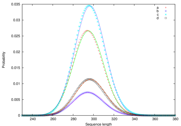
Figure 4: The distributions of of sequence length that can be determined with the number of flow cycles $f=100$, and with the last flow ending in the four different nucleotides. The nucleotide probabilities used here are the same as those in the unequal probability case in Figure 1. These exact distributions are calculated from Eqs. (4), (5), (6), and (7) in section 2. The continuous curves are the normal distributions $N({\bar{n}_{i}}(f),\sigma_{n_{i}}^{2}(f))$ with the same means ${\bar{n}_{i}}(f)$ and variances $\sigma_{n_{i}}^{2}(f)$ as those of the exact distributions, which are calculated from Eqs. (3.4) and (3.4) for $i=a,b,c,d$. The normal distributions are scaled by the normalization factors of Eq. (2.3).

4 Discussion

We have derived the statistical distributions for the pyrosequencing technique, one of the important platforms for the next-generation sequencing technology. Two cases are considered: the distribution of the number of flow cycles for fixed sequence length and the distribution of sequence length for fixed number of flow cycles. In both cases we gave explicit formulas for the mean and variance of the distributions. We demonstrated that these distributions can be approximated accurately by normal distributions with the same mean and variance calculated by the explicit formulas. Both means and variance vary linearly with the number of flow cycles (or sequence length). When the number of flow cycles is fixed, the unequal frequencies of the nucleotides in the target sequences will lead to longer read length with bigger variance (Figure 2); Reciprocally, for a fixed sequence length it will need fewer flow cycles to determine the sequences if the frequencies of the nucleotides in the target sequences are unequal (Figure 1). These explicit formulas and qualitative statements will be useful for instrument and software development of the pyrosequencing platform, and can be used as a guide in monitoring the machine performance for daily users.

References

- Ronaghi et al. (1998) Ronaghi, M., Uhlén, M., and Nyrén, P., 1998. A sequencing method based on real-time pyrophosphate. Science 281, 363–365.
- The PARI Group (2006) The PARI Group, 2006. PARI/GP, version 2.3.3. Bordeaux. Available from http://pari.math.u-bordeaux.fr/.