Exact correlation functions in the cuprate pseudogap phase:
combined effects of charge order and pairing

Abstract

There is a multiplicity of charge ordered, pairing-based or pair density wave theories of the cuprate pseudogap, albeit arising from different microscopic mechanisms. For mean field schemes (of which there are many) we demonstrate here that they have precise implications for two body physics in the same way that they are able to address the one body physics of photoemission spectroscopy. This follows because the full vertex can be obtained exactly from the Ward-Takahashi identity. As an illustration, we present the spin response functions, finding that a recently proposed pair density wave (Amperean pairing) scheme is readily distinguishable from other related scenarios.

Introduction.$-$ A number of theories associated with the cuprate pseudogap phase have recently been suggested, based on now widely observed charge order Saw ; Wise et al. (2008); Comin et al (2014); Hinkov et al. (2007). While the underlying physics may be different, what emerges rather generally are BCS-based pairing theories of the normal state with band-structure reconstruction Chen et al. (2004); Lee (2014); Yang et al. (2006). Distinguishing between theories has mostly been based on angle resolved photoemission spectroscopy (ARPES) Damascelli et al. (2003). However, the majority of data available for the cuprates involves two particle properties: for example, the optical absorption Corson et al. (1999), diamagnetism Li et al. (2010), quasi-particle interference in STM Pan et al. (2000), neutron Stock et al. (2004); Dai et al. (1999); Hinkov et al. (2007) and inelastic x-ray scattering in the charge Comin et al (2014) and spin Tacon et al (2011) sectors.

In this paper we use the Ward-Takahashi identity (WTI) Ryder (1996); Schrieffer (1964) to develop precise two body response functions for these pairing based pseudogap theories. Such exact response functions make it possible to address two particle cuprate experiments, including the list above, from the perspective of many different theories. As an illustration, we compute the spin-spin correlation functions relevant to neutron scattering in three pseudogap scenarios. That the response functions analytically satisfy the $f$-sum rule provides the confidence that there are no missing Feynman diagrams or significant numerical inaccuracies.

By comparing the Amperean pairing scheme Lee (2014), and that of Yang, Rice and Zhang Yang et al. (2006) with a simple $d$-wave pseudogap scenario, we find that the Amperean theory leads to a relatively featureless neutron cross section in contrast to the peaks (at and near the antiferromagnetic wave vector), found for the other two theories.

In this Amperean pairing scheme Lee (2014) the mean field self energy is

$$\Sigma_{pg}(K) =\frac{\Delta_{1}^{2}}{\omega+\xi_{\mathbf{k-p}}-\frac{\Delta_{2}^{2}}{\omega-\xi_{\mathbf{k}-2\mathbf{p}}}}+\frac{\Delta_{2}^{2}}{\omega+\xi_{\mathbf{k+p}}-\frac{\Delta_{1}^{2}}{\omega-\xi_{\mathbf{k}+2\mathbf{p}}}}+\frac{C_{1}^{2}}{\omega-\xi_{\mathbf{k}+2\mathbf{p}}-\frac{\Delta_{1}^{2}}{\omega+\xi_{\mathbf{k+p}}}}+\frac{C_{2}^{2}}{\omega-\xi_{\mathbf{k}-2\mathbf{p}}-\frac{\Delta_{2}^{2}}{\omega+\xi_{\mathbf{k-p}}}}$$

$$+\frac{2\Delta_{1}\Delta_{2}C_{1}}{\left(\omega+\xi_{\mathbf{k+p}}\right)\left(\omega-\xi_{\mathbf{k+2p}}\right)-\Delta_{1}^{2}}+\frac{2\Delta_{1}\Delta_{2}C_{2}}{\left(\omega+\xi_{\mathbf{k-p}}\right)\left(\omega-\xi_{\mathbf{k-2p}}\right)-\Delta_{2}^{2}}.$$ (1)

We single this particular theory out as an example which is complex and therefore somewhat more inclusive. In Eq. (Exact correlation functions in the cuprate pseudogap phase: combined effects of charge order and pairing) $\Sigma_{pg}(K)$ is expressed in terms of two different finite momentum ($\mathbf{p}$) pseudogaps, $\Delta_{1}\equiv\Delta_{\mathbf{p}}$ and $\Delta_{2}\equiv\Delta_{-\mathbf{p}}$. In addition we have introduced charge density wave (CDW) amplitudes $C_{1}\equiv C_{2\mathbf{p}}$ and $C_{2}\equiv C_{-2\mathbf{p}}$. From the self energy, the full (inverse) Green’s function can be deduced: $G^{-1}(K)\equiv G_{0}^{-1}(K)-\Sigma_{pg}(K)=\omega-\xi_{\mathbf{k}}-\Sigma_{pg}(K)$. This then determines the renormalized band-structure, which can be compared with ARPES experiments. One can similarly add other mean field contributions such as that related to an SDW Podolsky et al. (2003) or even a DDW Chakravarty et al. (2001).

It is observed from Eq. (Exact correlation functions in the cuprate pseudogap phase: combined effects of charge order and pairing) that in the Amperean pairing case a BCS-like self energy appears in a continued fraction form within the self energy itself. There are analogies with the approach of Yang, Rice and Zhang (YRZ) Yang et al. (2006) in the limit that only one gap term is present, say $\Delta_{1}$, and when the CDW ordering is absent. Importantly, this single gap self energy involves two types of dispersion relations, so that the pairing term leads to pockets or a reconstruction of the band-structure. For a simpler $d$-wave pseudogap, with a single gap model, both of these dispersion relations are taken to be the same, as was studied microscopically Chen et al. (2005) and phenomenologically Norman et al. (1998). A central contribution of this paper is to show how, via two particle properties, important distinctions between these three different pseudogap theories can be established.

While it is argued to be appropriate for the pseudogap phase Lee (2014), the self energy of Eq. (Exact correlation functions in the cuprate pseudogap phase: combined effects of charge order and pairing) is indistinguishable from that of a superconducting state. It is important, then, to ensure that this form for $\Sigma_{pg}$ does not correspond to an ordered phase. Phase fluctuations have been phenomenologically invoked Chen et al. (2004); Lee (2014) to destroy order. Regardless of this phenomenology there is a quantitative constraint to be satisfied: the absence of a Meissner effect above $T_{C}$ implies that the zero frequency and zero momentum current-current correlation function satisfies $-\tensor{P}(0)=\left(\tensor{\frac{n}{m}}\right)_{\rm dia}\equiv 2\sum_{K}\frac{\partial^{2}\xi_{\mathbf{k}}}{\partial{\mathbf{k}}\partial{\mathbf{k}}}G(K)$, so that there is a precise cancellation between the diamagnetic and paramagnetic current-current correlation functions in the normal state.

Performing integration by parts dis and using the identity $\partial G(K)/\partial\mathbf{k}=-G^{2}(K)\partial G^{-1}(K)/\partial\mathbf{k}$ then yields the following expression for $\tensor{P}(0)$:

$$\tensor{P}(0)=2\sum_{K}G^{2}(K)\biggl{\{}\frac{\partial\xi_{\mathbf{k}}}{\partial\mathbf{k}}+\frac{\partial\Sigma_{pg}(K)}{\partial\mathbf{k}}\biggr{\}}\frac{\partial\xi_{\mathbf{k}}}{\partial\mathbf{k}}.$$ (2)

Here $K=(\omega,\mathbf{k})$. Given the self energy from Eq. (Exact correlation functions in the cuprate pseudogap phase: combined effects of charge order and pairing), it is then straightforward to arrive at the quantity $\tensor{P}(0)$:

$$\tensor{P}(0)=2\sum_{K}G^{2}(K)\biggl{\{}\frac{\partial\xi_{\mathbf{k}}}{\partial\mathbf{k}}-\Delta^{2}_{1}G^{2}_{1,1}(-K)\frac{\partial\xi_{\mathbf{k},2}}{\partial\mathbf{k}}$$

$$+\Delta^{2}_{1}\Delta^{2}_{2}G^{2}_{1,1}(-K)G^{2}_{0,4}(K)\frac{\partial\xi_{\mathbf{k},4}}{\partial\mathbf{k}}-\Delta^{2}_{2}G^{2}_{1,2}(-K)\frac{\partial\xi_{\mathbf{k},1}}{\partial\mathbf{k}}$$

$$+\Delta^{2}_{2}\Delta^{2}_{1}G^{2}_{1,2}(-K)G^{2}_{0,3}(K)\frac{\partial\xi_{\mathbf{k},3}}{\partial\mathbf{k}}\biggr{\}}\frac{\partial\xi_{\mathbf{k}}}{\partial\mathbf{k}}.$$ (3)

For simplicity, throughout the main text we set $C_{1}=C_{2}=0$ and present the complete expressions in the Supplemental Material. Here we have defined the following four bare (inverse) Green’s functions $G^{-1}_{0,i}(K)=(\omega-\xi_{\mathbf{k},i}),\quad i\in\{1,2,3,4\}$, where $\xi_{\mathbf{k},1}=\xi_{\mathbf{k+p}}$, $\xi_{\mathbf{k},2}=\xi_{\mathbf{k-p}}$, $\xi_{\mathbf{k},3}=\xi_{\mathbf{k}+2\mathbf{p}}$, $\xi_{\mathbf{k},4}=\xi_{\mathbf{k}-2\mathbf{p}}$ are four dispersion relations. (The usual bare inverse Green’s function is denoted by $G^{-1}_{0}(K)=\omega-\xi_{\mathbf{k}}=\omega-\epsilon_{\mathbf{k}}+\mu$.) The partially dressed Green’s functions (which are neither bare nor full) associated with Eq. (Exact correlation functions in the cuprate pseudogap phase: combined effects of charge order and pairing) are

$$G^{-1}_{1,1}(K) ={\omega-\xi_{\mathbf{k},1}}-\frac{\Delta_{2}^{2}}{\omega+\xi_{-\mathbf{k},4}},$$ (4)

$$G^{-1}_{1,2}(K) ={\omega-\xi_{\mathbf{k},2}}-\frac{\Delta_{1}^{2}}{\omega+\xi_{-\mathbf{k},3}}.$$ (5)

In terms of these partially dressed Green’s functions the self energy in Eq. (Exact correlation functions in the cuprate pseudogap phase: combined effects of charge order and pairing) for the case where $C_{1}=C_{2}=0$ has the compact form $\Sigma_{pg}(K)=-\Delta^{2}_{1}G_{1,1}(-K)-\Delta^{2}_{2}G_{1,2}(-K)$. The quantity $\tensor{P}(0)$ in Eq. (Exact correlation functions in the cuprate pseudogap phase: combined effects of charge order and pairing) provides a template for the form of the Feynman diagrams that we will find in $\tensor{P}(Q)$.

Ward-Takahashi identity (WTI) for the full vertex.$-$ The exact expression for the current-current correlation function, $\tensor{P}(Q)$, is contained in the response functions written as

$$P^{\mu\nu}(Q)=2\sum_{K}\Gamma^{\mu}(\widetilde{K},K)G(K)\gamma^{\nu}(K,\widetilde{K})G(\widetilde{K}).$$ (6)

Throughout the text, we set $\widetilde{K}\equiv K+Q$. The full vertex in four-vector notation is given by $\Gamma^{\mu}(\widetilde{K},K)=(\Gamma^{0}(\widetilde{K},K),\boldsymbol{\Gamma}(\widetilde{K},K))$, where the first argument denotes the incoming momentum and the second argument, the outgoing momentum. Here the quantity $\gamma^{\nu}(K,\widetilde{K})$ represents the bare vertex.

The full response kernel is $K^{\mu\nu}(Q)\equiv P^{\mu\nu}(Q)+\left({\tfrac{n}{m}}\right)^{\mu\nu}_{\rm dia}(1-\delta_{0,\nu}\delta_{\mu,\nu}),$ where there is no summation over indices in the second term. The Ward-Takahashi identity in quantum field theory is a diagrammatic identity that imposes a symmetry between response functions. The particular symmetry we are interested in is the $\rm U(1)_{EM}$ abelian gauge symmetry Ryder (1996). As we shall show, satisfying the WTI also leads to manifestly sum rule consistent response functions. Charge conservation is an exact relation between the current-current and density-density response functions that follows from this $\rm U(1)_{EM}$ symmetry. The WTI reflects this charge conservation which imposes the constraint: $\Omega K^{0\nu}+i\mathrm{div}_{\mathbf{q}}K^{j\nu}=0.$ The WTI, for the vertex $\Gamma^{\mu}(\widetilde{K},K)$, on a lattice is

$$\Omega\Gamma^{0}(\widetilde{K},K)+i\mathrm{div}_{\mathbf{q}}\boldsymbol{\Gamma}(\widetilde{K},K)$$

$$=G^{-1}(\widetilde{K})-G^{-1}(K),$$

$$=\Omega+i\mathrm{div}_{\mathbf{q}}\boldsymbol{\gamma}(\widetilde{K},K)+\Sigma_{pg}(K)-\Sigma_{pg}(\widetilde{K}).$$ (7)

The WTI for the bare vertex $\gamma^{\mu}(\widetilde{K},K)$ is $\Omega+i\mathrm{div}_{\mathbf{q}}\boldsymbol{\gamma}=G^{-1}_{0}(\widetilde{K})-G^{-1}_{0}(K)=\Omega-\xi_{\mathbf{k+q}}+\xi_{\mathbf{k}}$. Similarly we introduce the bare vertices $\gamma^{\mu}_{i}(\widetilde{K},K)$ associated with the dispersion relations $\xi_{\mathbf{k},i}$. Here $\mathrm{div}_{\mathbf{q}}\boldsymbol{\Gamma}(\widetilde{K},K)$, complicated due to lattice effects, is the Fourier transform of the divergence of $\boldsymbol{\Gamma}$.

In the limit $Q\rightarrow 0$, the Ward-Takahashi identity reduces to the Ward identity: $\delta\Gamma^{\mu}(K,K)\equiv\Gamma^{\mu}(K,K)-\gamma^{\mu}(K,K)=-\partial\Sigma_{pg}(K)/\partial k_{\mu}.$ This is fully consistent with the arguments leading up to the no-Meissner constraint in Eq. (2). In this continuum limit, ($q\rightarrow 0$) the WTI and charge conservation have familiar forms: $q_{\mu}\Gamma^{\mu}(\widetilde{K},K)=G^{-1}(\widetilde{K})-G^{-1}(K)$ and $q_{\mu}K^{\mu\nu}(Q)=0$.

We emphasize that, given an arbitrary self energy, solving the WTI analytically for the full vertex $\Gamma^{\mu}(\widetilde{K},K)$ is generally not possible. However, there is a well-defined procedure to determine this vertex in principle. One inserts the bare vertex in all possible places in the self energy diagram and sums the resulting series of diagrams. For the class of theories considered in this paper $\Sigma$ itself does not depend on the full Green’s function $G(\Sigma)$, but rather depends on the bare Green’s functions $G_{0}$ and their simple extensions; this is associated with generalized mean field theories. For example, in strict BCS theory $\Sigma(K)=-\Delta^{2}G_{0}(-K)$.

Importantly, it follows that in the BCS-like theories of interest here, the full vertex, $\Gamma^{\mu}(\widetilde{K},K)$, can be deduced from the equivalent WTI by considering only finitely many loop diagrams. We illustrate this procedure specifically for the first term in the Amperean self energy in Eq. (Exact correlation functions in the cuprate pseudogap phase: combined effects of charge order and pairing). Using the form of the self energy, along with the bare WTI, we have: $\Sigma_{1}(K)-\Sigma_{1}(\widetilde{K})$

$$=\Delta^{2}_{1}G_{1,1}(-K)G_{1,1}(-\widetilde{K})\{[\Omega+\xi_{\mathbf{k+q-p}}-\xi_{\mathbf{k-p}}]$$

$$+\Delta^{2}_{2}G_{0,4}(K)G_{0,4}(\widetilde{K})[\Omega-\xi_{\mathbf{k+q}-2\mathbf{p}}+\xi_{\mathbf{k}-2\mathbf{p}}]\}$$

$$=\Delta^{2}_{1}G_{1,1}(-K)G_{1,1}(-\widetilde{K})\{[\Omega+i\mathrm{div}_{\mathbf{q}}\boldsymbol{\gamma}_{1}(-K,-\widetilde{K})]$$

$$+\Delta^{2}_{2}G_{0,4}(K)G_{0,4}(\widetilde{K})[\Omega+i\mathrm{div}_{\mathbf{q}}\boldsymbol{\gamma}_{4}(\widetilde{K},K)]\}.$$ (8)

and $\Omega\Gamma^{0}(\widetilde{K},K)+i\mathrm{div}_{\mathbf{q}}\boldsymbol{\Gamma}=$

$$\Omega+i\mathrm{div}_{\mathbf{q}}\boldsymbol{\gamma}+\Delta^{2}_{1}G_{1,1}(-K)G_{1,1}(-\widetilde{K})$$

$$\times\{[\Omega+i\mathrm{div}_{\mathbf{q}}\boldsymbol{\gamma}_{1}(-K,-\widetilde{K})]$$

$$+G_{0,4}(K)G_{0,4}(\widetilde{K})[\Omega+i\mathrm{div}_{\mathbf{q}}\boldsymbol{\gamma}_{4}(\widetilde{K},K)]\}.$$ (9)

In this form we can then solve for the exact full vertex

$$\Gamma^{\mu}(\widetilde{K},K)=\gamma^{\mu}(\widetilde{K},K)+\Delta^{2}_{1}G_{1,1}(-K)G_{1,1}(-\widetilde{K})$$

$$\times[\gamma^{\mu}_{1}(-K,-\widetilde{K})+\Delta^{2}_{2}G_{0,4}(K)G_{0,4}(\widetilde{K})\gamma^{\mu}_{4}(\widetilde{K},K)]$$

$$+\Delta^{2}_{2}G_{1,2}(-K)G_{1,2}(-\widetilde{K})$$

$$\times[\gamma^{\mu}_{2}(-K,-\widetilde{K})+\Delta^{2}_{1}G_{0,3}(K)G_{0,3}(\widetilde{K})\gamma^{\mu}_{3}(\widetilde{K},K)].$$ (10)

Here we have now included the second term from $\Sigma_{pg}(K)$ in Eq. (Exact correlation functions in the cuprate pseudogap phase: combined effects of charge order and pairing).

We emphasize this is not an expansion in the bare vertices. Rather, the WTI is used to obtain the exact full vertex. The crucial step is that the self energy does not depend on the full Green’s function. If it did, then the full vertex would appear on both sides of the equation, reducing the problem to a Bethe-Salpeter equation Schrieffer (1964).

Using the full vertex, the exact response function can then be determined via Eq. (6). The Amperean pairing response functions have twenty one associated Feynman diagrams if one considered the charge density wave: one of one loop order (two Green’s functions), four of two loop order (four Green’s functions), and four of three loop order (six Green’s functions), plus an additional twelve diagrams with an odd number of Green’s functions. The twenty one Feynman diagrams contributing to the response functions are presented in the Supplemental Material.

The bare vertices for the density component are given by $\gamma^{0}(\widetilde{K},K)=\gamma^{0}_{i}(\widetilde{K},K)=1$. This then allows the exact density-density response function $P_{\rho\rho}(Q)$ to be computed for all $Q$. More complicated, for an arbitrary band-structure, are the bare vertices that enter into the current-current correlation function. However, in the limit $q\rightarrow 0$ these can be determined from Eq. (Exact correlation functions in the cuprate pseudogap phase: combined effects of charge order and pairing). The same reasoning which is used to determine $P_{\rho\rho}(Q)$ for all $Q$ is applicable to the spin (density) response, as measured in neutron experiments.

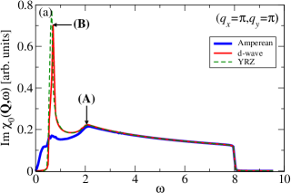
(a)

(b)

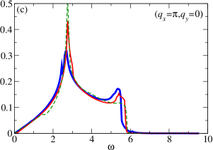
(c)

Figure 1: Comparison of the spin density correlation function $\mathrm{Im}\chi_{0}(Q)=-\mathrm{Im}P^{00}_{S}(\mathbf{q},\omega)$ for three different values of $\mathbf{q}$ in the Amperean, $d$-wave and YRZ pseudogap theories. In (a) we have labeled the Van Hove peaks appearing in the $d$-wave theory, which appear as saddle points in the contour plot of Fig. (2). Here we use the band structure given in Comin et al (2014) with $T=0.01$ and a broadening of $\Gamma=0.01$. The doping $p=0.12$ and the chemical potential $\mu$ is fixed by the Luttinger sum rule. The band-structure and frequency are all normalized by $t$, and the gap function has an amplitude of $\Delta_{0}=0.15$. For the Amperean theory we use a $k_{x},k_{y}$-symmetrized Gaussian Lee (2014) gap function.

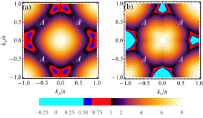
(a)

Figure 2: The equal energy contours $E_{2}(\mathbf{k})\equiv E_{\mathbf{k}}+E_{\mathbf{k+q}}$ which appear as the integrand in $\mathrm{Im}\chi_{0}(\mathbf{q},\omega)$ for both (a) $\it d$-wave and (b) the Amperean pseudogap schemes. Here $\mathbf{q}=(\pi,\pi)$. Note there are several energy scales as indicated by the legend. The labels $A$ and $B$ indicate the location of the saddle points of $\mathrm{Im}\chi_{0}(\mathbf{q},\omega)$.

The full spin response function $P^{\mu\nu}_{S}(Q)$ is defined by

$$P^{\mu\nu}_{S}(Q)=\sum_{K}\sum_{\sigma}\Gamma^{\mu}_{S_{\sigma}}(\widetilde{K},K)G(K)\gamma^{\nu}_{S_{\sigma}}(K,\widetilde{K})G(\widetilde{K}).$$ (11)

Here the bare spin vertex is denoted by $\gamma^{\mu}_{S_{\sigma}}(\widetilde{K},K)$, where $S_{\sigma}=\pm 1$ and $S_{\bar{\sigma}}=-S_{\sigma}$. The bare WTI for the spin vertex is $\Omega+i\mathrm{div}_{\mathbf{q}}\boldsymbol{\gamma}_{S_{\sigma}}=S_{\sigma}(G^{-1}_{0}(\widetilde{K})-G^{-1}_{0}(K))=S_{\sigma}(\Omega-\xi_{\mathbf{k+q}}+\xi_{\mathbf{k}})$. Similarly the full WTI for the full spin vertex $\Gamma^{\mu}_{S_{\sigma}}(\widetilde{K},K)$ is

$$\Omega\Gamma^{0}_{S_{\sigma}}+i\mathrm{div}_{\mathbf{q}}\boldsymbol{\Gamma}_{S_{\sigma}}=S_{\sigma}(G^{-1}(\widetilde{K})-G^{-1}(K)).$$ (12)

We can then read off the spin-spin correlation function directly using Eq. (10).

From the established constraints on the bare and full vertices one can directly derive Bergeron et al. (2011) the $f$-sum rule for the density-density and spin density response functions:

$$\int\frac{d\omega}{\pi}(-\omega\mathrm{Im}P^{00}(Q))=2\sum_{\mathbf{k}}n_{\mathbf{k}}[\xi_{\mathbf{k+q}}+\xi_{\mathbf{k-q}}-2\xi_{\mathbf{k}}],$$ (13)

where $n_{\mathbf{k}}=T\sum_{i\omega}G(K).$ Importantly, this sum rule (and counterparts for the current-current correlation function) are satisfied exactly providing the response functions are consistent with the WTI. This is discussed in more detail in the Supplemental Material.

Behavior of the neutron cross section: Comparison of Pseudogap theories.$-$ For illustrative purposes we focus on the spin-density response function, conventionally called $\chi_{0}(Q)$. Importantly, ensuring Eq. (13) is satisfied provides tight control over numerical calculations of this correlation function. When no simplifications are introduced, our numerical calculations agree with the sum rule to an accuracy of the order of $0.1-0.2$ percent dis in all three models. The quantity $\mathrm{Im}\chi_{0}(Q)\equiv-\mathrm{Im}P^{00}(Q)$ is the theoretical basis for neutron scattering experiments. [Note we adopt the sign convention for the density correlation functions, $P_{\rho\rho}(Q)=P^{00}(Q)$ for spin and charge.]

For simple $d$-wave pairing models, a very reasonable comparison between theory and neutron data has been reported at high temperatures (where one sees a reflection of the fermiology Si et al. (1993); Zha et al. (1993a)) and below $T_{C}$ (where one sees both commensurate ($\pi,\pi$) Liu et al. (1995) and slightly incommensurate frequency dependent “hourglass” structure Zha et al. (1993b); Kao et al. (2000)). This approach to neutron scattering presents a (rather successful) rival scheme to stripe approaches; many different theories, built on different microscopics, have arrived at similar behavior Stemmann et al. (1994); Brinckmann and Lee (1999); Norman (2000); James et al. (2012). In the pseudogap phase (which has received less attention theoretically), there are peaks at and near ($\pi,\pi$) Stock et al. (2004); Dai et al. (1999); Hinkov et al. (2007) which have been recently argued Hinkov et al. (2007) to reflect some degree of broken orientational symmetry.

Here we compare the results for $\chi_{0}(Q)$ using three different theories of the pseudogap: a simple $d$-wave pseudogap, the theory of Yang, Rice and Zhang, and that of Amperean pairing. For the Amperean case we follow Lee (2014) and consider the simpler $3\times 3$ reduced Hamiltonian. In this $3\times 3$ form, $C_{1}=C_{2}=0$ and terms involving $\xi_{\mathbf{k}\pm 2\mathbf{p}}$ are dropped. We do not include the effects of the widely used RPA enhanced denominator introduced in Si et al. (1992). In the RPA enhanced form $\chi(Q)=\chi_{0}(Q)/[1+J(Q)\chi_{0}(Q)]$, where $J(Q)$ is an effective exchange. Even though $\chi_{0}(Q)$ is exact, introducing this ratio will lead to a violation of the $f$-sum rule; this effect is not central to distinguishing between theories, as is our goal here.

Figure (1) presents a plot of $\mathrm{Im}\chi_{0}(Q)$, for three fixed $\mathbf{q}$ corresponding to ($\pi,\pi)$ in (a), ($\pi,0.75\pi$) in (b) and ($\pi,0$) in (c) as functions of $\omega$. The normal state (above $T^{*}$) band-structure is taken to be the same, as is the pseudogap amplitude. The behavior in the low $\omega$ regime is principally, but not exclusively, dominated by the effects of the gap, while at very high $\omega$ the behavior is band-structure dominated. Importantly, all theories essentially converge once $\omega$ is much larger than the gap. This means that interesting effects associated with high energy scales Tacon et al (2011) such as observed in recent RIXS experiments, would not be specific to a given theory.

Figure (1) shows that there is little difference in the spin dynamics between the approach of YRZ Yang et al. (2006) and that of a $d$-wave pseudogap, emphasized earlier in a different context Scherpelz et al. (2014) and helps to explain the literature claims of successful reconciliation with the data that surround both scenarios James et al. (2012); Zha et al. (1993b); Kao et al. (2000).

What appears most distinctive is the Amperean pairing response function, particularly away from $\mathbf{q}=(\pi,0)$. Notable here is the absence of the sharp Van Hove peak (marked by $B$ in Fig. (1)) which appears in both other theories and which is ultimately responsible for commensurate peaks or neutron resonance effects Liu et al. (1995). Also missing from the Amperean scenario is the so-called spin-gap, apparent at $(\pi,\pi)$ in both the other two theories. Rather, for Amperean pairing there are multiple low energy processes which contribute to the spin density correlation function.

To better understand these processes, in Fig. (2) we probe the dominant component of the integrand in $\mathrm{Im}\chi_{0}(Q)$ near $\mathbf{q}=(\pi,\pi)$ for the Amperean (right) as compared with $d$-wave pseudogap (left) scenarios. We show the equal energy contours for the sum of the quasi-particle dispersions: $E_{2}(\mathbf{k})\equiv E_{\mathbf{k}}+E_{\mathbf{k+q}}$, vs $k_{x}$ and $k_{y}$ in the pseudogap state e2k . Indicated on the figure are the Van Hove singularities $A$ and $B$ (saddle points in the contour plot), as labeled in Fig. (1a). The lower energy Van Hove point (point $B$) is clearly suppressed in the Amperean pairing case, while it is very pronounced and found to be important Kao et al. (2000) for the $d$-wave case. Also evident from the cyan region in Fig. (2) is the absence of a low $\omega$ minimum (spin gap) in $E_{2}({\bf k})$, as found in both the other two theories, as well as in the integrated response function.

Conclusions.$-$ The central contribution of this paper has been to establish an analytically and numerically controlled methodology for addressing the long list of two particle cuprate measurements. Given a mean field like self energy, the exploitation of the Ward Takahashi identity (and related sum rules) allows one to evaluate two particle properties, and in this way achieve the same level of accuracy in these comparisons, as in, say, ARPES. To demonstrate the utility of this method, we address the spin density response functions of neutron scattering and have singled out signatures of the recently proposed Amperean pairing theory Lee (2014). We cannot firmly establish that this pair density wave theory is inconsistent with experiments (without digressing from our goals and including the sum-rule-inconsistent RPA enhancement denominator Si et al. (1992)), but it does lead to a rather featureless neutron cross section gen . We report two distinctive observations: the absence of both spin gap effects and of the sharp Van Hove peaks near $(\pi,\pi)$.

This work is supported by NSF-MRSEC Grant 0820054. We are grateful to A.-M. S. Tremblay, Yan He and Adam Rançon for helpful conversations.

See pages 1 of Supplemental_Material.pdf See pages 2 of Supplemental_Material.pdf See pages 3 of Supplemental_Material.pdf See pages 4 of Supplemental_Material.pdf See pages 5 of Supplemental_Material.pdf See pages 6 of Supplemental_Material.pdf See pages 7 of Supplemental_Material.pdf

References

- (1) G. Ghiringhelli et al, Science 337, 821 (2012).
- Wise et al. (2008) W. D. Wise, M. C. Boyer, K. Chatterjee, T. Kondo, T. Takeuchi, H. Ikuta, Y. Wang, and E. W. Hudson, Nature Physics 4, 696 (2008).
- Comin et al (2014) R. Comin et al, Science 343, 390 (2014).
- Hinkov et al. (2007) V. Hinkov, P. Bourges, S. Pailhs, Y. Sidis, A. Ivanov, C. D. Frost, T. G. Perring, C. T. Lin, D. P. Chen, and B. Keimer, Nature Physics 3, 780 (2007).
- Chen et al. (2004) H.-D. Chen, O. Vafek, A. Yazdani, and S.-C. Zhang, Phys. Rev. Lett. 93, 187002 (2004).
- Lee (2014) P. A. Lee, Phys. Rev. X 4, 031017 (2014).
- Yang et al. (2006) K.-Y. Yang, T. M. Rice, and F.-C. Zhang, Phys. Rev. B 73, 174501 (2006).
- Damascelli et al. (2003) A. Damascelli, Z. Hussain, and Z.-X. Shen, Rev. Mod. Phys. 75, 473 (2003).
- Corson et al. (1999) J. Corson, R. Mallozzi, J. Orenstein, J. N. Eckstein, and I. Bozovic, Nature 398, 221 (1999).
- Li et al. (2010) L. Li, Y. Wang, S. Komiya, S. Ono, Y. Ando, G. D. Gu, and N. P. Ong, Phys. Rev. B 81, 054510 (2010).
- Pan et al. (2000) S. H. Pan, E. W. Hudson, A. K. Gupta, K.-W. Ng, H. Eisaki, S. Uchida, and J. C. Davis, Phys. Rev. Lett. 85, 1536 (2000).
- Stock et al. (2004) C. Stock, W. J. L. Buyers, R. Liang, D. Peets, Z. Tun, D. Bonn, W. N. Hardy, and R. J. Birgeneau, Phys. Rev. B 69, 014502 (2004).
- Dai et al. (1999) P. Dai, H. A. Mook, S. M. Hayden, G. Aeppli, T. G. Perring, R. D. Hunt, and F. Doan, Science 284, 1344 (1999).
- Tacon et al (2011) M. L. Tacon et al, Nature Physics 7, 725 (2011).
- Ryder (1996) L. H. Ryder, Quantum Field Theory (Cambridge University Press, 1996), 2nd ed.
- Schrieffer (1964) J. R. Schrieffer, Theory of Superconductivity (W.A. Benjamin, Inc., 1964), 1st ed.
- Podolsky et al. (2003) D. Podolsky, E. Demler, K. Damle, and B. I. Halperin, Phys. Rev. B 67, 094514 (2003).
- Chakravarty et al. (2001) S. Chakravarty, R. B. Laughlin, D. K. Morr, and C. Nayak, Phys. Rev. B 63, 094503 (2001).
- Chen et al. (2005) Q. J. Chen, J. Stajic, S. N. Tan, and K. Levin, Phys. Rep. 412, 1 (2005).
- Norman et al. (1998) M. R. Norman, M. Randeria, H. Ding, and J. C. Campuzano, Phys. Rev. B 57, 11093(R) (1998).
- (21) For simplicity in the text, we will ignore terms that arise from the wave vector dependence of the -wave gap function. In general this is a small effect. We can see via the sum rule accuracy the importance of including the full wave vector dependence of the -wave gap. When the wave vector dependence of the gap is ignored, the sum rule accuracy is still very good, but now of the order of 2-3 percent.
- Bergeron et al. (2011) D. Bergeron, V. Hankevych, B. Kyung, and A.-M. S. Tremblay, Phys. Rev. B 84, 085128 (2011).
- Si et al. (1993) Q. Si, Y. Zha, K. Levin, and J. P. Lu, Phys. Rev. B 47, 9055 (1993).
- Zha et al. (1993a) Y. Zha, Q. Si, and K. Levin, Physica C 212, 413 (1993a).
- Liu et al. (1995) D. Z. Liu, Y. Zha, and K. Levin, Phys. Rev. Lett. 75, 4130 (1995).
- Zha et al. (1993b) Y. Zha, K. Levin, and Q. Si, Phys. Rev. B 47, 9124 (1993b).
- Kao et al. (2000) Y.-J. Kao, Q. M. Si, and K. Levin, Phys. Rev. B 61, R118980 (2000).
- Stemmann et al. (1994) G. Stemmann, C. Ppin, and M. Lavagna, Phys. Rev. B 50, 4075 (1994).
- Brinckmann and Lee (1999) J. Brinckmann and P. A. Lee, Phys. Rev. Lett. 82, 2915 (1999).
- Norman (2000) M. R. Norman, Phys. Rev. B 61, 14751 (2000).
- James et al. (2012) A. J. A. James, R. M. Konik, and T. M. Rice, Phys. Rev. B 86, 100508(R) (2012).
- Si et al. (1992) Q. Si, J. P. Lu, and K. Levin, Phys. Rev. B. 45, 4930 (1992).
- Scherpelz et al. (2014) P. Scherpelz, A. Rançon, Y. He, and K. Levin, Phys. Rev. B 90, 060506(R) (2014).
- (34) For the 3 3 Amperean theory, we chose the top band for both and .
- (35) In addition to the gaussian gap model of Ref. Lee (2014), we have found similar featureless results for a simple -wave gap shape as well.