Abstract

I present a calculation of next-to-next-to-next-to-leading-order (NNNLO) soft-gluon corrections for differential distributions in top-antitop pair production in hadronic collisions. Approximate NNNLO (aNNNLO) results are obtained from soft-gluon resummation. Theoretical predictions are shown for the top-quark aNNNLO transverse momentum ($p_{T}$) and rapidity distributions at LHC and Tevatron energies. The aNNNLO corrections enhance previous results for the distributions but have smaller theoretical uncertainties.

1 Introduction

Top quark physics occupies a central role in particle theory and experiment. The top quark has a unique position as the most massive elementary particle to have been discovered, and as the only quark that decays before it can hadronize. Thus understanding the properties and production rates of the top quark in the Standard Model is crucial for QCD, electroweak and Higgs physics, and in searches for new physics.

The production of top quarks can happen either via top-antitop pair production or via single-top production. While the total cross section is the simplest quantity to be calculated and measured, differential distributions provide more detailed information on the production processes. The top-quark transverse momentum ($p_{T}$) and rapidity distributions are particularly useful for discriminating signals of new physics. They have been measured at the Tevatron [1, 2] and the LHC [3, 4] and are in excellent agreement with approximate NNLO (aNNLO) calculations for the $p_{T}$ [5] and rapidity [6] distributions (see also [7] for updates). These aNNLO calculations are based on the resummation of soft-gluon contributions in the double-differential cross section at next-to-next-to-leading-logarithm (NNLL) accuracy in the moment-space approach in perturbative QCD [5, 6, 7]. For a review of resummation in various approaches for top quark production see the review paper in [8]. The theoretical and experimental status of top quark physics has also been more recently reviewed in [9, 10, 11, 12].

The increasing precision of the measurements at the LHC and the upcoming run at 13 TeV necessitate ever more precise theoretical calculations. For the total cross section the current state-of-the-art is approximate NNNLO (aNNNLO) [13]. The purpose of the present paper is to bring the calculation of the top-quark differential distributions to the same accuracy as the total cross section in [13]. The resummation formalism for $t{\bar{t}}$ production has already been presented and discussed extensively in Refs. [5-8,13,14] and we refer the reader to those papers for more details and further references. The accuracy, stability, and reliability of the resummation formalism that we use has been amply demonstrated and discussed in [5, 7]; the soft-gluon corrections approximate exact results for total cross sections and differential distributions at the per mille accuracy level.

In Section 2 we present some details of the formalism and kinematics. In Section 3 we present the top-quark $p_{T}$ distributions at LHC and Tevatron energies. Section 4 contains the corresponding top-quark rapidity distributions. We conclude in Section 5.

2 Soft-gluon corrections and kinematics for differential distributions

At leading order in the strong coupling, $\alpha_{s}$, for $t{\bar{t}}$ production, i.e. ${\cal O}(\alpha_{s}^{2})$, the partonic channels are quark-antiquark annihilation,

$$q(p_{1})+{\bar{q}}(p_{2})\rightarrow t(p_{3})+{\bar{t}}(p_{4})\,,$$ (2.1)

and gluon-gluon fusion,

$$g(p_{1})+g(p_{2})\rightarrow t(p_{3})+{\bar{t}}(p_{4})\,.$$ (2.2)

We define the partonic variables $s=(p_{1}+p_{2})^{2}$, $t_{1}=(p_{1}-p_{3})^{2}-m_{t}^{2}$, $u_{1}=(p_{2}-p_{3})^{2}-m_{t}^{2}$, and $\beta=\sqrt{1-4m_{t}^{2}/s}$, where $m_{t}$ is the top-quark mass. We also define the threshold quantity $s_{4}=s+t_{1}+u_{1}$. At partonic threshold there is no energy available for additional radiation and $s_{4}$ vanishes in that limit but the top quark can have arbitrarily large transverse momentum or rapidity. Near partonic threshold the gluons radiated are soft, i.e. have low energy.

Soft-gluon corrections appear in the partonic cross section as plus distributions of logarithms of $s_{4}$, which are defined through their integral with parton distribution functions, $\phi$, as

$$\int_{0}^{s_{4\,\rm{max}}}ds_{4}\,\phi(s_{4})\left[\frac{\ln^{k}(s_{4}/m_{t}^{2})}{s_{4}}\right]_{+} \equiv \int_{0}^{s_{4\,{\rm max}}}ds_{4}\frac{\ln^{k}(s_{4}/m_{t}^{2})}{s_{4}}[\phi(s_{4})-\phi(0)]$$ (2.3)

$${}+\frac{1}{k+1}\ln^{k+1}\left(\frac{s_{4\,{\rm max}}}{m_{t}^{2}}\right)\phi(0)$$

where the integer $k$ ranges from 0 to $2n-1$ for the $n$th order corrections, i.e. the ${\cal O}(\alpha_{s}^{2+n})$ terms. The derivation of these corrections follows from renormalization group evolution of the soft and jet functions in the factorized cross section [5, 7, 8].

At NNNLO the soft-gluon corrections to the double-differential partonic cross section, $d^{2}{\hat{\sigma}}/(dt_{1}\,du_{1})$, take the form

$$\frac{d^{2}{\hat{\sigma}}^{(3)}}{dt_{1}\,du_{1}}=\alpha_{s}^{5}\sum_{k=0}^{5}C_{k}^{(3)}(s_{4})\left[\frac{\ln^{k}(s_{4}/m_{t}^{2})}{s_{4}}\right]_{+}\,.$$ (2.4)

The coefficients $C_{k}^{(3)}$ are in general functions of $s_{4}$, $s$, $t$, $u$, $m_{t}$, the renormalization scale $\mu_{R}$, and the factorization scale $\mu_{F}$; these coefficients have been determined from NNLL resummation [13, 14] and the expressions beyond the leading logarithms (i.e. below $k=5$) are long. For simplicity we only show the dependence on $s_{4}$ in the argument of the $C_{k}^{(3)}$ as it will be needed explicitly below.

The hadronic variables for the process with incoming hadrons $h_{1}$ and $h_{2}$ (protons at the LHC; protons and antiprotons at the Tevatron),

$$h_{1}(p_{h_{1}})+h_{2}(p_{h_{2}})\rightarrow t(p_{3})+{\bar{t}}(p_{4})\,,$$ (2.5)

are $S=(p_{h1}+p_{h2})^{2}$, $T_{1}=(p_{h1}-p_{3})^{2}-m_{t}^{2}$, and $U_{1}=(p_{h2}-p_{3})^{2}-m_{t}^{2}$. Note that $p_{1}=x_{1}p_{h1}$ and $p_{2}=x_{2}p_{h2}$, where $x_{i}$ is the parton momentum fraction in hadron $h_{i}$, and thus $t_{1}=x_{1}T_{1}$, $u_{1}=x_{2}U_{1}$, and $s=x_{1}x_{2}S$. The top-quark transverse momentum is $p_{T}=|{\bf p}_{3}|\sin\theta$, with $\theta$ the angle between ${\bf p}_{h_{1}}$ and ${\bf p}_{3}$, while the top-quark rapidity is

$$Y=\frac{1}{2}\ln\left(\frac{E_{3}+p_{3z}}{E_{3}-p_{3z}}\right)$$ (2.6)

where $p_{3z}=|{\bf p}_{3}|\cos\theta$. Note the relations

$$p_{T}^{2}=\frac{T_{1}\,U_{1}}{S}-m_{t}^{2}=\frac{t_{1}\,u_{1}}{s}-m_{t}^{2}\,,$$ (2.7)

$$Y=\frac{1}{2}\ln\left(\frac{U_{1}}{T_{1}}\right)\,,$$ (2.8)

$U_{1}=-\sqrt{S}m_{T}e^{Y}$, and $T_{1}=-\sqrt{S}m_{T}e^{-Y}$, with $m_{T}=\sqrt{m_{t}^{2}+p_{T}^{2}}$.

The relation between $x_{2}$ and the other variables is

$$x_{2}=\frac{s_{4}-x_{1}T_{1}}{x_{1}S+U_{1}}\,.$$ (2.9)

The elastic expression for $x_{2}$ , i.e. when $s_{4}=0$, is

$$x_{2}^{\rm el}=\frac{-x_{1}T_{1}}{x_{1}S+U_{1}}\,.$$ (2.10)

Then we can write the hadronic aNNNLO corrections for the double-differential cross section in $p_{T}$ and rapidity as

$$\frac{d^{2}\sigma^{(3)}}{dp_{T}^{2}\,dY}=\alpha_{s}^{5}\int_{x_{1}^{-}}^{1}dx_{1}\int_{0}^{s_{4\,{\rm max}}}ds_{4}\frac{x_{1}x_{2}S}{x_{1}S+U_{1}}\,\phi(x_{1})\phi(x_{2})\sum_{k=0}^{5}C_{k}^{(3)}(s_{4})\left[\frac{\ln^{k}(s_{4}/m_{t}^{2})}{s_{4}}\right]_{+}\,,$$ (2.11)

where $x_{1}^{-}=-U_{1}/(S+T_{1})$ and $s_{4\,{\rm max}}=x_{1}(S+T_{1})+U_{1}$.

We can rewrite the above expression, using Eq. (2.3), as

$$\frac{d^{2}\sigma^{(3)}}{dp_{T}^{2}\,dY}=\alpha_{s}^{5}\int_{x_{1}^{-}}^{1}dx_{1}\frac{x_{1}S}{x_{1}S+U_{1}}\phi(x_{1})\sum_{k=0}^{5}\left\{\int_{0}^{s_{4\,{\rm max}}}\frac{ds_{4}}{s_{4}}\ln^{k}\left(\frac{s_{4}}{m_{t}^{2}}\right)\left[C_{k}^{(3)}(s_{4})x_{2}\phi(x_{2})-C_{k}^{(3)}(0)x_{2}^{\rm el}\phi(x_{2}^{\rm el})\right]\right.$$

$$\hskip 165.02597pt\left.{}+\frac{1}{k+1}\ln^{k+1}\left(\frac{s_{4\,{\rm max}}}{m_{t}^{2}}\right)C_{k}^{(3)}(0)x_{2}^{\rm el}\phi(x_{2}^{\rm el})\right\}\,.$$ (2.12)

The aNNNLO correction to the top quark transverse momentum distribution is then given by

$$\frac{d\sigma^{(3)}}{dp_{T}} = 2p_{T}\int_{Y^{-}}^{Y^{+}}\frac{d^{2}\sigma^{(3)}}{dp_{T}^{2}\,dY}dY$$ (2.13)

where

$$Y^{\pm}=\pm\frac{1}{2}\ln\frac{1+\sqrt{1-\frac{4m_{T}^{2}}{S}}}{1-\sqrt{1-\frac{4m_{T}^{2}}{S}}}\,.$$ (2.14)

The aNNNLO correction to the top quark rapidity distribution is given by

$$\frac{d\sigma^{(3)}}{dY} = \int_{0}^{p_{T}^{+\,2}}\frac{d^{2}\sigma^{(3)}}{dp_{T}^{2}\,dY}dp_{T}^{2}$$ (2.15)

where

$$p_{T}^{+\,2}=\frac{S}{4\cosh^{2}Y}-m_{t}^{2}\,.$$ (2.16)

Note that the total cross section can be simply found by integrating either over the $p_{T}$ distribution

$$\sigma=\int_{0}^{p_{T\,\rm max}}\frac{d\sigma}{dp_{T}}\,dp_{T}$$ (2.17)

with $p_{T\,\rm max}=\sqrt{\frac{S}{4}-m_{t}^{2}}$; or over the rapidity distribution

$$\sigma=\int_{Y_{\rm min}}^{Y^{\rm\max}}\frac{d\sigma}{dY}\,dY$$ (2.18)

with

$$Y^{\rm max}_{\rm min}=\pm\frac{1}{2}\ln\left(\frac{1+\beta_{h}}{1-\beta_{h}}\right)$$ (2.19)

and $\beta_{h}=\sqrt{1-\frac{4m_{t}^{2}}{S}}$ the hadronic analog of $\beta$.

3 Top-quark transverse momentum distributions

We use the expressions in Section 2 to calculate the top-quark differential distributions at aNNNLO. We begin with the top-quark transverse momentum distributions. We use the MSTW2008 NNLO parton distribution functions (pdf) [15] for all our numerical results.

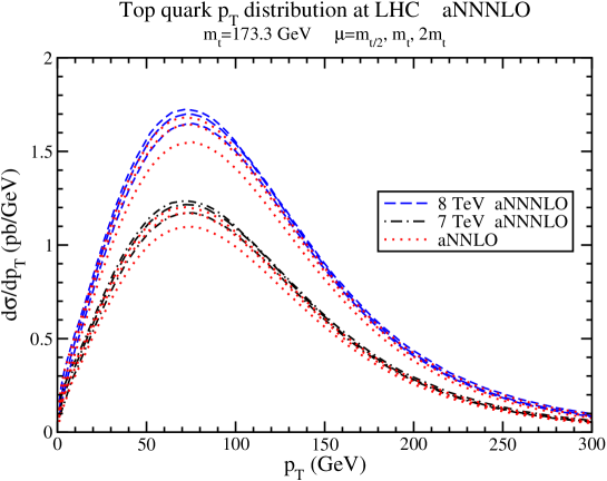
Figure 1: The aNNNLO top-quark $p_{T}$ distributions in $t{\bar{t}}$ production at the LHC with $\sqrt{S}=7$ and 8 TeV.

In Fig. 1 we show the aNNNLO top-quark $p_{T}$ distributions at 7 and 8 TeV LHC energy for $p_{T}$ values up to 300 GeV. For comparison we also show the aNNLO results at each energy. The central lines are with scale $\mu=m_{t}$, and the other lines display the upper and lower values from scale variation over the interval $m_{t}/2\leq\mu\leq 2m_{t}$ for each energy. The uncertainty from scale variation at aNNNLO is smaller than at aNNLO, a fact which is consistent with the results for the total cross section in [13].

Figure 2: The aNNNLO top-quark $p_{T}$ distributions in $t{\bar{t}}$ production at the LHC with $\sqrt{S}=13$ and 14 TeV.

In Fig. 2 we show the aNNNLO top-quark $p_{T}$ distributions at 13 and 14 TeV LHC energy, also for $p_{T}$ values up to 300 GeV. Again, for comparison, we also display the aNNLO curves for each energy. The scale variation is again smaller at aNNNLO than at lower orders.

Figure 3: The aNNNLO top-quark $p_{T}$ distributions at high $p_{T}$ in $t{\bar{t}}$ production at the LHC with $\sqrt{S}=7$, 8, 13, and 14 TeV. The inset plot shows the $K$ factors.

Figure 3 displays the aNNNLO top-quark $p_{T}$ distributions at high $p_{T}$ at LHC energies in a logarithmic plot over a larger range of transverse momenta, 300 GeV $\leq p_{T}\leq 1000$ GeV. The distributions span 4 to 5 orders of magnitude over the $p_{T}$ range shown in the figures. The inset plot displays the $K$-factors, i.e. the ratios of the aNNNLO $p_{T}$ distribution to the NLO [16, 17] result, for each energy, all with the same choice of pdf. We observe that the $K$-factors increase with increasing $p_{T}$ as would be expected since we get closer to partonic threshold.

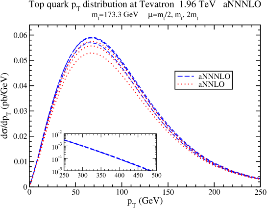
Figure 4: The aNNNLO top-quark $p_{T}$ distributions in $t{\bar{t}}$ production at the Tevatron with $\sqrt{S}=1.96$ TeV.

Figure 4 displays the aNNNLO top-quark $p_{T}$ distributions (and also the aNNLO results) at the Tevatron with 1.96 TeV energy. Again, the uncertainty from scale variation at aNNNLO is smaller than in previous calculations. The inset plot displays the high-$p_{T}$ region in a logarithmic scale up to a $p_{T}$ of 500 GeV.

As a numerical consistency check, we note that the aNNNLO cross sections found by integrating over the $p_{T}$ distributions in Figs. 1-4 agree with the results in [13].

4 Top-quark rapidity distributions

We continue with the aNNNLO top-quark rapidity distributions in $t{\bar{t}}$ production at the LHC and the Tevatron.

Figure 5: The aNNNLO top-quark rapidity distributions in $t{\bar{t}}$ production at the LHC with $\sqrt{S}=7$ and 8 TeV.

In Fig. 5 we show the aNNNLO top-quark rapidity distributions at 7 and 8 TeV LHC energy. We also show the aNNLO results at each energy. The central lines are with $\mu=m_{t}$, and the other lines display the upper and lower values from scale variation over the interval $m_{t}/2\leq\mu\leq 2m_{t}$ for each energy. The uncertainty from scale variation at aNNNLO is smaller than at aNNLO, a fact which is consistent with the results for the total cross section in [13] as well as the observations in the previous section.

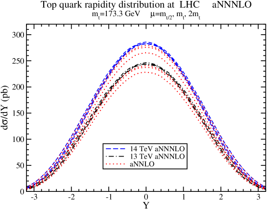
Figure 6: The aNNNLO top-quark rapidity distributions in $t{\bar{t}}$ production at the LHC with $\sqrt{S}=13$ and 14 TeV.

In Fig. 6 we show the aNNNLO (and also the aNNLO) top-quark rapidity distributions at 13 and 14 TeV LHC energy. Again, the scale variation at aNNNLO is smaller than that at aNNLO.

Figure 7: The aNNNLO top-quark rapidity distributions in $t{\bar{t}}$ production at the LHC with $\sqrt{S}=7$, 8, 13, and 14 TeV. The inset plot shows the $K$ factors.

Figure 7 displays the aNNNLO top-quark rapidity distributions at LHC energies in a logarithmic plot over a larger range of rapidities. The inset plot displays the $K$-factors, i.e. the ratios of the aNNNLO rapidity distribution to the NLO [16, 17] result, for each energy, all with the same choice of pdf. The $K$-factors are larger at the edges of the rapidity distribution, i.e. at large absolute value of the rapidity, as expected.

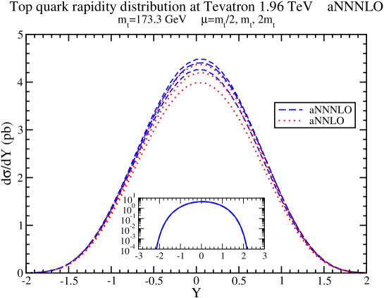
Figure 8: The aNNNLO top-quark rapidity distributions in $t{\bar{t}}$ production at the Tevatron with $\sqrt{S}=1.96$ TeV.

Figure 8 displays the aNNNLO top-quark rapidity distributions at the Tevatron at 1.96 TeV energy and, for comparison, also the aNNLO results. Again, the scale variation at aNNNLO is smaller than in previous calculations. The inset plot displays a wider rapidity region in a logarithmic scale.

As before, as a numerical consistency check, we note that the aNNNLO cross sections found by integrating over the rapidity distributions in Figs. 5-8 agree with the results in [13].

5 Conclusions

The aNNNLO top-quark transverse momentum and rapidity distributions have been calculated in $t{\bar{t}}$ production at the LHC at 7, 8, 13, and 14 TeV energies, and at the Tevatron at 1.96 TeV energy. The distributions enhance previous results but they reduce the theoretical uncertainty. The enhancement is particularly large at very high $p_{T}$ for the transverse momentum distributions and at large absolute value of the rapidity for the rapidity distributions.

References

- [1] CDF Coll., Phys. Rev. Lett. 87, 102001 (2001).
- [2] D0 Coll., Phys. Lett. B 693, 515 (2010) [arXiv:1001.1900 [hep-ex]]; Phys. Rev. D 90, 092006 (2014) [arXiv:1401.5785 [hep-ex]].
- [3] ATLAS Coll., Phys. Rev. D 90, 072004 (2014) [arXiv:1407.0371 [hep-ex]]; ATLAS-CONF-2013-099.
- [4] CMS Coll., Eur. Phys. J. C 73, 2339 (2013) [arXiv:1211.2220 [hep-ex]]; CMS-PAS-TOP-12-028.
- [5] N. Kidonakis, Phys. Rev. D 82, 114030 (2010) [arXiv:1009.4935 [hep-ph]].
- [6] N. Kidonakis, Phys. Rev. D 84, 011504(R) (2011) [arXiv:1105.5167 [hep-ph]].
- [7] N. Kidonakis, in Proceedings of HQ2013 Summer School, DESY-PROC-2013-03, p.139 [arXiv:1311.0283 [hep-ph]].
- [8] N. Kidonakis and B.D. Pecjak, Eur. Phys. J. C 72, 2084 (2012) [arXiv:1108.6063 [hep-ph]].
-
[9]
A. Ferroglia, A. Jung, and M. Schulze, in Snowmass 2013,
http://www.snowmass2013.org/tiki-download-file.php?fileId=45 - [10] Top quark working group of Snowmass 2013, arXiv:1311.2028 [hep-ph].
- [11] S. Jabeen, Int. J. Mod. Phys. A 28, 1330038 (2013).
- [12] C.E. Gerber and C. Vellidis, arXiv:1409.5038 [hep-ex].
- [13] N. Kidonakis, Phys. Rev. D 90, 014006 (2014) [arXiv:1405.7046 [hep-ph]].
- [14] N. Kidonakis, Phys. Rev. D 73, 034001 (2006) [hep-ph/0509079].
- [15] A.D. Martin, W.J. Stirling, R.S. Thorne, and G. Watt, Eur. Phys. J. C 63, 189 (2009) [arXiv:0901.0002 [hep-ph]].
- [16] W. Beenakker, H. Kuijf, W.L. van Neerven, and J. Smith, Phys. Rev. D 40, 54 (1989).
- [17] W. Beenakker, W.L. van Neerven, R. Meng, G.A. Schuler, and J. Smith, Nucl. Phys. B 351, 507 (1991).