Hierarchical probabilistic inference of cosmic shear

Abstract

Point estimators for the shearing of galaxy images induced by gravitational lensing involve a complex inverse problem in the presence of noise, pixelization, and model uncertainties. We present a probabilistic forward modeling approach to gravitational lensing inference that has the potential to mitigate the biased inferences in most common point estimators and is practical for upcoming lensing surveys. The first part of our statistical framework requires specification of a likelihood function for the pixel data in an imaging survey given parameterized models for the galaxies in the images. We derive the lensing shear posterior by marginalizing over all intrinsic galaxy properties that contribute to the pixel data (i.e., not limited to galaxy ellipticities) and learn the distributions for the intrinsic galaxy properties via hierarchical inference with a suitably flexible conditional probabilitiy distribution specification. We use importance sampling to separate the modeling of small imaging areas from the global shear inference, thereby rendering our algorithm computationally tractable for large surveys. With simple numerical examples we demonstrate the improvements in accuracy from our importance sampling approach, as well as the significance of the conditional distribution specification for the intrinsic galaxy properties when the data are generated from an unknown number of distinct galaxy populations with different morphological characteristics.

1. Introduction

All observations to date are consistent with a cosmological model in which mass is clustered on spatial scales ranging from galaxy sizes of order a kiloparsec to hundreds of megaparsecs, corresponding to angular scales on the sky of tens of arcseconds to several degrees. The cosmological mass distribution acts as a gravitational lens for all luminous sources, which imparts inhomogeneous image distortions because the mass distribution is clustered. In principle, the coherent lensing distortions of luminous sources can be used to reconstruct the 3D cosmological mass distribution over most of the observable volume of the universe. However, except near the most dense and rare mass peaks, the gravitational lensing shearing of galaxy images is a percent-level effect perturbing unknown at order unity intrinsic galaxy shapes. The ‘cosmic shear’ of galaxies therefore can only be detected through statistical correlations of large numbers of galaxy images.

Recently, cosmic shear has been used to place competitive constraints on cosmological model parameters (Jee et al., 2013; Kilbinger et al., 2013; Heymans et al., 2013; MacCrann et al., 2014; Kitching et al., 2014). All analyses of which we are aware use point estimators for the 2D ellipticities of galaxies in a catalog to infer cosmic shear effects. From the estimated galaxy ellipticity components one can compute a two-point angular correlation function that is related to the mass clustering power spectrum in the standard cosmological framework.

There are several drawbacks to existing cosmic shear inference methods that may severely limit the amount of information that can be extracted about the 3D cosmological mass distribution and underlying cosmological model, for a given set of observations (LSST Dark Energy Science Collaboration, 2012). Bernstein & Armstrong (2014) (BA14) give a review of the primary challenges in existing methods including low signal-to-noise, large instrumental and observational systematics, finite pixel sampling, uncertainty in the morphologies of galaxies prior to lensing distortions, and biased ellipticity estimators in the presence of pixel noise.

As in BA14 and also Sheldon (2014), Miller et al. (2007, 2013) we consider a probabilistic model for cosmic shear inference that can in principle avoid many of the weaknesses in existing methods. Unlike in BA14 we initially set aside issues of computational feasibility and aim to specify a statistical framework that is a complete description of the data (i.e., including all physical parameters that are needed to completely describe the measured pixel values in a photometric survey). While we see value in simply writing down the complete statistical framework for cosmic shear we were also able to identify statistical sampling and computational algorithms that are likely to make our framework practical for upcoming surveys. We demonstrated a simple implementation of our framework in the GREAT3 community cosmic shear measurement challenge (Mandelbaum et al., 2013) and further demonstrate the computational performance of our framework in subsequent papers (Bard et al., in prep.; Meyers et al., in prep.).

Most of the parameters that are needed to describe the pixel data are uninteresting for cosmology and can be marginalized out; this is an advantage of probabilistic modeling. If we can infer probability distribution functions (PDFs) for the nuisance parameters and marginalize—instead of either asserting distributions or else fixing the nuisance parameters to heuristically chosen or maximum-likelihood values—we expect to obtain better (more accurate and also more conservative) inferences about the cosmological parameters. Adopting this probabilistic approach moves us (relative to other methods) along the bias–variance trade-off towards less biased inferences. Of course, in the context of fully probabilistic inference, without point estimators, there isn’t as clear a definition of “bias” and it may be difficult to put the long literature on weak-lensing biases into context here. However, we expect many of the known biases in point estimators to be ameliorated when we permit the freedom to infer and marginalize out nuisances. In detail, as we give more freedom to the model (more flexibility in the nuisance-parameter space), we will move to even less biased (though also probably less precise) inferences, possibly at large computational cost.

Explicit specification or inference of the distributions of all model parameters not only has the potential to reduce biases in the shear inference but also is the only way to guarantee an optimal measurement (in the sense that no other accurate inference method could yield tighter marginal posterior distributions on the cosmological model parameters). Most past cosmic shear analyses have not specified the distributions of galaxy intrinsic properties and observing conditions (e.g., the PSF) that are assumed in their cosmological inferences. But, because intrinsic galaxy properties and observing conditions do describe important features of the data, all cosmic shear analyses must have (at least implicitly) marginalized over some distributions in these parameters. Implicit marginalization over un-specified priors cannot yield an optimal measurement. Said another way, without explicit marginalization of model parameters it is not possible to saturate the Cramér-Rao bound (e.g. Kendall, M. G. & Stuart, A., 1969). In particular, analyses in which measured ellipticities of galaxies are averaged together over sky patches (or something equivalent) have made an implicit (and strong) assumption about the distribution of intrinsic shapes; this assumption (since unexamined) is likely to be sub-optimal at best.

Once a complete statistical model is specified, there are three key practical challenges for probabilistic shear inference,

1. Specification of an interim model describing galaxy morphologies, flux profiles, and spectral energy distributions. Galaxy features are complex and multi-faceted because of the evolution of galaxy properties with cosmic time, galaxy mergers, and varying environments. The observable features of galaxies are further complicated by object blending that may mimic intrinsic features of the galaxy population (Dawson et al., 2014). We require a parametric model for galaxies and a likelihood function that can describe all such variations in galaxy images over the model parameter ranges that are important for describing the data. With an incomplete galaxy parametric model and without propagating all the information about the model in the likelihood function, it is well known that ‘model fitting biases’ can be catastrophic for cosmic shear (Voigt & Bridle, 2010; Melchior et al., 2010; Bernstein, 2010; Kacprzak et al., 2014).

2. Specification of the probability distribution for the galaxy model parameters to be marginalized in the shear inference. While the accurate specification of models for galaxy images may sound challenging to the discerning reader, the specification of the joint distribution of intrinsic galaxy properties is perhaps even more daunting. A primary aim of this paper is to describe and demonstrate how a hierarchical model can allow meaningful inference of the properties of the galaxy distribution simultaneously with the shear. Without hierarchical inference (i.e., inferring the distributions of nuisance parameters) we are susceptible to an ‘overconfidence problem’ wherein asserting a prior that is too simple can yield inferences that appear more precise than warranted.

3. Monte Carlo sampling of model parameters from the joint posterior distribution given multi-epoch imaging of a large galaxy survey. Because both the shear and the PSF vary in correlated ways over any given image, the inferences for different galaxies are statistically dependent. In a straightforward probabilistic inference we would need to fit model parameters simultaneously to all galaxy images, which is a formidable computational challenge. Instead we sample model parameters for each galaxy independently and perform a subsequent joint inference using importance sampling given interim posterior samples for each galaxy image.

In Section 2 we outline our framework for the complete cosmic shear inference problem. In subsection 2.1 we enumerate the components the framework and in subsection 2.2 we outline the key algorithms we use for Monte Carlo sampling of model parameters to render our framework computationally feasible. In Section 3 we focus on implementation details for just the inference of intrinsic galaxy properties, leaving similar details for the PSF and lensing mass inferences to future work. We describe our model for the distribution of intrinsic galaxy properties in subsection 3.1 and give numerical examples of shear and ellipticity inferences in subsection 3.2. In Section 4 we discuss how to expand the inferences demonstrated for the intrinsic ellipticity distribution to the PSF and lensing mass models and summarize our conclusions. We refer the reader to Bard et al. (in prep.) for further discussion of parameterized models for galaxy images and the integration of such models in our sampling framework.

2. Part 1: Description of the statistical framework

2.1. Three conditionally independent branches

We begin this section by enumerating the variables and dependencies of a complete statistical framework for shear inference. In subsequent sections we demonstrate the inference of a subset of the variables in our framework with numerical models. We defer a more detailed examination of some aspects of the statistical framework to later publications. But we believe it is useful at this stage to list all contributions to the cosmic shear inference problem given the considerable literature on the subject that has not yet converged on a unified statistical picture.

Table 1Sampling parameters for the full statistical model. The central line separates sampled from conditional parameters.

Parameter	Description
$\bm{\theta}$	Cosmological parameters
$\psi_{s}$	2D lens potential (given source photo-$z$ bin $s$)
${\Pi}_{i}$	PSF in epoch $i$
$\Omega_{i}$	Observing conditions in epoch $i$
$\{\omega_{n}\}$	Galaxy model parameters; $n=1,\dots,n_{\rm gal}$
$\{\alpha_{n}\}$	Parameters for the distribution of $\{\omega_{n}\}$
$\{\xi_{n}\}$	Scaling parameters for $\{\omega_{n}\}$
$m,\tau$	Hyperprior parameters for $\{\xi_{n}\}$
$\mathcal{A}$	Hyperparameter for $\{\alpha_{n}\}$ classifications
$\{{\mathbf{d}}_{n}\}$	Pixel data for galaxies $n=1,\dots,n_{\rm gal}$
$G_{0}|a_{\eta}$	Prior specification for $\{\alpha_{n}\}$
$s$	Source sample (e.g., photo-$z$ bin)
$W$	Survey window function
${\mathbf{d}}_{{\rm anc},i}$	Ancillary data for PSF in epoch $i$
$p$	Prior params. for observing conditions
$a$	Prior params. for $\mathcal{A}$
$\sigma_{\rm pix}$	Pixel noise r.m.s.
$I$	Model selection assumptions

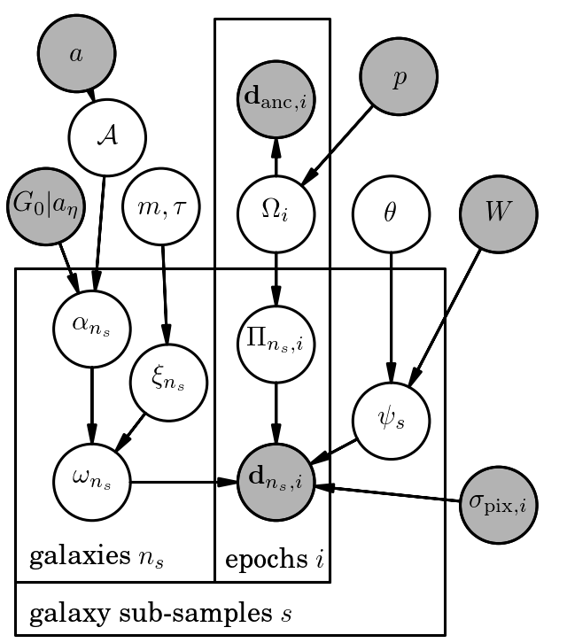
Figure 1.— Probabilistic graphical model for our complete framework for shear inference. Arrows indicate statistical dependencies. Grey shading indicates quantities that are not sampled. For the lens potential $\psi$ we include only the dependencies in the marginal distributions after integrating out the line-of-sight distribution uncertainties contributing to the lens potential.

2.1.1 Lensing mass distribution

We start by specifying the parameters $\bm{\theta}$ of the cosmological model, sampled from a prior distribution ${\rm Pr}(\bm{\theta})$ given all past cosmological experiments. Although not explicitly implemented in this paper, we expect $\bm{\theta}$ to include parameters such as the mean mass density $\Omega_{m}$ and the r.m.s. of mass density fluctuations $\sigma_{8}$ that primarily determine the amplitude of the cosmic shear correlation function.

From these parameters, we can predict the 3D cosmological mass distribution, described by the 3D gravitational lensing potential $\Psi$. Assuming, for example, Gaussian initial conditions $\Psi^{\rm initial}$ for the 3D mass density in the early universe and gravitational evolution according to General Relativity, the probability distribution for the late-time 3D mass density $\Psi$ responsible for gravitational lensing of galaxies depends only on the cosmological parameters and the initial conditions, ${\rm Pr}(\Psi|\bm{\theta},\Psi^{\rm initial})$. We discuss possibilities for inferring constraints on $\Psi$ in subsubsection 2.2.1 but otherwise confine our analyses to the inference of gravitational lensing quantities after projecting the 3D gravitational potential $\Psi$ over the line-of-sight distribution of lenses in a survey.

We define the 2D lensing potential that describes the shearing (and magnification) of any sample of galaxies in a survey by the following integral of the 3D potential $\Psi$ (see, e.g., equation 6.14 of Bartelmann & Schneider, 2001) (also section 3.2 of Narayan & Bartelmann, 1996),

$$\bar{\psi}_{s}(\mathbf{x})\equiv W(\mathbf{x})\int da\,\Psi(\mathbf{x},a)K(a;A_{s}),$$ ((1))

where $a$ is the cosmological scale factor in the Freidmann equation, $\mathbf{x}$ are the coordinates in the plane of the sky, $W(\mathbf{x})$ is the angular window function of the survey, the subscript $s$ denotes a particular sample of ‘source’ galaxies that are lensed by the foreground potential $\Psi$, and $K$ is the lensing kernel including the lensing efficiency based on the distances between observer, lens, and sources, and the integral over the source distribution with parameters $A_{s}$ (see equation 6.19 of Bartelmann & Schneider, 2001).

The parameters $A_{s}$ can include the uncertainties in the survey redshift distribution (e.g., from photometric redshift errors, see Loh & Spillar, 1986; Connolly et al., 1995; Huterer et al., 2006) as well as other astrophysical systematics that are redshift-dependent (such as intrinsic alignments of galaxies, see Catelan et al., 2001; Bridle & King, 2007). Marginalizing the nuisance parameters in the line-of-sight projection, the 2D lensing potential $\psi$ given the cosmology and survey sample is distributed according to,

$${\rm Pr}(\psi_{s}|\theta,s,W)\propto\int d\Psi\,{\rm Pr}(\Psi|\bm{\theta})\\ \times\int dA_{s}\,{\rm Pr}(\psi_{s}|\Psi,A_{s},W){\rm Pr}(A_{s}|\bm{\theta},s,W).$$ ((2))

For a deterministic cosmological model (as emphasized in Jasche & Wandelt, 2013), ${\rm Pr}(\psi|\Psi,A,W)\propto\delta_{\rm D}\left(\psi-\bar{\psi}(\Psi,A,W)\right)$, where $\delta_{\rm D}$ is the Dirac delta function.

2.1.2 Point-spread functions

To connect the lens potential to the observable properties of galaxy images, we must also specify the distribution of the point-spread function (PSF) realizations specific to the (time-variable) observing conditions at epoch $i$ given parameters $\Omega_{i}$ such as the seeing, optics alignments, and detector response, ${\rm Pr}({\Pi}_{i}|\Omega_{i})$. For given $\Omega$, the PSF ${\Pi}(\mathbf{H}_{n};\Omega)$ can be computed at the focal plane position $\mathbf{H}_{n}$ for any galaxy $n$. The observing conditions $\Omega_{i}$ in an observation epoch $i$ will not be known perfectly but will be constrained by ancillary data ${\mathbf{d}}_{\rm anc}$ and a distribution ${\rm Pr}(\Omega_{i}|p)$ conditioned on time-independent PSF model parameters $p$ (e.g., the allowed distributions of optics distortions or atmospheric turbulence power spectra). The complete model for the PSF at all field positions $\mathbf{H}_{n}$ in observation epoch $i$ is not separable for different field positions after marginalizing over the observing conditions,

$${\rm Pr}(\left\{{\Pi}_{n,i}\right\}_{n=1}^{n_{\rm gal}}|\left\{\mathbf{H}_{n}\right\}_{n=1}^{n_{\rm gal}},{\mathbf{d}}_{{\rm anc},i},p)=\\ \int d\Omega_{i}\,\left[\prod_{n=1}^{n_{\rm gal}}{\rm Pr}({\Pi}_{n,i}|\mathbf{H}_{n},\Omega_{i})\right]\\ \times{\rm Pr}({\mathbf{d}}_{{\rm anc},i}|\Omega_{i}){\rm Pr}(\Omega_{i}|p).$$ ((3))

where ${\rm Pr}({\mathbf{d}}_{{\rm anc},i}|\Omega_{i})$ is the likelihood of the ancillary data given the specific observing conditions in epoch $i$. We will refer to Equation (3) as our ‘probabilistic PSF model’.

Note however, that we infer a distinct PSF realization ${\Pi}_{n,i}$ for each galaxy $n$ in each observation epoch $i$, which are related across galaxies in a given epoch by the common observing conditions $\Omega_{i}$. The PSFs in different epochs are further related by another level of hierarchy with a common PSF model with parameters $p$. So, we can also directly marginalize the likelihood over the PSF realizations,

$${\rm Pr}({\mathbf{d}}|\{\omega_{n}\},\psi,p)=\prod_{n=1}^{n_{\rm gal}}\prod_{i=1}^{n_{\rm epoch}}\int d\Omega_{i}\,{\rm Pr}(\Omega_{i}|p)$$

$$\times\int d{\Pi}_{n,i}\,{\rm Pr}\left({\Pi}_{n,i}|\Omega_{i}\right){\rm Pr}\left({\mathbf{d}}_{n,i}|\omega_{n},\psi,{\Pi}_{n,i}\right)$$

$$=\prod_{i=1}^{n_{\rm epoch}}\int d\Omega_{i}\,{\rm Pr}(\Omega_{i}|p)\left[\prod_{n=1}^{n_{\rm gal}}{\rm Pr}\left({\mathbf{d}}_{n,i}|\omega_{n},\psi,\Omega_{i}\right)\right]$$ ((4))

$$=\prod_{i=1}^{n_{\rm epoch}}{\rm Pr}\left({\mathbf{d}}_{i}|\{\omega_{n}\},\psi,p\right)$$ ((5))

$$\neq\prod_{n=1}^{n_{\rm gal}}{\rm Pr}\left({\mathbf{d}}_{n}|\omega_{n},\psi,p\right)$$ ((6))

Marginalizing the PSF realizations ${\Pi}_{n,i}$ over all galaxies $n$ in a given epoch $i$ still yields a likelihood function that is separable for separate objects $n$ Equation (4), conditioned on the observing conditions $\Omega_{i}$. This shows that more information about the observing conditions $\Omega_{i}$ leads to smaller statistical correlations among the marginal likelihoods for different galaxies independent from the actual PSF realizations. Under our framework therefore, it is the parameters of the distribution from which PSF realizations are drawn that are most important to constrain rather than estimation and interpolation of PSF realizations at different image plane locations.

2.1.3 Intrinsic source properties

Finally, the intrinsic properties $\omega_{n}$ of a model for galaxy $n$ (e.g., ellipticity, size, brightness) are described by the distribution

$${\rm Pr}(\omega_{n}|\alpha,I),$$ ((7))

where $\alpha$ are parameters in the distribution of the intrinsic galaxy properties and $I$ denotes galaxy modeling assumptions (such as the form of the galaxy morphology parameterization). For example, $\alpha$ could describe the width of the intrinsic (i.e., unlensed) ellipticity distribution of a given galaxy population. And in Bard et al. (in prep.), the model assumptions $I$ include modeling all galaxies as elliptical Sérsic profiles. It will be important to keep $I$ explicit as we consider possible model-fitting biases in our framework (Voigt & Bridle, 2010; Kacprzak et al., 2014; Bard et al., in prep.).

2.2. Sampling methods to divide and conquer

2.2.1 Interim sampling of model parameters for individual sources

The pixel data ${\mathbf{d}}_{n}$ in the vicinity of a galaxy $n$ enters our framework only through the likelihood function

$${\rm Pr}({\mathbf{d}}_{n}|\omega_{n},\psi,{\Pi}).$$ ((8))

We can reasonably assume uncorrelated noise in the common case that sky noise (i.e., Poisson noise from sky background) dominates the noise in the pixel values, giving a likelihood function,

$$\ln{\rm Pr}({\mathbf{d}}_{n})=-\frac{1}{2}\sum_{i=1}^{n_{\rm epochs}}\frac{\left({\mathbf{d}}_{n,i}-\bar{{\mathbf{d}}}\left(\omega_{n},\psi,{\Pi}_{i}\right)\right)^{2}}{\sigma_{{\rm pix},n,i}^{2}}+{\rm const.},$$ ((9))

where $\bar{{\mathbf{d}}}$ is the model prediction for the pixel values, $i$ indexes multiple observation epochs, and $\sigma_{{\rm pix},n,i}$ is the noise r.m.s. per pixel for object $n$ in epoch $i$. Note the model prediction in the likelihood includes the PSF ${\Pi}_{i}$ for each observation $i$ of a given galaxy $n$. This makes the model predictions potentially expensive to compute unless the convolution of the PSF with the galaxy model can be done efficiently. We will return to this issue in Appendix A and Bard et al. (in prep.). We discuss the alternative proposed by BA14 of using moments of the galaxy intensity profiles in place of pixel values in Appendix F.

In Equation (8) we have assumed that the likelihood function for all sources in an image can be factored into a product of likelihoods for distinct sources. This will not be true in when the pixel noise is correlated for sources that are adjacent on the sky (e.g., when unresolved flux contaminates the pixels of neighboring sources).

The model prediction $\bar{{\mathbf{d}}}$ for the pixel values of a galaxy image depends on the cosmological mass density $\psi$ through the action of gravitational lensing on the galaxy morphology and flux (in any given bandpass as lensing is achromatic). For simple elliptical models of galaxies, the ellipticity parameter in $\omega_{n}$ is degenerate with the reduced shear $g\equiv\gamma/(1-\kappa)$. However, the statistical distribution of all elements of $\omega$ should be isotropic across different galaxies in the sky (although this is not true for small fields, e.g., around a cluster), while the ellipticities of lensed galaxy images are not. We therefore maintain a conceptual distinction between $\omega_{n}$ and $\psi$ in the model for pixel values of a galaxy image $\bar{{\mathbf{d}}}$ even though this distinction is not computationally meaningful for the simplest models of galaxy images. See also the discussion following Equation (15) below.

The first step in our computational algorithm is to draw ‘interim samples’ of $(\omega_{n},\psi,{\Pi}_{n,i})$ via Markov Chain Monte Carlo (MCMC) from the likelihood in Equation (9) for a single source (or region of sky) identified in all available exposures of a survey. The method of source identification for selecting the pixel values ${\mathbf{d}}_{n}$ in Equation (9) is not important as long as our model predictions for the observed pixels allow for observationally truncated source profiles or multiple overlapping sources (as will be needed for blended objects). Allowing for such selection effects may also admit interim sampling of the combined pixel data from different instruments or surveys.

Lensing mass inference

The intrinsic galaxy properties $\omega_{n}$ and the PSF ${\Pi}_{n,i}$ can be interim sampled with distinct parameters for each object. We might consider interim sampling uncorrelated shears and magnifications for every object, but in most cases the shear and the intrinsic ellipticity are strongly degenerate for isolated objects (the exception being resolved galaxy images with multiple morphological components that have different responses to the action of an applied shear). To infer a shear or lens potential that varies over the sky, we then need to specify the model correlations between shears at different sky locations and redshifts. This is distinct from conventional algorithms that involve cross-correlating galaxy ellipticity estimators at different sky locations. We instead seek a generative model for the shear correlations.

We can infer variable shear models without a cosmological prediction of the mass density (which can be computationally expensive) by specifying an interim prior for the lens potential $\psi_{s}$ for a given source distribution. The only requirement is that the mathematical specification of the interim prior for $\psi_{s}$ allows for spatial correlations that encapsulate the possible cosmological interpretations.

In practice, we first sample galaxy model parameters without a correction for the applied shear and magnification. Given the galaxy model parameters, we can then reinterpret the parameters under an assumed lens potential model because we know how lensing affects the model for the galaxy light profile. We therefore ignore the lensing parameters in the first step of our inference, including a model for lensing shears and magnifications only when combining inferences from distinct sources as we describe next.

2.2.2 Hierarchical inference via importance sampling

It is possible to infer model constraints independently for each galaxy and then combine these independent inferences in a hierarchical framework using the technique of ‘importance sampling’ (e.g. Geweke, 1989; Wraith et al., 2009; Hogg et al., 2010).

Our goal with the importance sampling algorithm is to evaluate the likelihood marginalized over individual galaxy intrinsic properties and PSF realizations,

$${\rm Pr}({\mathbf{d}}|\alpha,\Omega,\psi)\propto\prod_{n=1}^{n_{\rm gal}}\int d\omega_{n}\,{\rm Pr}(\omega_{n}|\alpha)\\ \times\prod_{i=1}^{n_{\rm epoch}}\int d{\Pi}_{n,i}\,{\rm Pr}({\Pi}_{n,i}|\Omega_{i})\\ \times{\rm Pr}({\mathbf{d}}_{n,i}|\omega_{n},\psi,{\Pi}_{n,i}),$$ ((10))

where

$${\mathbf{d}}\equiv\left\{\left\{{\mathbf{d}}_{n,i}\right\}_{i=1}^{n_{\rm epoch}}\right\}_{n=1}^{n_{\rm gal}},$$ ((11))

and $\Omega\equiv\left\{\Omega\right\}_{i=1}^{n_{\rm epoch}}$. Using the identity,

$$\int dx\,p(x)f(x)=\int dx\,p(x)g(x)\frac{f(x)}{g(x)},$$ ((12))

for arbitrary probability distributions $p(x),f(x)$ and assuming $g(x)$ has nonzero probability mass over the domain where $f(x)$ is nonzero, we can factor Equation (10) as,

$${\rm Pr}({\mathbf{d}}|\alpha,\Omega,\psi)\propto\prod_{n=1}^{n_{\rm gal}}\prod_{i=1}^{n_{\rm epoch}}\int d\omega_{n}\int d{\Pi}_{n,i}\,\\ \times\frac{{\rm Pr}(\omega_{n}|\alpha)}{{\rm Pr}(\omega_{n}|I_{0})}\frac{{\rm Pr}({\Pi}_{n,i}|\Omega_{i})}{{\rm Pr}({\Pi}_{n,i}|I_{0})}\\ \times{\rm Pr}({\mathbf{d}}_{n,i}|\omega_{n},\psi,{\Pi}_{n,i}){\rm Pr}(\omega_{n}|I_{0}){\rm Pr}({\Pi}_{n,i}|I_{0}).$$ ((13))

The final line of Equation (13) defines the ‘interim posterior’ from which we draw samples when we analyze each galaxy independently (following Hogg et al., 2010). We refer to ${\rm Pr}(\omega_{n}|I_{0})$ and ${\rm Pr}({\Pi}_{i}|I_{0})$ as ‘interim priors’. The interim priors can be chosen to make computations convenient. We have found flat or broad Gaussian distributions to be sufficient interim prior specifications.

We use the following algorithm to combine samples from the interim posteriors for each galaxy into a hierarchical inference of the global marginal posterior. For each object $n$ we generate $K$ samples $\left[\omega_{nk},\left\{{\Pi}_{nik}\right\}_{i=1}^{n_{\rm epoch}}\right]$, sampled from the interim posterior given pixel data for galaxy $n$ in all epochs,

$${\rm Pr}\left(\omega_{n},{\Pi}_{n}|{\mathbf{d}}_{n}\right)=\frac{1}{Z_{n}}\\ \times{\rm Pr}\left({\mathbf{d}}_{n}|\omega_{n},{\Pi}_{n}\right){\rm Pr}\left(\omega_{n}|I_{0}\right){\rm Pr}\left({\Pi}_{n}|I_{0}\right),$$ ((14))

where $Z_{n}$ is a normalization that we never need to compute, and $I_{0}$ denotes the set of assumptions encoded into the interim priors. Once we have this $K$-element interim sampling for every galaxy $n$ we can build importance-sampling approximations to various other marginalized likelihoods. Specifically, for the integral in Equation (13), the marginalized likelihood can be approximated by

$${\rm Pr}({\mathbf{d}}_{n}|\alpha,\Omega,\psi) \approx\frac{Z_{n}}{K}\sum_{k}\frac{{\rm Pr}(\omega_{nk}|\alpha,\psi)}{{\rm Pr}(\omega_{nk}|I_{0})}\frac{{\rm Pr}({\Pi}_{nk}|\Omega)}{{\rm Pr}({\Pi}_{nk}|I_{0})},$$ ((15))

$${\rm Pr}({\mathbf{d}}|\alpha,\Omega,\psi) =\prod_{n=1}^{n_{\rm gal}}{\rm Pr}({\mathbf{d}}_{n}|\alpha,\Omega,\psi).$$ ((16))

What we have achieved with Equation (15) is the ability to fit galaxy models and PSFs to individual galaxies (via MCMC) and then to combine the fit information from each galaxy into inferences on the distributions of intrinsic galaxy properties $\alpha$ and PSF parameters $p$. Equation (15) is fast to compute once the $K$ samples for each galaxy are generated. For the final shear inference we will marginalize the parameters $\alpha$, but with Equation (15) we have already addressed the primary computational bottleneck in modeling images of large numbers of sources in a field.

Although not part of the preceding derivation, we inserted the lensing potential $\psi$ into the list of conditional dependencies in the numerator of Equation (15). This is because given interim posterior samples of galaxy model parameters, we can always reinterpret those model parameters under a different assumption for the shear for any model where we know how to calculate the action of shear on the model galaxy.

To evaluate Equation (15) we need $K$ independent samples from the interim posteriors for each galaxy. While this can be slow to generate via MCMC when $K$ is required to be large, we have found in simple tests that even $K=1$ may be sufficient when assuming a constant shear over a given area of the sky (Meyers et al., in prep.). We use $K=10$ in the numerical examples in Section 3.

Importance sampling the lens potential

Given interim samples of the lens potential $\psi_{s}$ we can then infer cosmological parameter constraints from the sampled lens potentials for all galaxy samples in all fields using importance sampling as in Equation (15), but with a new conditional PDF that includes the dependence of the lens potential cosmological parameters $\bm{\theta}$ and the cosmological initial conditions $\Psi^{\rm initial}$,

$${\rm Pr}({\mathbf{d}}_{n}|\Psi^{\rm initial},\theta,W)\propto\frac{1}{N}\sum_{k=1}^{N}\frac{\prod_{s}{\rm Pr}(\hat{\psi}_{s,k}|\Psi^{\rm initial},\theta,W)}{\prod_{s}{\rm Pr}(\hat{\psi}_{s,k}|I)},$$ ((17))

where, again, we have implicitly marginalized over the line-of-sight distribution error parameters $A_{s}$ from Equation (2).

Equation (17) also helps to understand the utility in separating the galaxy population into different samples $s$. It is straightforward to derive separate inferences of $\Psi^{\rm initial}$ and $\bm{\theta}$ for different sub-samples $s$ of the galaxies to test for consistency with respect to unmodeled systematic errors or new physical phenomena not captured by the cosmological model for the mass density evolution. One could similarly infer different distributions of the intrinsic galaxy properties $\omega$ for different sub-samples to test for variable model fitting biases and unmodeled redshift evolution in the galaxy population. But, once we have computed the inferences of the 2D lens potential for different sub-samples $s$, the combined inference of cosmology in Equation (17) is not much more complicated than that for an undivided galaxy sample.

An algorithm as in Equation (17) could also obviate the need to compute covariances of cosmological correlation functions between tomographic redshift bins, which is estimated to be a formidable challenge for upcoming surveys (Dodelson & Schneider, 2013; Taylor et al., 2013; Morrison & Schneider, 2013)

To summarize, by placing an interim prior on $\psi$ that includes spatial correlations over the observed sky area, we stand to gain from a similar computational factorization of the analysis as that achieved with the model for the intrinsic galaxy properties. Most published cosmic shear analyses follow a reverse algorithm where the shear is estimated, turned into two-point correlation estimators and compared with a two-point correlation model. Instead, our framework must start with the two-point correlation model (for a Gaussian density field), realize the shear field, apply the realized shear to each galaxy model and then compare the pixel model with the data for each galaxy. We consider the computational separation of each of these steps to be a key benefit of the framework we present here.

Finally, one should keep in mind that the relationship between the lens potential defined over the sky and the lensing distortions of measured galaxy images are dependent on the astrometric solution for each exposure. However, we expect this to be a negligible contribution to the shear inference in most cases. Possible centroid shifts of galaxy images should instead be captured by the PSF model.

2.3. Statistical framework summary

In Sections 2.1 and 2.2 we introduced a number of parameters with nontrivial interdependencies. Here we collect all the parameters we have introduced and summarize the statistical framework by presenting the factorization of the unmarginalized joint posterior for all sampled model parameters,

$${\rm Pr}(\bm{\theta},\{\psi_{s}\},\{{\Pi}_{i},\Omega_{i}\},\{\omega_{n},\alpha_{n},\xi_{n}\},\mathcal{A},\tau,m,a_{\eta}|\{{\mathbf{d}}_{n}\},\mathcal{X})\propto\\ {\rm Pr}\left(\bm{\theta}\right)\cdot{\rm Pr}\left(\{\psi_{s}\}|W,\{s\},\bm{\theta}\right)\cdot{\rm Pr}(\mathcal{A}|a)\\ \times\prod_{n=1}^{n_{\rm gal}}{\rm Pr}(\omega_{n}|\alpha_{n},I)\cdot{\rm Pr}(\alpha_{n}|\mathcal{A},a_{\eta})\cdot{\rm Pr}(\xi_{n}|m,\tau)\\ \times\prod_{i=1}^{n_{\rm epoch}}{\rm Pr}\left({\Pi}_{n,i}|\Omega_{i},I)\cdot{\rm Pr}(\Omega_{i}|p,{\mathbf{d}}_{{\rm anc},i}\right)\\ \times{\rm Pr}\left({\mathbf{d}}_{n,i}|\omega_{n},\xi_{n},\psi_{s},{\Pi}_{n,i}\right)$$ ((18))

where in the first line we collapsed the conditional parameters into,

$$\mathcal{X}\equiv\left[{\mathbf{d}}_{\rm anc},\{s\},W,a,p,I\right].$$ ((19))

We collect the definitions of all variables in Equation (18) in Table 1 and display the statistical dependencies in Figure 1.

The final line of Equation (18) is the likelihood function for the pixel data ${\mathbf{d}}_{n,i}$ of galaxy $n$ in observation epoch $i$, which depends on the intrinsic galaxy properties $\omega_{n},\xi_{n}$, the lensing potential $\psi_{s}$ for source sample $s$ containing galaxy $n$, and the PSF ${\Pi}_{n,i}$. The preceding lines in Equation (18) describe the hierarchical PDFs for the conditional dependencies in the likelihood function, including the important factorizations across distinct galaxies and observation epochs. In subsection 4.1 we discuss how marginalization of the conditional dependencies in the likelihood couples the inference from individual galaxies and epochs as determined by the hierarchical parameters that are constant across galaxies and epochs in Equation (18) (e.g., parameters that do not have $n$ or $i$ subscripts).

Note also we assumed in Equation (18) that the errors in the line-of-sight distribution (e.g., photo-$z$ errors) are already marginalized as in Equation (2). We reserve a more thorough exploration of line-of-sight parameter modeling for future work.

3. Part 2: Implementation for inferring intrinsic galaxy properties

3.1. Model for the conditional distribution of intrinsic galaxy properties

We choose a non-parametric distribution to describe the galaxy model parameters both because we have little information to guide us on the choice of a parametric distribution and because we need a flexible distribution to minimize any biases in the model parameter inferences (as mentioned in Section 1). We therefore choose a Dirichlet Process (DP) model (e.g. Ferguson, 1973; Walker et al., 1999; Neal, 2000; Müller & Quintana, 2004; Wang & Dunson, 2011) for the distribution of intrinsic galaxy properties, with distinct parameters $\alpha_{n}$ for each galaxy $n$.

Assuming a Normal (i.e., Gaussian) distribution for the intrinsic galaxy properties $\omega$, the DP model can be represented by the following hierarchy (Neal, 2000, Eqn. 2.1),

$$\omega_{n}\sim\mathcal{N}(0,\alpha_{n}),\quad\alpha_{n}\sim G(\alpha_{n}|\mathcal{A}),\quad G\sim{\rm DP}(\mathcal{A},G_{0}),$$ ((20))

where $\mathcal{N}$ indicates the Normal distribution with mean and (co)variance parameters. We assume a Normal distribution for $\omega_{n}$ in Equation (20) both for specificity and because it is sufficient for all our numerical studies in Section 3. Equation (20) indicates that for every galaxy $n$ the properties $\omega_{n}$ of that galaxy (such as ellipticity, size, and flux) are Gaussian distributed with variance parameters $\alpha_{n}$. The subscript on $\alpha_{n}$ indicates we allow for different variances for every galaxy. Without a statistical model that relates inferences of $\alpha_{n}$ for different $n$ we would then be assuming that every galaxy in the universe is realized from a distinct generative (i.e., physical) mechanism from every other galaxy. This is of course not consistent with our understanding of cosmology and galaxy formation. Instead we introduce relationships between $\alpha_{n}$ parameters for different galaxies $n$ by means of the DP model.

Another way to think about Equation (20) is that we specify a distribution on $\omega$ that is a mixture of distributions with parameters $\alpha\sim G_{0}$ with a hyperprior on the mixing proportions given by the Dirichlet distribution.

For sampling algorithms it is useful to first marginalize the distribution $G$ in Equation (20) to get the conditional updates (eq. 2.2 of Neal, 2000),

$$\alpha_{n}|\alpha_{1},\dots,\alpha_{n-1}\sim\frac{1}{n-1+\mathcal{A}}\sum_{\ell=1}^{n-1}\delta_{\rm D}\left(\alpha_{\ell}\right)\\ +\frac{\mathcal{A}}{n-1+\mathcal{A}}G_{0}(\cdot),$$ ((21))

where $n$ indexes galaxies and $\delta_{\rm D}$ is the Dirac delta function. Given the discreteness property of the DP there is nonzero probability that draws of $\alpha_{n}$ will be repeated. Let $\alpha^{*}_{1},\dots,\alpha^{*}_{K}$ be the unique values among $\alpha_{1},\dots,\alpha_{n-1}$, and let $N_{c}$ be the number of repeats of $\alpha^{*}_{c}$ in the “latent class” $c$. Then the conditional update distribution can be equivalently written as (eq. 10 of Teh, 2010)

$$\alpha_{n}|\alpha_{1},\dots,\alpha_{n-1}\sim\frac{1}{n-1+\mathcal{A}}\\ \left(\sum_{c=1}^{K}N_{c}\delta_{\rm D}\left(\alpha^{*}_{c}\right)+\mathcal{A}G_{0}\left(\cdot\right)\right).$$ ((22))

This equation is useful because it shows the clustering properties of the DP and the meaning of the parameter $\mathcal{A}$. The value of $\alpha^{*}_{c}$ will be assigned to $\alpha_{n}$ with probability proportional to the number of times $\alpha^{*}_{c}$ has be previously drawn, $N_{c}$. Note that when $\mathcal{A}$ is large, successive values for $\alpha_{n}$ are drawn from the base distribution $G_{0}$ with high probability, generating a new $\alpha^{*}_{K}$ each time. When $\mathcal{A}$ is small, $\alpha_{n}$ is assigned to one of the previous values of $\alpha^{*}_{c}$ with high probability. We will refer to groups of galaxies $\{n\}$ that have equal values of $\alpha^{*}_{k}$ as a ‘cluster’ or ‘sub-population’, representing potential galaxy type classifications (analogous to the common ‘early-’ or ‘late-type’ classifications). Equation (21) shows that larger values of $\mathcal{A}$ will lead to more clusters or categories of galaxy types while bringing $\mathcal{A}$ to zero will force all galaxies to be assigned to the same cluster or type classification. Note that as long as the observations are exchangeable (which is true for sources in an image), the ordering of values in $\alpha$ is arbitrary.

To summarize, we are motivated to use the DP model for the following reasons,

• The DP is analogous to a mixture model when the number of mixture components is learned from the data,

• Samples for galaxy $n$ are naturally informed by those for galaxies $1,\dots,n-1$, thereby improving the sampling efficiency (for arbitrary ordering of observed galaxies),

• The DP can find unknown clusters in the galaxy parameters, teaching us about galaxy formation and different prospects for shear inference from different data subsets. For example, we show in subsubsection 3.2.2 that knowledge of a galaxy sub-population that is more round than average can improve the shear inference.

With such an algorithm to cluster the features in the galaxy population we are able to simultaneously fit different distributions for each galaxy and exploit the statistical information from a large sample of galaxies. As we will see in Section 3, the DP model (rather than a less flexible asserted prior distribution) can be an important component of our framework for improving the accuracy and precision of the shear inference.

For later Gibbs sampling we found it more helpful to consider the DP model as a finite mixture model with $M$ components in the limit that $M\rightarrow\infty$ (Neal, 2000). Let $c_{n}$ denote the latent class assignment to the mixture that generated galaxy $n$. And let $\alpha_{c_{n}}\equiv\alpha^{*}_{c}$ denote the parameters specifying the distribution of $\omega_{n}$ for latent class $c_{n}$. Then, our distribution of the intrinsic galaxy components for galaxy $n$ is

$$\omega_{n}|c_{n},\alpha\sim{\rm Pr}\left(\omega_{n}|\alpha_{c_{n}}\right).$$ ((23))

The latent class assignments $c_{n}$ are distributed as (Neal, 2000, Eqn. 2.3),

$$c_{n}|\mathbf{p}\sim{\rm Discrete}\left(p_{1},\dots,p_{M}\right),$$ ((24))

for some mixing probabilities $\mathbf{p}$,

$$\mathbf{p}\sim{\rm Dirichlet}\left(\mathcal{A}/M,\dots,\mathcal{A}/M\right),$$ ((25))

with the clustering parameter $\mathcal{A}$ still the same for all mixture components. The DP model specification is completed with the base distribution $G_{0}(\alpha_{c})$ defining the parameters $\alpha_{c}$ for each each mixture component. The limit $M\rightarrow\infty$ of Eqs. (23)–(25) is only one of many possible ways to represent a DP (Neal, 2000), but is a convenient representation for our Monte Carlo sampling described below.

In the infinite mixture limit, Monte Carlo sampling proceeds by only keeping track of those mixture parameters $\alpha_{c}$ currently associated with an observed galaxy. Algorithm 2 of Neal (2000) showed that the conditional probabilities for the latent class assignment $c_{n}$ for observed galaxy $n$ is (Neal, 2000, eq. 3.6),

$${\rm Pr}(c_{n}=c_{\ell}|c_{-n},\omega_{n},\alpha,\mathcal{X}) =b\,N_{-n,c}\,{\rm Pr}({\mathbf{d}}_{n}|\alpha_{c_{\ell}},\mathcal{X}),$$

$$\qquad\forall\ell\neq n$$ ((26))

$${\rm Pr}(c_{n}\neq c_{\ell}\forall\ell\neq n|c_{-n},\omega_{n},\mathcal{X}) =$$

$$b\,\mathcal{A}\int {\rm Pr}({\mathbf{d}}_{n}|\alpha,\mathcal{X})\,G_{0}(\alpha)\,d\alpha,$$ ((27))

where $b$ is chosen so the probabilities sum to one, $N_{-n,c}$ is the number of galaxies currently assigned to latent class $c$ excluding galaxy $n$, ${\rm Pr}({\mathbf{d}}_{n}|\alpha,\mathcal{X})$ is defined as in Equation (16), and $\mathcal{X}$ denotes the set of conditional dependencies ($\psi,{\Pi},I$). Note Equations (26) and (27) are similar to Equation (22) with added information from ${\rm Pr}({\mathbf{d}}_{n}|\alpha,\mathcal{X})$. We use Equations (26) and (27) to perform Gibbs updates (Tanner, 1996) of the latent class assignment variables $c_{n}$ (see Neal, 2000, for more details, but note the mixture probabilites $\mathbf{p}$ are now integrated out). Given an update for $\mathbf{c}\equiv\left\{c_{1},\dots,c_{n}\right\}$, we draw Gibbs updates for the mixture parameters as,

$$\alpha_{c_{n}}\sim G_{0}\left(\alpha_{c_{n}}\right)\prod_{\ell=1}^{N_{c_{n}}}{\rm Pr}({\mathbf{d}}_{\ell}|\alpha_{c_{n}},\mathcal{X}),$$ ((28))

where $N_{c_{n}}$ denotes the number of galaxies associated with latent class $c_{n}$. That is, the mixture parameters are drawn from the posterior given all the observed galaxies currently associated with mixture class $c_{n}$ and the prior $G_{0}(\alpha_{c_{n}})$.

The ability to use Gibbs sampling for the DP parameters is useful as the number of galaxies (and therefore number of DP parameters) becomes large. But, Gibbs sampling can also pose challenges both for the flexibility of the statistical model and in parallelization of the Monte Carlo sampling routines. We address the former challenge in the next sub-section.

3.1.1 Gibbs updates with importance sampling

Gibbs sampling for the DP hyperparameters is only practical if the integral in Equation (27) can be computed analytically. This typically limits the choice of $G_{0}$ to distributions conjugate to the marginal likelihood ${\rm Pr}({\mathbf{d}}_{n}|\alpha_{c_{n}},\mathcal{X})$ (e.g. Görür & Rasmussen, 2010). But, with importance samples for $\omega_{n}$, we can perform fast Gibbs updates of the DP hyperparameters with the weaker assumption that $G_{0}$ is conjugate to ${\rm Pr}\left(\omega_{n}|\alpha_{c_{n}}\right)$. That is, we are free to specify a DP base distribution without reference to the functional dependence of the model parameters $\omega_{n}$ in the likelihood. This is a significant computational advantage for our problem.

For example, in subsection 3.2 we let $\omega_{n}$ be Gaussian distributed with $\alpha$ a variance parameter. Then we require $G_{0}$ to be conjugate to the variance of a Gaussian distribution. If, as in subsection 3.2, $\omega_{n}$ represents the galaxy ellipticity, then the likelihood function of the pixel data will depend on a nonlinear function of $\omega_{n}$ since the ellipticity is a nonlinear transformation of pixel values. Already in this idealized scenario it is impossible to specify an analytic $G_{0}$ that is conjugate to the marginal likelihood ${\rm Pr}({\mathbf{d}}_{n}|\alpha_{c_{n}},\mathcal{X})$. This illustrates how importance sampling is critical to the success of the DP model specification for the shear inference. In Appendix B we explain how to achieve a wide variety of DP base distributions that are conjugate to the conditional distribution of intrinsic galaxy properties ${\rm Pr}(\omega_{n}|\alpha_{c_{n}})$.

Applying the importance sampling formula in Equation (15), the marginal likelihood in Equation (26) is

$${\rm Pr}\left({\mathbf{d}}_{n}|\alpha_{c_{l}},\mathcal{X}\right)=\frac{Z_{n}}{N}\sum_{k=1}^{N}\frac{{\rm Pr}\left(\omega_{nk}|\alpha_{c_{l}}\right)}{{\rm Pr}\left(\omega_{nk}|I_{0}\right)}.$$ ((29))

Similarly, for the integral in Equation (27),

$$\int{\rm Pr}({\mathbf{d}}_{n}|\alpha,\mathcal{X})\,G_{0}(\alpha|a_{\eta})\,d\alpha=\frac{Z_{n}}{N}\sum_{k=1}^{N}\frac{{\rm Pr}_{\rm marg}(\omega_{nk}|a_{\eta})}{{\rm Pr}(\omega_{nk}|I_{0})}$$ ((30))

where,

$${\rm Pr}_{\rm marg}(\omega_{nk}|a_{\eta})\equiv\int d\alpha_{c_{n}}\,G_{0}(\alpha_{c_{n}}|a){\rm Pr}(\omega_{nk}|\alpha_{c_{n}}),$$ ((31))

is the distribution for $\omega_{n}$ marginalized over the conditional PDF parameters $\alpha$ with parameters $a$ specifying the form of the DP base distribution $G_{0}$. Again, the only practical requirement on the DP base distribution $G_{0}$ is that we be able to compute Equation (31) analytically or via fast numerical approximations. Recall that ${\rm Pr}(\omega_{n}|\alpha_{c_{n}})$ is the distribution of the intrinsic properties of galaxy $n$ given hyperparameters $\alpha_{c_{n}}$. We can then restate our requirement on $G_{0}$ as a requirement for conjugate priors on the the intrinsic galaxy properties (such as size, flux, ellipticity, and intensity profile slope).

We describe our implementation of a distribution for $G_{0}$ in Appendix B. In summary we find that by introducing an auxiliary variable $\xi_{n}$ such that $\omega_{n}\equiv\eta_{n}\xi_{n}$, we can allow for flexible, but conditionally conjugate distributions for the DP base distribution $G_{0}$. By allowing the conditional PDF on $\omega_{n}$ to be multivariate Gaussian, we can also accommodate correlations in the parameters of a galaxy model.

In Appendix C we describe our sampling model for the DP clustering parameter $\mathcal{A}$ given some expectation for the number of distinct clusters, or categories, of galaxies in the data.

3.2. Example inferences of intrinsic source properties

In this section we use toy models to demonstrate the performance of 1) importance sampling for hierarchical inference of the intrinsic galaxy ellipticity distribution and 2) the DP model as a flexible approach to modeling the distributions of galaxy intrinsic properties. Throughout this section we make the strong assumptions that i) the PSF is known and ii) the shear is constant among all ‘observed’ galaxies. These assumptions are not realistic but are intended to simplify the demonstration of important numerical features of our statistical framework.

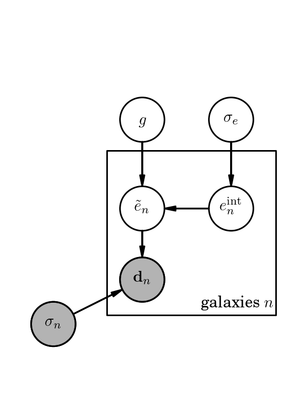
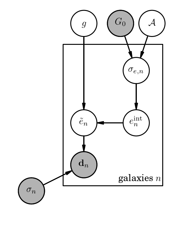
Figure 2.— Probabilistic graphical models for the two toy models in subsection 3.2. Left: Toy model 1 (subsubsection 3.2.1) is set up to illustrate how marginalizing over $\sigma_{e}$ reduces biases in the inferred shear $g$. Right: Toy model 2 (subsubsection 3.2.2) is set up to illustrate how marginalizing over possible distributions for $\sigma_{e}$ improves the marginal shear inference in cases where the intrinsic ellipticity is generated from multiple statistical populations.

For our toy models we introduce the following notation for ellipticities, $e^{\rm int}$ is intrinsic ellipticity in a galaxy model, $\tilde{e}$ is the galaxy model ellipticity after applying a shear $g$ to the model, $\varepsilon^{\rm obs}$ is an estimator for ellipticity computed from observed pixel values.

3.2.1 Toy model 1: Benefits of hierarchical inference

Marginalizing the parameters of the intrinsic galaxy ellipticity distribution can reduce biases in the shear inferences in some cases. We illustrate this point with a simple statistical model that we will refer to as ‘toy model 1’.

We construct a simplified model for the shear inference with the following assumptions:

1. the pixel data for each galaxy is reduced to ‘observed’ ellipticity components $\varepsilon^{\rm obs}$ with observational uncertainties described by uncorrelated Gaussian noise with variance $\sigma_{\rm obs}^{2}$ for all galaxies,

2. the intrinsic galaxy ellipticity $e^{\rm int}$ is generated from a zero-mean Gaussian distribution and is inferred with a similar hyper-prior,

3. we can work in the weak shear regime where $\tilde{e}\approx e^{\rm int}+g$.

We illustrate the dependencies of toy model 1 in the left panel of Figure 2. This model is simple enough that we can derive the marginal posteriors for both the shear and the intrinsic ellipticity variance analytically. We perform these derivations in the next subsection and then use the results to build some intuition about the benefits of hierarchical inference of distributions of intrinsic galaxy properties in subsubsection 3.2.1.

Marginal posteriors for toy model 1

Because the intrinsic (i.e., unsheared) galaxy shapes are always unknown, we first marginalize over $e^{\rm int}$ in any analysis. For this toy model, marginalizing over the intrinsic ellipticities for each galaxy yields a Gaussian marginal likelihood for the observed ellipticities of each galaxy given a common variance $\sigma_{e}^{2}$ for the intrinsic galaxy ellipticities,

$${\rm Pr}(\varepsilon^{\rm obs}|g,\sigma_{e}^{2}) \propto$$

$$\int d^{2}e^{\rm int} \mathcal{N}_{\varepsilon^{\rm obs}}\left(e^{\rm int}+g,\sigma_{\rm obs}^{2}\right)\cdot\mathcal{N}_{e^{\rm int}}\left(0,\sigma_{e}^{2}\right)$$

$$=\mathcal{N}_{\varepsilon^{\rm obs}}\left(g,\sigma_{\rm obs}^{2}+\sigma_{e}^{2}\right).$$ ((32))

The marginal likelihood for $n_{\rm gal}$ galaxies is just the product of $n_{\rm gal}$ versions of subsubsection 3.2.1,

$${\rm Pr}\left(\left\{\varepsilon^{\rm obs}_{i}\right\}_{i=1}^{n_{\rm gal}}|g,\sigma_{e}^{2}\right) \propto\prod_{i=1}^{n_{\rm gal}}{\rm Pr}(\varepsilon^{\rm obs}_{i}|g,\sigma_{e}^{2})$$

$$=\left(2\pi\sigma^{2}\right)^{-n_{\rm gal}/2} \exp\left[-\frac{n_{\rm gal}}{2\sigma^{2}}{\rm Var}\left\{\varepsilon^{\rm obs}_{i}\right\}\right]$$

$$\times\exp\left[-\frac{n_{\rm gal}}{2\sigma^{2}}\left|g-\bar{\varepsilon}^{\rm obs}\right|^{2}\right],$$ ((33))

where we defined,

$$\bar{\varepsilon}^{\rm obs}\equiv\frac{1}{n_{\rm gal}}\sum_{i=1}^{n_{\rm gal}}\varepsilon^{\rm obs}_{i},\quad{\rm and}\quad\sigma^{2}\equiv\sigma_{\rm obs}^{2}+\sigma_{e}^{2}.$$ ((34))

The conditional posterior for the shear $g$ is a Gaussian distribution given $n_{\rm gal}$ galaxy observations and a known (or assumed) value for the intrinsic ellipticity variance $\sigma_{e}^{2}$,

$${\rm Pr}\left(g|\sigma_{e}^{2},\left\{\varepsilon^{\rm obs}_{i}\right\}\right) \propto{\rm Pr}\left(\left\{\varepsilon^{\rm obs}_{i}\right\}|g,\sigma_{e}^{2}\right)\cdot\mathcal{N}_{g}\left(0,\sigma_{g}^{2}\mathbb{1}_{2}\right)$$

$$\propto\mathcal{N}\left(\mu_{cg},\sigma^{2}_{cg}\mathbb{1}_{2}\right)$$ ((35))

with,

$$\mu_{cg} \equiv\bar{\varepsilon}^{\rm obs}\left(1+\frac{\sigma^{2}}{n_{\rm gal}\sigma_{g}^{2}}\right)^{-1}$$ ((36))

$$\sigma^{2}_{cg} \equiv\frac{\sigma^{2}/n_{\rm gal}}{1+\frac{\sigma^{2}}{n_{\rm gal}\sigma^{2}_{g}}}.$$ ((37))

subsubsection 3.2.1 represents the shear posterior that is realized in any analysis that does not attempt to simultaneously infer the intrinsic ellipticity distribution. It is useful to consider some limiting cases of subsubsection 3.2.1.

Equation (36) suggests defining the composite variable,

$$x\equiv\frac{\sigma^{2}}{n_{\rm gal}\sigma_{g}^{2}}.$$ ((38))

Then,

$$\mu_{cg}=\frac{\bar{\varepsilon}^{\rm obs}}{1+x},\qquad\sigma^{2}_{cg}=\sigma_{g}^{2}\frac{x}{1+x}.$$ ((39))

So, point estimators for $g$ conditioned on $\sigma_{e}$ will become more biased towards zero as $x$ increases (e.g., for small numbers of galaxies, an informative zero-mean shear prior, or a large dispersion in the intrinsic galaxy ellipticities). The variance on the maximum posterior estimator for $g$ becomes arbitrarily small as $x\rightarrow 0$ (e.g., as $n_{\rm gal}\rightarrow\infty$) but is bounded from above by the value of $\sigma_{g}^{2}$ as $x$ becomes large.

Marginalizing over $\sigma_{e}^{2}$ in subsubsection 3.2.1 requires performing the integral,

$$\int_{0}^{\infty}dx\,(\sigma_{\rm obs}^{2}+x)^{b}\exp\left(-\frac{a}{\sigma_{\rm obs}^{2}+x}\right)\\ =a^{1-b}\gamma\left(b-1,\frac{a}{\sigma_{\rm obs}^{2}}\right),$$ ((40))

where $\gamma(b-1,a/\sigma_{\rm obs}^{2})$ is the lower incomplete Gamma function, and,

$$b \equiv n_{\rm gal}$$

$$a \equiv n_{\rm gal}{\rm Var}\left\{\varepsilon^{\rm obs}_{i}\right\}+n_{\rm gal}\frac{1}{2}\left|g-\bar{\varepsilon}^{\rm obs}\right|^{2}.$$ ((41))

Marginalizing over the shear gives the following posterior distribution for the intrinsic ellipticity variance,

$${\rm Pr}\left(\sigma_{e}^{2}|\left\{\varepsilon^{\rm obs}_{i}\right\},\sigma_{g}^{2}\right)\\ \propto\Gamma^{-1}\left(n_{\rm gal}-2,n_{\rm gal}\frac{1}{2}{\rm Var}\left\{\varepsilon^{\rm obs}_{i}\right\}\right)\\ \times\mathcal{N}_{\bar{\varepsilon}^{\rm obs}}\left(0,\sigma_{g}^{2}+\frac{\sigma^{2}}{n_{\rm gal}}\right),$$ ((42))

where $\Gamma^{-1}$ is the inverse-Gamma distribution.

We plot the expressions in Equations 3.2.1, (40), and (42) for the toy model 1 conditional and marginal posteriors in Figure 3. We have selected parameters for Figure 3, listed in Table 2, that illustrate how a large bias in the shear from the posterior conditioned on $\sigma_{e}^{2}$ can be alleviated by marginalizing $\sigma_{e}^{2}$. However, many combinations of parameters in toy model 1 will result in smaller shear biases.

Table 2Parameters for toy model 1 posterior plots

Parameter	Value
$g_{1,2}$	(0.05, -0.05)
$\sigma_{\rm obs}^{2}$	$7.6\times 10^{-5}$
$n_{\rm gal}$	100
$\sigma_{g}$	0.05
$\sigma_{e}$	$0.258$
bias in assumed $\sigma_{e}$	0.242

The value of $\sigma_{e}$ in Table 2 is derived from a Gaussian fit to the distribution of ellipticity values in the Deep Lens Survey (DLS) (Wittman et al., 2002; Jee et al., 2013) (with shear included, but after correction for the PSF). We assume 100 galaxies in Table 2 both because the shear may not be expected to be constant over a sky area containing larger numbers of galaxies, and because the GNU Scientific Library (Galassi, 2009) routine we use to evaluate Equation (40) does not yield numerically stable results for larger $n_{\rm gal}$ values.

The final line of Table 2 indicates the ‘bias’ in the value of $\sigma_{e}$ that is assumed in the conditional posterior in subsubsection 3.2.1, relative to the true value of $\sigma_{e}=0.258$. With this bias of $0.242$, the assumed value of $\sigma_{e}^{\rm assumed}=0.5$, indicating a value that might be chosen as ‘non-informative’ in a non-hierarchical analysis. Figure 3 then shows that knowledge of the true distribution of intrinsic ellipticities (via hierarchical inference) can be important in mitigating shear biases and it is not sufficient to assert a broad intrinsic ellipticity prior.

Prior choices for shear point estimators

Most published cosmic shear analyses rely on point estimators for the shear of each galaxy image. We do not advocate the use of point estimators for the shear. But in this subsection we consider the shear posterior mean as a possible point estimator that might be compared with other point estimators in the literature.

The mean of the shear conditional posterior, subsubsection 3.2.1, is least biased relative to the true shear when $\sigma_{g}$ is large and the true value of $\sigma_{e}$ is known. The mean of the marginal posterior for the shear, Equation (40), does not require knowledge of $\sigma_{e}$ since it has been integrated out and is similarly least biased when $\sigma_{g}$ is large. These statements of course depend on our assumption of a zero-mean shear prior.

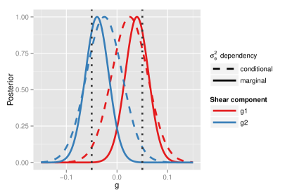
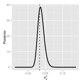
Figure 3.— Conditional and marginal posteriors for the shear and intrinsic ellipticity variance in toy model 1. The vertical dotted lines denote the values used to generate the data. See Table 2 for the parameter values used in this figure.

In Figure 4 we show the bias in the mean of the conditional shear posterior and in the marginal shear posterior as a function of $\sigma_{g}$ and the bias in the assumed value of $\sigma_{e}$ relative to the value used to generate the data. We can see that the relative bias (right panel of Figure 4) in the mean between the conditional and marginal shear posteriors is largest for large $\sigma_{g}$ and large assumed $\sigma_{e}$. One might have naïvely guessed that flat priors in shear and intrinsic ellipticity (equivalent in our toy model to large $\sigma_{e}$ and $\sigma_{g}$) would be the obvious choice for shear inference in the absence of any other information. But, Figure 4 illustrates that such flat priors will give the most biased shear inference relative to what could be obtained with a hierarchical model for the intrinsic galaxy ellipticities.

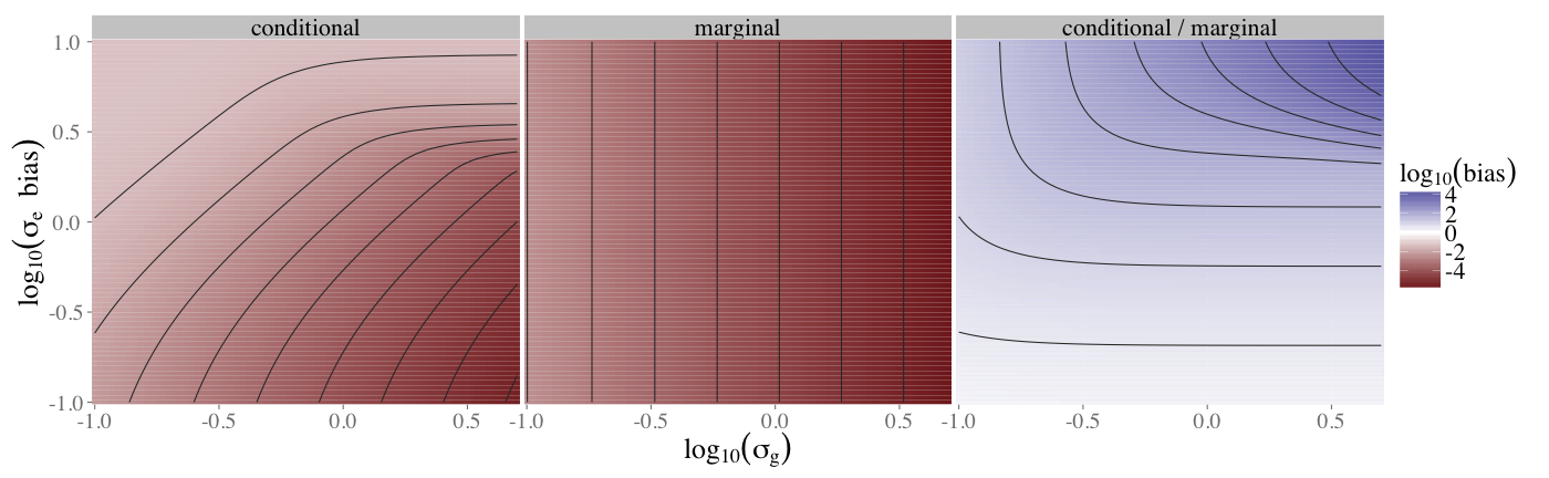
Figure 4.— Biases in the posterior means for a component of the shear. The left panel shows the posterior mean bias when conditioned on the assumed width of the intrinsic ellipticity distribution, $\sigma_{e}$. The central panel shows that of the posterior marginalized over $\sigma_{e}$ (which is insensitive to biases in assumed $\sigma_{e}$). The right panel is the ratio of the shear biases in the left and central panels. The vertical axis shows the logarithm of the additive bias in the assumed $\sigma_{e}$ relative to the true value (so a perfect guess for the true width of the intrinsic ellipticity distribution corresponds to $-\infty$ on the vertical axis). The horizontal axis shows the logarithm of the width of the zero-mean prior for the shear components. For all assumed values of $\sigma_{e}$ and $\sigma_{g}$, marginalizing over $\sigma_{e}$ always gives less biased shear posterior means (comparing the central to the left panel). In addition, assuming broad priors (i.e., weakly informative) for the intrinsic ellipticity and the shear gives the most biased shear inferences if one does not marginalize over the intrinsic ellipticity distribution width (right panel).

3.2.2 Toy model 2: DP inference given a bimodal intrinsic ellipticity distribution

We now construct a numerical toy model to illustrate how the marginal shear inference can be improved by taking advantage of the flexibility of the DP as a conditional PDF for the distribution of intrinsic galaxy properties instead of asserting a simple Gaussian distribution for the galaxy properties. We will refer to the models in this subsection collectively as ‘toy model 2’.

As in toy model 1, we assume the pixel data is reduced to observed ellipticities. Unlike in toy model 1 we no longer assume weak shear or a fixed correspondence between the intrinsic ellipticity generating distribution and PDF for inference.

Our objective with toy model 2 is to compare the marginal shear and ellipticity inferences when using either a restrictive or flexible conditional PDF for $\sigma_{e}^{2}$, irregardless of the generating distribution for the data.

For a restrictive PDF, we specify a uniform prior on a single $\ln(\sigma_{e})$ parameter for all galaxies, effectively assuming that all galaxy ellipticities are drawn from a common zero-mean Gaussian distribution. We call this PDF choice our ‘Gaussian’ model. We use the DP model for $\sigma_{e}^{2}$ as a flexible hierarchical PDF specification, which we label as our ‘DP’ model. We describe each model in Table 3.

Table 3Intrinsic ellipticity PDFs for toy model 2.

Model	${\rm Pr}(e^{\rm int}_{i})$	${\rm Pr}(\sigma_{e}^{2})$
Gaussian	$N\left(0,\sigma_{e}\right)$	$1/\sigma_{e}^{2}$
DP	$N\left(0,\sigma_{e,i}\right)$	${\rm DP}(\mathcal{A},G_{0})$

Figure 2 shows the relationships of the parameters in the Gaussian and DP models (left and right panels).

To test and compare the ‘Gaussian’ and ‘DP’ models (distinct from the prescription for generating data) we generate two mock data sets, each with 100 galaxies. For each data set we draw samples of $e^{\rm int}$ from a two-component Gaussian mixture,

$${\rm Pr}(e^{\rm int})=\lambda\mathcal{N}(0,\sigma_{e,1})+(1-\lambda)\mathcal{N}(0,\sigma_{e,2}),$$ ((43))

with parameters given in Table 4.

Table 4Mock data parameters for toy model 2.

Data set	$\sigma_{e,1}$	$\sigma_{e,2}$	mixture fraction $\lambda$
Unimodal	0.258	0	1
Bimodal	0.258	0.03	0.7

The ‘unimodal’ data set has $\lambda=1$ indicating the $e^{\rm int}$ samples are drawn from a single Gaussian distribution (matching the distribution in toy model 1). For the ‘bimodal’ data set, we draw $e^{\rm int}$ from a bimodal distribution with 70% of galaxy ellipticities sampled from the Gaussian with width matching that of the unimodal data set, and 30% sampled from a much narrower distribution of intrinsic ellipticity. We describe our detailed procedure for generating mock data sets in Appendix D. Figure 5 shows the observed ellipticity components generated for each mock data set.

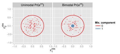
Figure 5.— Mock data for 100 simulated galaxy ellipticities for toy model 2. The intrinsic ellipticity components are generated from two-component Gaussian mixture models with parameters given in Table 4.

We motivate the values of $\sigma_{e,1}$ and $\sigma_{e,2}$ in Table 4 by fitting one- or two-component Gaussian mixtures to the distribution of observed ellipticities from the Deep Lens Survey (DLS) (Jee et al., 2013). These ellipticities have been PSF corrected, but include the cosmic shear. We find that a two-component Gaussian mixture is a better fit to the observed ellipticity distribution, giving some motivation for the two-component mixture in our bimodal data set. However, in Table 4 we have artificially increased the fraction of galaxies with a narrow ellipticity distribution over that found in the DLS (where we find a mixture fraction of $\sim 90\%$ for the broader ellipticity distribution).

Figure 6 shows the marginal posteriors for the shear and the intrinsic ellipticity variance as estimated from MCMC samples. We describe the conditional distributions for Gibbs sampling the DP model parameters for toy model 2 in Appendix E. We note here however, that since we have not yet specified an algorithm to determine the DP hyperprior parameters $\tau$ and $m$ (see equation B4 and surrounding discussion), we have assigned informative priors for these parameters that are different for the unimodal and bimodal data sets given our knowledge of the generating distributions. An important area for future work will be to dynamically set or sample in the hyperprior parameters for the DP base distribution.

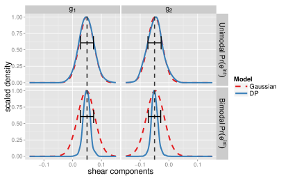
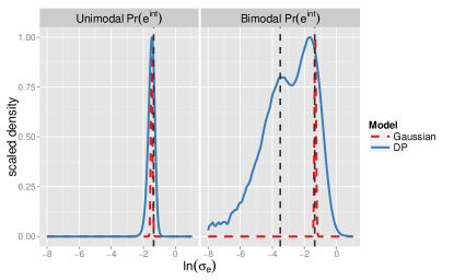
Figure 6.— Top: Marginal posteriors for the shear components under the four toy model 2 scenarios. The horizontal black lines with error bars indicate the mean and uncertainty on the shear estimator obtained from averaging the observed ellipticity components of all galaxies. Bottom: Marginal posteriors for the logarithm of the standard deviation parameter in the intrinsic ellipticity distribution. For the DP model, we compute marginal densities from the concatenation of MCMC samples for $\sigma_{e,i}$ with $i=1,\dots,n_{\rm gal}$. The vertical dashed lines in all panels show the ‘true’ values corresponding to the circles in Figure 5.

The horizontal black lines in the top panel of Figure 6 indicate the uncertainty on the naïve shear estimator obtained by averaging the observed ellipticities of the galaxies (i.e., the horizontal line gives sd$\left(\left\{\varepsilon^{\rm obs}_{i}\right\}_{i=1}^{n_{\rm gal}}\right)/\sqrt{n_{\rm gal}})$. These naïve shear estimator lines are positioned at the hieght of the 1-$\sigma$ width of the posterior densities for each model.

Table 5Ratios of mean marginal shear biases using the DP or Gaussian models to marginalize the intrinsic ellipticities for toy model 2.

Data set	DP model / Gaussian model
	$(g_{1},g_{2})$
Unimodal	(1.26, 1.23)
Bimodal	(0.46, 0.12)

For the marginal shear posteriors with the unimodal data set (top row of the top panel in Figure 6), both the Gaussian and DP models yield similar results, which are similar as well to results obtained using a simple average of the ellipticities to estimate the shear.

However, the shear marginals for the bimodal data set (lower row of the top panel of Figure 6) show large differences between the Gaussian and DP models. The Gaussian model yields shear marginal distributions similar to those obtained with the unimodal data set, while the DP model yields shear marginals that are more than twice as precise as those assuming the Gaussian model (and are narrower than the shear errors obtained from averaging ellipticities). In Table 5 we give the ratio of the biases in the mean $g_{1},g_{2}$ from the DP model to that from the Gaussian model for each of the mock data sets. For the bimodal data set, the DP model yields mean shear estimates that are less biased than the Gaussian model, while the reverse is true for the unimodal data set. These results are better understood by next investigating the $\sigma_{e}$ marginal distributions in the lower panel of subsection 3.2.

For the unimodal data set, both models yield accurate inferences of $\sigma_{e}$, although the DP model gives a broader marginal posterior than the Gaussian model. However, for the bimodal data set (right half of the lower panel of subsection 3.2, the Gaussian model yields a tight posterior for $\sigma_{e}$ that misses the existence of a sub-population of galaxies generated from a much narrower intrinsic ellipticity distribution. The DP model yields a bimodal marginal posterior for $\sigma_{e}$, indicating some knowledge of the bimodal nature of the generating distribution.

We can now understand the marginal shear posteriors given the bimodal data set as follows. The Gaussian model effectively assumes the entire galaxy population is generated from a broad intrinsic ellipticity distribution, which limits the precision with which the shear can be measured. The widths of the the Gaussian model shear marginals given the unimodal and bimodal data sets are similar because the inference assumes similar width ellipticity generating distributions. However, because the DP model accurately infers the existence of a galaxy sub-population with small intrinsic ellipticities, this information can be used to more precisely infer the shear for the whole population.

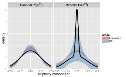
Figure 7.— Realizations of the intrinsic ellipticity distribution given marginal posterior samples of $\sigma_{e}$ in toy model 2. The black lines show the generating distributions for mock data scenarios ‘data1’ and ‘data2’. The shaded bands indicate the 68% credible intervals on the realized ellipticity probability densities. In both mock data scenarios, the credible interval for ‘model1’, which assumes $\sigma_{e}$ is the same for all galaxies, excludes the generating distributions.

Figure 7 shows another way to visualize and interpret the inferences of the intrinsic ellipticity distributions with both models. The solid lines in Figure 7 show the generating distributions of $e^{\rm int}$ for the unimodal and bimodal data sets. The shaded bands show the 68% credible intervals for the inferred $e^{\rm int}$ distributions given marginal posterior samples of $\sigma_{e}$ from both models. While the shaded band for the Gaussian model is not dissimilar from the generating distribution for the unimodal data set, it is a poor approximation to the generating distribution for the bimodal data set. We should therefore expect larger shear errors and biases when using the Gaussian model to analyze the bimodal data set than when using a more flexible ellipticity conditional PDF as in the DP model.

In the case of the bimodal generating distribution, we might obtain more precise and accurate marginal shear inferences from a model for the intrinsic ellipticity distribution that is still unimodal, but calibrated from a sub-sample of the data to partially include information about a rounder subpopulation of galaxies with a different response to shear. The real power of the DP, however, is that it not only helps to infer the underlying distribution of intrinsic ellipticities from the data but that it also enables assigning different galaxies to different latent classes. Thus, it is capable of determining which galaxies to weight more in the shear measurement (i.e., those that belong to classes with smaller intrinsic ellipticity variance). The DP inference thereby results in not only a less biased shear inference but also a more precise shear inference.

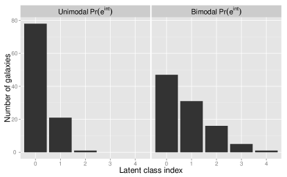
Figure 8.— The number of galaxies assigned to each of the DP latent classes for a single sample from the MCMC chains for the ‘data1’ and ‘data2’ mock data scenarios in toy model 2. More galaxies assigned to latent classes with larger indices (starting from 0) indicate more distinct clusters of galaxy ellipticities are favored by the DP model.

We can also draw some insight about the galaxy population from the DP sampling in the DP model. The two peaks in the $\sigma_{e}$ marginal distribution in Figure 6 indicate the presence of two populations of galaxies with different intrinsic ellipticity distributions in the bimodal data set. We can draw a similar conclusion from the samples of the latent class selectors in the DP model as defined in Equation (24). Figure 8 shows the distributions of latent class indices (given integer labels increasing from 0) for a single sample from the the DP model MCMC chains. We see that the posterior samples given the unimodal data set indeed favor a single generating distribution while those for the bimodal data set favor more than one generating distribution. The shear inference in all cases is marginalized over these latent class assignments.

4. Discussion and conclusions

4.1. Hierarchical inference for PSFs and shear

With the toy models in Section 3 we demonstrated how to simultaneously infer a constant shear and the intrinsic galaxy ellipticities. We generated interim posterior samples for each galaxy independently and then combined the inferences from each galaxy using importance sampling and a DP model for the intrinsic ellipticity distribution. By specifying a common hierarchical conditional PDF on the parameters of the intrinsic ellipticity distribution for the galaxy population, we statistically correlated, and thereby improved, the marginal shear inference given all galaxies. A key feature of our model for the intrinsic ellipticity PDF is the assignment of galaxies into latent classes based on the inferred intrinsic ellipticity variance. This allows an improved sensitivity to the action of shear on galaxies with different intrinsic ellipticity magnitudes.

Extending the statistical model to that presented in Equation (18) to include inference of the PSF and shear that is allowed to vary over the sky will have similar effects in correlating the inferences from each galaxy at a hierarchical level. As an aside, the hierarchical model that imposes parameters common to all galaxies in the PDF on, e.g., the intrinsic ellipticity is what allows us to perform interim posterior sampling on individual galaxies as in subsubsection 2.2.2. Similar conclusions hold for both the marginalization of the intrinsic galaxy properties $\omega$ and the lensing potential $\psi$.

The shear is correlated across sky positions because of the common gravitational potentials that distort the light from different galaxies. Ideally, then, we would like to infer the 3D matter potential $\Psi$ from the combination of galaxy shears and redshift information and infer cosmology from the statistics of the 3D mass distribution. While the initial conditions for the 3D mass distributions can be modeled as Gaussian distributed to good approximation, the late-time mass distribution is non-Gaussian and includes significant correlations between Fourier modes of the density field. It is not obvious how to specify a conditional PDF on the 3D mass distribution or how to feasibly sample model parameters (see, e.g., Schneider et al., 2011, for an approach to using cosmological $N$-body simulations for this purpose). Jasche & Wandelt (2013) and Jasche et al. (2014) have presented reconstructions of the 3D mass density and cosmological initial conditions from galaxy clustering inferred in a spectroscopic survey that might become useful for shear inference as well in the future.

If we pursue a description of the mass density in terms of the realization of the cosmological initial conditions as in Jasche et al. (2014), then we would infer cosmological parameter constraints by marginalizing the initial conditions $\Psi^{\rm initial}$. The lens potential realizations for different source distributions $s$ all depend on the same initial conditions realization $\Psi^{\rm initial}$ evolved under the same cosmology $\bm{\theta}$. So, when we marginalize the initial conditions realization $\Psi^{\rm initial}$ the distributions of $\psi_{s}$ are no longer separable for different $s$. This is consistent with the common intuition that the lens potentials for, e.g., different photo-$z$ bins, should be correlated by common lensing mass along the lines of sight. This is also why the probability distribution of $\{\psi_{s}\}$ for all source distributions $s$ does not factor over $s$ in Equation (18).

4.2. No more point estimators for galaxy catalogs

In traditional algorithms, point estimators for the ellipticity of an individual galaxy can be computed from a ‘postage stamp’ image of the galaxy isolated from the rest of the survey imaging. The ellipticity estimates from individual galaxies can then be averaged over local regions of the sky to estimate the shear.

Our likelihood in Equation (9) also applies to galaxy ‘postage stamps’. But, there is no statistically meaningful method to combine the information from individual postage stamps unless we draw interim posterior samples from each postage stamp and use methods such as in subsubsection 2.2.2. We come to an important conclusion then that we should dispense with computing point estimators from postage stamp images of galaxies for the purposes of later model inferences (this point was also made previously in Brewer et al., 2013; Hogg, 2012).

4.3. Conclusions

We have described a hierarchical statistical framework to infer cosmic shear from galaxy imaging surveys. By explicit specification and marginalization of the statistical models for intrinsic (i.e., unlensed) galaxy properties and the PSF, we may be able to improve both the accuracy and precision of the shear inference over previously published algorithms. With a simple toy model in Section 3 we showed promising improvements in the precision of the marginal shear inference when galaxy ellipticities are generated from a bimodal distribution (intended to mimic the different morphological classes of observed galaxies).

We assume a likelihood function for the imaging pixel data. Because we estimate ellipticities and shears as galaxy model parameters rather than reduced statistics of the data, defining a likelihood for pixel values poses no algorithmic challenges for our framework over using reduced statistics. With an importance sampling algorithm we can infer model parameter constraints for independent galaxy images and combine these inferences into a consistent shear inference over many galaxies. We are only able to perform this importance sampling mathematically by means of a hierarchical model that relates the inferences from individual galaxies by means of common parameters in the distributions over galaxy properties and PSFs. Our framework also strongly motivates the use of random samples of posterior model parameters rather than point estimators for constructing source catalogs for cosmic shear analysis.

We also introduced a random process to model the distribution of intrinsic galaxy properties (such as ellipticity and size). Our Dirichlet Process (DP) model can fit a wider range of distributions than any asserted specific functional form. In subsubsection 3.2.2 we showed that biased inference of, e.g., the intrinsic galaxy ellipticity distribution can be another form of ‘model fitting bias’ in the marginal shear constraints. Our DP model helps in alleviating the bias in the posterior median shear (e.g., Table 5) when the generating distribution is multi-modal, but is even more important in reducing the posterior uncertainty on the shear (Figure 6). When we assume a single Gaussian for the generating distribution of galaxy ellipticities the DP model yields shear inferences that are more biased and no more precise than assuming a Gaussian prior on the ellipticities (the Gaussian model with the unimodal data set in toy model 2 of subsubsection 3.2.2). However, this scenario is a limiting case in that we do not expect the distribution of properties of the galaxy population to be well-described by a unimodal Gaussian distribution, and we do not expect to be able to perfectly match our model distribution to the true generating distribution. The similar marginal shear inferences we obtain with flat or DP ellipticity variance PDFs for the unimodal data set in our toy model is therefore a validation of our DP model distribution, which can still perform well when the generating distribution for galaxy ellipticities is more complex. An important topic to explore further is algorithmic determination of all hyper-prior parameters in the DP model.

While we believe the importance sampling and DP algorithms we presented will be useful for the analysis of upcoming large surveys, considerable work remains in implementing variations of these algorithms for large-scale imaging analysis.

Bard et al. (in prep.) shows that our interim posterior sampling given galaxy pixel data is computationally limited both by galaxy model parameter optimizations and by MCMC sampling. Future developments in fast analytic models for galaxy profiles could reduce the computational requirements at this step. The model in Spergel (2010) is an intriguing example of such model variations worth exploring. We also speculate that conventional model-fitting biases, resulting from galaxy models that cannot describe all important features in the data, may be partially alleviated by a flexible model for the PDF on the galaxy model parameters. Because both a change of galaxy model and a change of conditional PDF on a given galaxy model are changes in the integration measure when marginalizing intrinsic galaxy properties it is possible that a suitable conditional PDF specification can reduce remaining model fitting biases.

Our implemention of DP parameter inference relies on Gibbs sampling, which must proceed sequentially in all model parameters. This sampling can become a computational bottleneck as the number of latent classes increases in the DP (with a corresponding increase in the number of parameters to Gibbs update). Parallelizing the Gibbs updates may become useful in cases where the number of latent classes is large. However, optimizing the computational performance of the DP sampling is an area for future work.

Our framework also offers interesting possibilities to infer the distribution of intrinsic galaxy properties (conditioned on some galaxy modeling assumptions), after marginalizing over the shear and PSF. Again, work remains to remove any ad-hoc assumptions in the DP model to obtain confidence in any inferences about galaxy model parameters that are independent of implicit prior assumptions. That is, we want want to only impose explicit prior information about the galaxy properties without biases imposed by modeling limitations.

Finally, we must still demonstrate the PSF inference and marginalization using our framework with pixel-level image simulations. This capability is already part of The Tractor code that we use in Bard et al. (in prep.), but we have not propagated PSF uncertainties to the shear inference. We are also pursuing methods to incoporate ancillary information about the PSF (e.g., from site-monitoring data, wavefront sensors, or engineering images) using the framework in this paper.

Appendix A Modeling galaxy images

To evaluate the likelihood of the pixel values in Equation (9) we require a computationally efficient code to predict pixel values given a galaxy model that can be sheared, convolved with a given PSF, and depositied on pixels with the addition of noise. The Tractor public code performs exactly these operations. A key feature of The Tractor is that both galaxy flux and PSFs are represented as sums of 2D Gaussian distributions allowing fast analytic convolutions of model galaxy images with a model PSF.

For an isolated galaxy image (or “postage stamp”), we generate posterior samples of the galaxy model parameters $\omega$ via MCMC using The Tractor to evaluate the likelihood at each MCMC step (Bard et al., in prep.). In all tests of our algorithms we have used the public MCMC code emcee (Foreman-Mackey et al., 2013) for inferring galaxy model parameters and PSFs.

As we discuss in Bard et al. (in prep.), the initialization of the galaxy model parameters via numerical optimization can be the least accurate part of the calculation to infer posterior constraints on a galaxy model. We have found that an informed choice of ‘interim prior’ on the galaxy model can significantly improve the inferences for individual galaxies.

In the next sub-section we describe how to properly incorporate the posterior samples for individual galaxy models with per-galaxy interim prior information into the global statistical inference for a survey of galaxies. We reserve all further discussion of fitting galaxy models to pixel data to Bard et al. (in prep.).

Appendix B Choosing a base distribution for the intrinsic galaxy properties

We can further understand some of the choices in specifying a DP base distribution $G_{0}$ by considering the model where

$${\rm Pr}(\omega|\alpha)=\mathcal{N}_{\omega}(0,\mathsf{\Sigma})$$ (B1)

such that

$$\alpha\equiv\mathsf{\Sigma}$$ (B2)

is the (co)variance of the distribution of intrinsic galaxy properties.

In the case that $\omega_{n}$ is a single parameter so that $\mathsf{\Sigma}\equiv\sigma^{2}$, an obvious conjugate prior for $\sigma^{2}$ is the inverse-Gamma (IG) distribution. However, it is difficult to specify a non-informative prior on $\sigma^{2}$ using the IG distribution when the values of $\sigma^{2}$ are likely to be much less than one. Another choice is the uniform distribution, but this too often leads to biased inference of the variance parameter (Gelman, 2006).

Instead we follow Gelman (2006) and impose a more flexible, but still conditionally conjugate, distribution on $\sigma^{2}_{i}$ by decomposing $\omega_{i}=\left|\xi_{i}\right|\eta_{i}$, where $\xi$ is a scaling parameter and $\eta_{i}\sim\mathcal{N}(0,\sigma_{\eta}^{2})$. We specify distributions $\xi_{i}\sim\mathcal{N}(m,\tau^{-1})$ and $\sigma_{\eta}^{2}\sim{\rm DP}(\mathcal{A},G_{0})$. The standard deviation parameter is $\sigma=|\xi|\sigma_{\eta}$. The DP base distribution (now for $\sigma_{\eta}^{2}$) is,

$$G_{0}(\sigma^{2}_{\eta})=\Gamma^{-1}(a_{\eta},0.5).$$ (B3)

The family of distributions parameterized by $a_{\eta},m,\tau$ is quite flexible (Murugiah & Sweeting, 2012). To recover a simpler half-Cauchy PDF we take $m=0$ so that

$${\rm Pr}\left(\sigma^{2}|\tau,a_{\eta}\right)\propto\left(1+\tau\sigma^{2}\right)^{-(1+a_{\eta})},$$ (B4)

which illustrates how the scaling parameter precision $\tau$ affects the width of the base distribution for $\sigma$.

It is possible to generalize the above ‘variable expansion’ to a covariance $\mathsf{\Sigma}$ of a multivariate parameter vector $\omega_{n}$ of galaxy intrinsic properties.

Scaling parameter

To complete the specification of the statistical framework when the intrinsic galaxy properties are assumed Gaussian distributed, we derive the conditional posterior for $\xi$ after marginalizing over the galaxy properties $\omega$,

$${\rm Pr}(\xi_{n}|{\mathbf{d}},\sigma_{\eta,n},m,\tau,\psi)\propto{\rm Pr}\left(\xi_{n}|m,\tau\right)\int d\omega_{n}\,{\rm Pr}\left({\mathbf{d}}_{n}|\omega_{n}=(\eta_{n}\left|\xi_{n}\right|),\psi\right){\rm Pr}(\eta_{n}|\sigma_{\eta,n}^{2}),$$ (B5)

where again we assume $\omega_{n}$ is univariate for simplicity of presentation. Changing integration variables to $\eta_{n}=\omega_{n}/\left|\xi_{n}\right|$, allows us to use the previous importance sampling result (equation (15)) for the marginal likelihood after including the Jacobian for the variable transformation,

$${\rm Pr}(\xi_{n}|{\mathbf{d}},\sigma_{\eta,n},m,\tau,\psi)\propto{\rm Pr}\left(\xi_{n}|m,\tau\right)\frac{1}{N}\sum_{k=1}^{N}|\xi_{n}|\frac{{\rm Pr}\left(\eta_{nk}\equiv\omega_{nk}/\xi_{n}|\sigma_{\eta,n}^{2}\right)}{{\rm Pr}\left(\omega_{nk}|I_{0}\right)}.$$ (B6)

We use Equation B6 to conditionally update the values of the scaling parameters $\xi_{n}$ in our MCMC algorithm.

Appendix C Sampling the DP clustering parameter

In many applications (including ours) there is no obvious choice for the value of the DP clustering parameter $\mathcal{A}$. Instead, we marginalize over $\mathcal{A}$ with a suitably chosen prior.

Following Dorazio (2009) and Murugiah & Sweeting (2012) we place a conjugate Gamma prior on $\mathcal{A}$ so we can perform Gibbs updates. Dorazio (2009) presents a useful algorithm to determine the hyperparameters $(a,b)$ of the Gamma prior on $\mathcal{A}$ when little information is known about the expected number of clusters in the data (i.e., the number of morphologically distinct galaxy populations).

However, given the extensive existing research into galaxy formation (e.g., the common classifications of ‘early’ and ‘late’ type galaxies), we are motivated to place a more informative prior on $\mathcal{A}$. Murugiah & Sweeting (2012) describe several algorithms to determine the parameters $(a,b)$ for the Gamma prior on $\mathcal{A}$ in informative scenarios. We can impose our prior knowledge that there are early- and late-type galaxies by requiring the expected mean value of the number of clusters in the DP to be 2. Using the formula from Antoniak (1974),

$${\rm E}(M|n_{\rm gal},\mathcal{A})\approx\mathcal{A}\ln\left(\frac{n_{\rm gal}+\mathcal{A}}{\mathcal{A}}\right),$$ (C1)

for $n_{\rm gal}\gg 1$, and where $M$ is the number of clusters or latent classes in the DP. By solving Equation C1 for the value $\bar{\mathcal{A}}$ that gives the expected number of clusters, we set the Gamma prior parameters as,

$$a=\bar{\mathcal{A}}X,\qquad b=X,$$ (C2)

so that the prior mean of $\mathcal{A}$ is $a/b=\bar{\mathcal{A}}$ and the prior variance is $a/b^{2}=\bar{\mathcal{A}}{X}$ such that larger $X$ communicates more certainty on the expected number of morphological classes in the galaxy population. Murugiah & Sweeting (2012) present other algorithms to encode prior information on $\mathcal{A}$ that we reserve for future exploration.

Given the hyperprior parameters $(a,b)$, we perform Gibbs updates of $\mathcal{A}$ with the conditional distribution from Escobar & West (1995) (their eq. 13),

$$\mathcal{A}|\zeta,k\sim\pi_{\zeta}\Gamma(a+k,b-\log(\zeta))+\left(1-\pi_{\eta}\right)\Gamma\left(a+k-1,b-\log(\zeta)\right)$$ (C3)

where $k$ is the number of latent classes currently assigned to the data, and

$$\pi_{\zeta}\equiv\frac{a+k-1}{a+k-1+n_{\rm gal}(b-\log(\zeta))},$$ (C4)

with

$$\zeta|\mathcal{A}\sim\beta\left(\mathcal{A}+1,n_{\rm gal}\right),$$ (C5)

a variable used only in the Gibbs updates of $\mathcal{A}$, and $\beta$ denotes the Beta distribution.

Appendix D Generating fake posterior samples of galaxy ellipticities

For our ‘toy model 2’ in subsubsection 3.2.2 we generate fake summary statistics of galaxy pixel data with the following procedure:

1. Specify a value for the true reduced shear $g$ for all galaxies (we assume a constant shear for all galaxies in our numerical examples).

2. For each galaxy $i=1,\dots,n_{\rm gal}$, draw intrinsic ellipticities from a specified distribution $e^{\rm int}_{i}\sim{\rm Pr}_{e,{\rm true}}(\cdot)$.

3. Define the complex ellipticity of the generative model for the pixel data for each galaxy by transforming the intrinsic ellipticity $e^{\rm int}$ with the shear $g$,

   $$\tilde{e}_{i}=\frac{e^{\rm int}_{i}+g}{1+g^{*}e^{\rm int}_{i}}.$$ (D1)

Given the observed ellipticity as a summary statistic of the pixel data, we generate interim posterior samples of the galaxy ellipticity by:

1. Define an interim prior for the model ellipticity ${\rm Pr}_{\rm interim}(\tilde{e}_{i})$. This prior may be chosen for computational convenience rather than an accurate description of the data, with the knowledge that we will re-weight the posterior samples later to accomodate a hierarchical PDF on the intrinsic ellipticity $e^{\rm int}_{i}$.

2. Define a summary statistic of the pixel data for a galaxy $\varepsilon_{i}$ and a functional form for the likelihood ${\rm Pr}\left(\varepsilon_{i}|\tilde{e}_{i}\right)$ of the summary statistic.

3. Draw samples from the interim posterior,

   $${\rm Pr}(\tilde{e}_{i}|\varepsilon_{i})\propto{\rm Pr}(\varepsilon_{i}|\tilde{e}_{i}){\rm Pr}_{\rm interim}(\tilde{e}_{i}).$$ (D2)

The samples of $\tilde{e}_{i}$ contain all the statistical information about galaxy $i$. For extreme data compression we might limit ourselves to one sample of $\tilde{e}_{i}$ for each galaxy.

Appendix E DP sampling algorithm for toy model 2

After marginalizing over the intrinsic ellipticity components, the posterior $\mathcal{H}_{n}$ for the intrinsic ellipticity variance given a single galaxy $n$ is (assuming weak shear, $g\ll 1$),

$$\mathcal{H}_{n}(\sigma_{\eta}^{2}|\xi_{n},{\mathbf{d}}_{n},g) =G_{0}(\sigma_{\eta}^{2})\int d^{2}\eta\,{\rm Pr}({\mathbf{d}}_{n}|g,\xi,\eta)\cdot{\rm Pr}(\eta|\sigma_{\eta}^{2})$$

$$=\frac{(0.5)^{a_{\eta}}}{\Gamma(a_{\eta}}\left(\sigma_{\eta}^{2}\right)^{-(1+a_{\eta}}\exp\left(-\frac{0.5}{\sigma_{\eta}^{2}}\right)$$

$$\times\frac{1}{2\pi\left(\sigma_{\rm obs}^{2}+\xi_{n}^{2}\sigma_{\eta}^{2}\right)}$$

$$\times\exp\left(-\frac{1}{2}\frac{\left(d_{n,1}-g_{1}\right)^{2}+\left(d_{n,2}-g_{2}\right)^{2}}{\sigma_{\rm obs}^{2}+\xi_{n}^{2}\sigma_{\eta}^{2}}\right).$$ (E1)

This expression is pedagogical only. In practice, we do not have ${\mathbf{d}}_{n}$ values. Instead we have importance samples of $e^{\rm int}\equiv|\xi|\eta$ with which we perform the above integral via Monte Carlo.

Following from Equation (21) and Neal (2000), the conditional posterior for $\sigma^{2}_{\eta,n}$ for galaxy $n$ is,

$$\sigma^{2}_{\eta,n}|\sigma^{2}_{\eta,-n},{\mathbf{d}}_{n}\sim\sum_{m\neq n}q_{n,m}\delta_{\rm D}\left(\sigma^{2}_{\eta,m}\right)+r_{n}\mathcal{H}_{n}$$ (E2)

where $\delta_{\rm D}(\sigma^{2}_{\eta,m})$ is a Dirac delta function indicating that $\sigma_{\eta,n}^{2}$ for galaxy $n$ takes the same value as that for galaxy $m$. This is how clustering occurs in the Gibbs sampling. The coefficient of the delta functions $q_{n,m}$ is defined to be the marginal likelihood for galaxy $n$ given the parameter $\sigma^{2}_{\eta,m}$ currently assigned to galaxy $m$,

$$q_{n,m}=b\int d^{2}\eta\,{\rm Pr}({\mathbf{d}}_{n}|\eta,\xi_{m},g)\cdot{\rm Pr}(\eta|\sigma^{2}_{\eta,m}),$$ (E3)

where $b$ is a constant defined below. If all the $q_{n,m}\forall m\neq n$ are sufficiently small, meaning that no parameters $\sigma^{2}$ currently assigned to other galaxies are good descriptions of observation $n$, then we draw a new value for $\sigma_{\eta,n}^{2}$ from $H_{n}$. The coefficient that defines the probability for drawing new values relative to the coefficients $q_{n,m}$ is the likelihood for galaxy $n$ marginalized over both the intrinsic ellipticity components and the hyperprior parameter $\sigma_{\eta}^{2}$,

$$r_{n}=b\,\mathcal{A}\int d\sigma_{\eta}^{2}\,\int d^{2}\eta\,{\rm Pr}({\mathbf{d}}_{n}|\eta,\xi_{n},g)\cdot{\rm Pr}(\eta|\sigma_{\eta}^{2})\cdot G_{0}(\sigma_{\eta}^{2}|a_{\eta}).$$ (E4)

Note that $r_{n}$ is proportional to $\mathcal{A}$ so that larger $\mathcal{A}$ values mean less clustering of $\sigma_{\eta,n}^{2}$ values for each galaxy.

The parameter $b$ is defined so that

$$\sum_{m\neq n}q_{n,m}+r_{n}=1.$$ (E5)

Given the importance samples for $e^{\rm int}$, we compute $q_{n,m}$ as,

$$\frac{1}{b}q_{n,m}=\frac{1}{K}\sum_{k=1}^{K}\frac{{\rm Pr}(e^{\rm int}_{kn}/\xi_{n}|\sigma^{2}_{\eta,m})}{{\rm Pr}_{\rm interim}(e^{\rm int}_{kn})}$$ (E6)

Similarly, we compute $r_{n}$ by first integrating analytically over $\sigma_{\eta}^{2}$ and then summing over the $e^{\rm int}$ samples,

$$\frac{1}{b}r_{i}=\frac{1}{K}\sum_{k=1}^{K}\frac{{\rm Pr}_{\rm marg}(e^{\rm int}_{kn}/\xi_{n}|a_{\eta})}{{\rm Pr}_{\rm interim}(e^{\rm int}_{kn})},$$ (E7)

where, assuming the parameter $m=0$ as in Equation B4,

$${\rm Pr}_{\rm marg}\left(\eta|a_{\eta}\right) \equiv\frac{0.5^{a_{\eta}}}{2\pi}\frac{\Gamma(1+a_{\eta})}{\Gamma(a_{\eta})}\left(\frac{1}{2}\left(1+|\eta|^{2}\right)\right)^{-(1+a_{\eta})}$$ (E8)

and $a_{\eta}$ is a parameter in the inverse Gamma base distribution $G_{0}$ as defined in Equation B3.

Appendix F Galaxy moments as summary statistics of the pixel data

Bernstein & Armstrong (2014) (BA14) recently enumerated the challenges in modeling galaxy images at the pixel level because of the sensitivity to unknown features in complex galaxy morphologies. Throughout this paper we have assumed we can find a parameterized model for the galaxy morphologies that is sufficiently descriptive and flexible to avoid large model fitting biases. However we have not described and validated such a model and it remains possible that model-fitting biases will remain a significant challenge within our statistical framework.

In this appendix we consider the approach in BA14 and assume the galaxy pixel data is compressed into a set of moments. We will demonstrate that there can be stringent requirements on the prior knowledge of the galaxy moments that are not obviously easier to satisfy than the pixel-level model specification we assume in the main body of our paper.

In the simplest analysis we may consider just the quadrupole moments of the intensity distribution,

$$Q_{ij}\equiv\int d^{2}\mathbf{H}\,H_{i}\,H_{j}\,I(\mathbf{H})W(|\mathbf{H}|),$$ (F1)

where $\mathbf{H}$ are image plane coordinates, $I(\mathbf{H})$ is the intensity distribution of a galaxy, and $W(|\mathbf{H}|)$ is an arbitrary weight function introduced to exclude regions of the galaxy image that may be noise-dominated (e.g., at large radii with faint surface brightness and on small spatial scales where the PSF removes morphological information).

Next we summarize how the galaxy moments change under lensing. The two shear components and the magnification that can be estimated from a galaxy image are derived from components of the Hessian of the lensing potential $\psi$,

$$\mathsf{A}(\mathbf{H}) \equiv\left[\delta_{ij}-\frac{\partial^{2}\psi(\mathbf{H})}{\partial H_{i}\partial H_{j}}\right]=\left(\begin{array}[]{cc}1-\kappa-\gamma_{1}&-\gamma_{2}\\ -\gamma_{2}&1-\kappa+\gamma_{1}\end{array}\right)$$ (F4)

$$=(1-\kappa)\left(\begin{array}[]{cc}1-g_{1}&-g_{2}\\ -g_{2}&1+g_{1}\end{array}\right)$$ (F7)

where $g_{i}\equiv\gamma_{i}/(1-\kappa)$ is the reduced shear, which is approximately equal to the shear when $\kappa\ll 1$ as in the weak lensing regime.

The intensity distribution of a lensed image can be mapped to that of the unlensed image via the distortion matrix $\mathsf{A}$ in a linear model in the weak lensing regime (Bartelmann & Schneider, 2001, eq. 3.13),

$$I(\mathbf{H})=I^{(s)}\left[\mathbf{H}_{0}+\mathsf{A}(\mathbf{H}_{0}\left(\mathbf{H}-\mathbf{H}_{0}\right)\right].$$ (F8)

Using equation F8 the lensed moments can be related to the unlensed moments via,

$$\mathsf{Q}^{\rm obs}_{ij} =\int d^{2}\mathbf{H}\,H_{i}H_{j}\left[I(\mathsf{A}\mathbf{H})\ast P_{\rm pix}(\mathbf{H})\right]W(|\mathbf{H}|)$$

$$=\left|\mathsf{A}\right|^{-1}\int d^{2}H^{\prime}\,\left(\mathsf{A}^{-1}\mathbf{H}^{\prime}\right)_{i}\left(\mathsf{A}^{-1}\mathbf{H}^{\prime}\right)_{j}\left[I(\mathbf{H}^{\prime})\ast P_{\rm pix}\left(\mathsf{A}^{-1}\mathbf{H}^{\prime}\right)\right]W\left(\left|\mathsf{A}^{-1}\mathbf{H}^{\prime}\right|\right)$$

$$\approx\left|\mathsf{A}\right|^{-1}\mathsf{A}^{-1}\mathsf{Q}^{\rm int}\mathsf{A}^{-1}$$ (F9)

where, without loss of generality, we have assumed $\mathbf{H}_{0}=\mathbf{0}$, we introduced the pixel window function $P_{\rm pix}$ that is convolved with the galaxy intensity profile, the symbol $\ast$ denotes convolution, and the final equality holds under the assumptions of weak shear (such that $\left|\mathsf{A}^{-1}\mathbf{H}\right|\approx|\mathbf{H}|$) and well-sampled galaxies (so that changes in the pixel shape have little impact on the observed intensity profile). Under these assumptions, Appendix F gives a linear relation between the lensed and unlensed moments.

We will assume this linear relation between the lensed and unlensed moments in order to analytically marginalize the intrinsic galaxy moment parameters below. Dropping the assumption of small pixels should only increase the requirements on the knowledge of the unlensed galaxy moments while non-weak shear has been a negligible correction in previous cosmic shear analyses (e.g. Jee et al., 2013). The linear relation in the final equality of Appendix F will also be broken by surface brightness or SNR cuts as well as deconvolution of an anisotropic PSF, but we also neglect these issues in the subsequent analysis.

BA14 and (Bernstein, 2010) advocate the use of galaxy moments defined in Fourier space; what they call ‘Bayesian Fourier Domain’ (BFD) moments,

$$M_{r,+,\times}\equiv\int d^{2}k\,\left(\begin{array}[]{c}k_{x}^{2}+k_{y}^{2}\\ k_{x}^{2}-k_{y}^{2}\\ 2k_{x}k_{y}\end{array}\right)\left[I(\mathbf{k})\ast W_{\rm apod}(\mathbf{k})\right]W(k),$$ (F10)

where $I(\mathbf{k})$ is assumed to be the observed intensity after deconvolving the PSF (which is a simple division operation in Fourier space) and $W(k)$ is now an isotropic weight that must drop to zero for wavenumbers where the Fourier transfrom of the PSF, the modulation transfer function (MTF) is small (to avoid including excess noise in the estimator for the moments). The effect of lensing on the BFD moments is,

$$M_{ij}=\int d^{2}k\,\left(A\mathbf{k}\right)_{i}\left(A\mathbf{k}\right)_{j}W\left(\left|A\mathbf{k}\right|\right)I(\mathbf{k}).$$ (F11)

So the Fourier-domain moments transform as $\mathsf{M}^{\rm obs}\approx\mathsf{A}\mathsf{M}^{\rm int}\mathsf{A}$ while the configuration-space moments transform as $\mathsf{Q}^{\rm obs}\approx|\mathsf{A}|^{-1}\mathsf{A}^{-1}\mathsf{Q}^{\rm int}\mathsf{A}^{-1}$.

Alternatively, we could arrange the 3 independent moments into the data vector, $\mathbf{Q}\equiv\left(Q_{11},Q_{12},Q_{22}\right)$. Then we can rewrite equation F as,

$$\mathbf{Q}^{\rm obs}\equiv\mathsf{S}\mathbf{Q}^{\rm int}$$ (F12)

The linear moments lensing operator defined in terms of the convergence and two shear components is,

$$\mathsf{S}\equiv\frac{1}{\left[(1-\kappa)^{2}-\gamma_{1}^{2}-\gamma_{2}^{2}\right]^{3}}\left(\begin{array}[]{ccc}1+2g_{1}+g_{1}^{2}+g_{2}^{2}&2g_{2}&0\\ 2g_{2}&1+g_{1}^{2}+g_{2}^{2}&2g_{2}\\ 0&2g_{2}&1-2g_{1}+g_{1}^{2}+g_{2}^{2}\end{array}\right)$$ (F13)

For a small shear,

$$\mathsf{S}\approx\left(\begin{array}[]{ccc}1+2\gamma_{1}&2\gamma_{2}&0\\ 2\gamma_{2}&1&2\gamma_{2}\\ 0&2\gamma_{2}&1-2\gamma_{1}\end{array}\right)$$ (F14)

The analogous linear operator for the BFD moments is different, but we will abuse our notation to use $\mathsf{S}$ to indicate either operator below. For the BFD moments,

$$\mathsf{S}\equiv(1-\kappa)^{2}\left(\begin{array}[]{ccc}1-2g_{1}+g_{1}^{2}+g_{2}^{2}&2g_{2}&0\\ 2g_{2}&1+g_{1}^{2}+g_{2}^{2}&2g_{2}\\ 0&2g_{2}&1+2g_{1}+g_{1}^{2}+g_{2}^{2}\end{array}\right).$$ (F15)

F.1. Statistical model

We assume a Gaussian likelihood for the observed second moments, which we expect to be a reasonable approximation when the noise is dominated by weakly correlated pixel noise (BA14, and subsubsection 2.2.1),

$${\rm Pr}\left(\hat{\mathbf{Q}}^{\rm obs}|\mathbf{Q}^{\rm int},\mathsf{S}\right) =\frac{1}{\left|\Sigma_{Q}\right|^{1/2}(2\pi)^{3/2}}\exp\left[-\frac{1}{2}\left(\hat{\mathbf{Q}}^{\rm obs}-\mathsf{S}\mathbf{Q}^{\rm int}\right)^{T}\Sigma_{Q}^{-1}\left(\hat{\mathbf{Q}}^{\rm obs}-\mathsf{S}\mathbf{Q}^{\rm int}\right)\right],$$ (F16)

where the hat denotes the observed values rather than the model prediction for the observations. The covariance $\Sigma_{Q}$ allows for propagating an arbitrary (correlated) pixel noise model.

F.1.1 The galaxy shape prior

For marginalizing over the intrinsic galaxy shape moments, it is convenient to rewrite the likelihood explicitly as a multivariate Gaussian in $\mathbf{Q}^{\rm int}$,

$${\rm Pr}\left(\hat{\mathbf{Q}}^{\rm obs}|\mathbf{Q}^{\rm int},\mathsf{S}\right)\propto\frac{1}{\left|\Sigma_{Q}\right|^{1/2}}\exp\left[-\frac{1}{2}\left(\mathbf{Q}^{\rm int}-\hat{\mathbf{Q}}^{\rm ML}\right)^{T}\mathsf{S}^{T}\Sigma_{Q}^{-1}\mathsf{S}\left(\mathbf{Q}^{\rm int}-\hat{\mathbf{Q}}^{\rm ML}\right)\right]where$$ (F17)

$$\hat{\mathbf{Q}}^{\rm ML}\equiv\mathsf{S}^{T}\left(\mathsf{S}\mathsf{S}^{T}\right)^{-1}\hat{\mathbf{Q}}^{\rm obs}$$ (F18)

is the maximum-likelihood estimator for the intrinsic (i.e., unlensed) galaxy shape moments.

F.1.2 Gaussian prior

In the limit of strongly informative prior on the intrinsic galaxy shape, we can approximate the prior as a Gaussian distribution centered on the assumed galaxy shape moments.

With a conjugate Gaussian prior on $\mathbf{Q}^{\rm int}$ with mean ${\bm{\mu}}_{Q}$ and covariance $\Sigma_{Q,{\rm prior}}$, the marginal posterior distribution for the lensing quantities $\mathsf{S}$ is,

$${\rm Pr}\left(\mathsf{S}|\hat{\mathbf{Q}}^{\rm obs}\right) \propto\frac{\left|\mathsf{S}^{T}\Sigma_{Q}^{-1}\mathsf{S}+\Sigma_{Q,{\rm prior}}^{-1}\right|^{-1/2}}{\left|\left(\mathsf{S}^{T}\Sigma_{Q}^{-1}\mathsf{S}\right)^{-1}+\Sigma_{Q,{\rm prior}}\right|^{1/2}}$$

$$\qquad\times\exp\left[-\frac{1}{2}\left(\hat{\mathbf{Q}}^{\rm ML}-{\bm{\mu}}_{Q}\right)^{T}\left(\left(\mathsf{S}^{T}\Sigma_{Q}^{-1}\mathsf{S}\right)^{-1}+\Sigma_{Q,{\rm prior}}\right)^{-1}\left(\hat{\mathbf{Q}}^{\rm ML}-{\bm{\mu}}_{Q}\right)\right]$$

$$=\left|2\mathbb{1}+\left(\mathsf{S}\Sigma_{Q,{\rm prior}}\mathsf{S}^{T}\right)\Sigma_{Q}^{-1}+\Sigma_{Q}\left(\mathsf{S}\Sigma_{Q,{\rm prior}}\mathsf{S}^{T}\right)^{-1}\right|^{-1/2}$$

$$\qquad\times\exp\left[-\frac{1}{2}\left(\hat{\mathbf{Q}}^{\rm obs}-\mathsf{S}{\bm{\mu}}_{Q}\right)^{T}\left(\Sigma_{Q}+\mathsf{S}\Sigma_{Q,{\rm prior}}\mathsf{S}^{T}\right)^{-1}\left(\hat{\mathbf{Q}}^{\rm obs}-\mathsf{S}{\bm{\mu}}_{Q}\right)\right].$$ (F19)

This is a nontrivial shear posterior both because $\mathsf{S}$ is nonlinear in the shear and $\mathsf{S}$ appears in both the normalization and the exponent. It is worth recalling that we arrived at this result with a simple set of assumptions, namely a Gaussian likelihood and intrinsic shape prior and a linear relation between the lensed and unlensed galaxy moments. Our strongest assumption is possibly that of a Gaussian prior on the intrinsic moments. But, if we are willing to consider more general priors that are composed of sums of Gaussians, or the limit of large variance in the Gaussian prior, then we might expect to gain valuable intuition and forecasts by examining the implications of the shear posterior in equation F19. We follow this line of inquiry in the next section.

Gaussian limit for the shear posterior

BA14 assumed a Gaussian posterior distribution for the shear. Our shear posterior in equation F19 approaches a Gaussian form when,

1. $\mathsf{S}$ is linear in the shear, as in equation F14.

2. $z^{T}\Sigma_{Q}z\gg z^{T}\mathsf{S}\Sigma_{Q,{\rm prior}}\mathsf{S}z\qquad\forall z\in R^{3n}$, where $n$ is the number of observed galaxies.

These conditions can be understood as the (1) weak shear and (2) strong shape prior regimes. We have already made these assumptions to some degree in assuming a linear relation between the lensed and unlensed moments and the Gaussian form for the prior on the moments.

F.2. Impact of the shape prior

The Gaussian shape prior has two parameters: a mean and covariance. A choice of shape prior mean that is different from the truth for a given galaxy will introduce a bias in the shear inference with a magnitude that depends on the width of the prior. For a given mean, different shape prior covariance choices will make the prior more or less informative.

We use the integral of the marginal shear posterior, also known as the Bayesian evidence,

$${\rm Pr}\left(\mathbf{Q}^{\rm obs},\Sigma_{Q,{\rm prior}},{\bm{\mu}}_{Q}|\bm{\theta}\right)\int d\kappa\,d\gamma_{1}\,d\gamma_{2}\,{\rm Pr}\left(\mathsf{S}(\kappa,\gamma_{1},\gamma_{2})|\mathbf{Q}^{\rm obs},\Sigma_{Q,{\rm prior}},{\bm{\mu}}_{Q}\right){\rm Pr}\left(\kappa,\gamma_{1},\gamma_{2}|\bm{\theta}\right)$$ (F20)

to characterize how the choice of shape prior parameters affects the shear inference. Equation F20 can also be understood as the probability of the data given the shape prior parameters for all possible shear values, for a specified shear prior ${\rm Pr}(\kappa,\gamma_{1},\gamma_{2}|\bm{\theta})$, with $\bm{\theta}$ the cosmological parameters.

We plot the evidence as defined in Equation F20 in Figure 9 as a function of the ‘width’ $\sigma$ of the shape prior assuming $\Sigma_{Q,{\rm prior}}$ is diagonal with equal variance values $\sigma^{2}$ on the diagonal. The prior width $\sigma$ is plotted in units of the second moments. Note also that this example assumes only one of many possible values for the intrinsic shape moments.

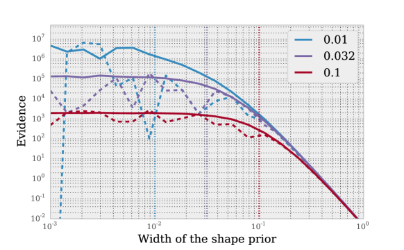
Figure 9.— Bayesian evidence of the shear posterior as a function of the assumed width in the galaxy shape prior in units of the galaxy intensity second moments. The different colors show different assumed values for the observational error (in units of the observed moments). The vertical lines denote the same 3 observational error values to offer a comparison with the peak locations in the colored lines. In all cases, the evidence reaches a maximum for values of the shape prior width (e.g., $\sqrt{\Sigma_{Q,{\rm prior}}}$) that is within a few times the observational error, with little information gained as the shape prior width decreases below the observational error. The solid lines assume no bias in the mean of the shape prior. The dashed lines show the evidence after marginalizing over the bias in the mean of the shape prior, with a Gaussian hyper-prior of width 0.07.

The evidence increases with decreasing shape prior width until the prior is of similar width to the observational errors in the galaxy moments (denoted by the vertical lines in Figure 9. This is a qualitative result that can be understood with intuition, but Fig. 9 now quantifies the information lost when the shape prior is a specific size relative to the observational errors and the observed moments.

We can also explore the requirements on specification of the mean of the shape prior by marginalizing over $\mu_{Q}$ in Equation F20 with a Gaussian hyperprior on $\mu_{Q}$ with mean equal to the true value (again denoted $\mu_{Q}$ in a convenient mangling of notation). The $\mu_{Q}$ marginalized results are shown by the dashed lines in Figure 9. We assume a shape prior mean hyperprior width of $0.07$ to marginalize over $\mu_{Q}$ (i.e., the mean of the prior on the moments is known to within $7\%$ of the moment values). In this case, the evidence assuming an observational error of 0.01 (blue dashed line) is similar to that assuming an observational error of 0.03 (purple dashed line). So, we might tolerate an unknown bias in the shape prior mean of up to 7% as long as the observational errors on the moments are $\sim 3$ times smaller than we would require if the shape prior mean were known perfectly.

While this numerical example is contrived, it illustrates the difficulty in constructing a scenario in which prior knowledge of the moments is not important.

References

- Antoniak (1974) Antoniak, C. E. 1974, The Annals of Statistics, 2, 1152
- Bard et al. (in prep.) Bard, D., Lang, D., Meyers, J., Marshall, P. J., Schneider, M. D., Boutigny, D., Dawson, W. A., & Hogg, D. W. in prep., in prep.
- Bartelmann & Schneider (2001) Bartelmann, M. & Schneider, P. 2001, Phys. Rep., 340, 291
- Bernstein (2010) Bernstein, G. M. 2010, MNRAS, 406, 2793