The Bethe Roots of Regge Cuts in
Strongly Coupled $\mathbf{{\cal{N}}=4}$ SYM Theory

Abstract

We describe a general algorithm for the computation of the remainder function for $n$-gluon scattering in multi-Regge kinematics for strongly coupled planar $\mathcal{N}=4$ super Yang-Mills theory. This regime is accessible through the infrared physics of an auxiliary quantum integrable system describing strings in AdS${}_{5}\times$S⁵. Explicit formulas are presented for $n=6$ and $n=7$ external gluons. Our results are consistent with expectations from perturbative gauge theory. This paper comprises the technical details for the results announced in Bartels:2014ppa .

1 Introduction

One of the major goals of modern theoretical physics is to construct the exact S-matrix of a four-dimensional interacting quantum field theory. It is believed that $\mathcal{N}=4$ super Yang-Mills (SYM) theory provides the simplest example for which this task may be achieved, at least in the planar limit. The first conjectured expression for gluon scattering amplitudes in this theory, known as the Bern-Dixon-Smirnov (BDS) formula Bern:2005iz , was shown to be incomplete for $n\geq 6$ external gluons beyond one-loop order Alday:2007he ; Bartels:2008ce ; Bartels:2008sc . The corrections to the BDS formula are captured by the so-called remainder function. For the maximally helicity violating (MHV) configuration the remainder function is known up to four loops Goncharov:2010jf ; Dixon:2013eka ; Dixon:2014voa for six gluons and up to two loops CaronHuot:2011ky ; Golden:2014xqf for seven gluons.

While the construction of the leading loop corrections to the BDS formula is a remarkable achievement which is based on beautiful and non-trivial mathematical concepts, these expressions are still a long way from an all-loop result (although first all-loop proposals have started to emerge recently Basso:2013vsa ; Basso:2013aha ; Basso:2014koa ; Basso:2014nra ). On the other hand, all-loop expressions do exist for the anomalous dimensions of local operators in $\mathcal{N}=4$ super Yang-Mills theory Beisert:2010jr ; Gromov:2013pga ; Gromov:2014caa . In that case, the initial progress from perturbative field theory computations Minahan:2002ve ; Beisert:2003tq ; Beisert:2003jj was soon complemented by string theoretic calculations Kazakov:2004qf which capture the behavior at strong coupling via the AdS/CFT correspondence Maldacena:1997re ; Witten:1998qj ; Gubser:1998bc . It were these investigations at strong coupling, such as Arutyunov:2004vx ; Beisert:2005cw ; Hernandez:2006tk ; Freyhult:2006vr ; Beisert:2006ib , that brought the breakthrough and paved the way for the first all-loop expressions of anomalous dimensions Beisert:2006ez .

Given the way things developed for the anomalous dimensions it seems worthwhile to invest more effort into the study of scattering amplitudes in strongly coupled $\mathcal{N}=4$ super Yang-Mills theory. All computations in this regime are based on the work of Alday and Maldacena Alday:2007hr who propose that scattering amplitudes in strongly coupled $\mathcal{N}=4$ super Yang-Mills theory are given by the area of a minimal surface in AdS₅ whose boundary is fixed to a piecewise light-like Wilson loop on the boundary of AdS₅. In a series of papers Alday:2009yn ; Alday:2009dv ; Alday:2010vh it is shown that this minimal area problem can be reformulated through a set of coupled non-linear integral equations, the so-called Y-system. These take a form which is familiar from the theory of one-dimensional quantum integrable models. They describe a system of excitations with certain masses and chemical potentials which live on a circle and which interact through an integrable $2\mapsto 2$ scattering. The interaction is engineered in such a way that the free energy of this system exactly reproduces the area of the minimal surface and thereby elegantly computes the amplitude.

In general, scattering amplitudes of four-dimensional quantum field theories are complicated functions of the kinematical invariants and the coupling constants. While the ultimate goal is to determine the full dependence on all of these variables, it might pay off to consider special kinematical limits at first. There are several choices which are being considered. These include, for example, two-dimensional kinematics Heslop:2010kq ; Goddard:2012cx ; Torres:2013vba ; Toledo:2014koa , the limit in which the boundary polygon becomes regular Alday:2010vh ; Hatsuda:2010vr ; Hatsuda:2011ke ; Hatsuda:2011jn ; Hatsuda:2012pb or the OPE limit of Alday:2010ku ; Gaiotto:2010fk ; Gaiotto:2011dt ; Sever:2011da ; Sever:2012qp ; Basso:2013vsa ; Basso:2013aha ; Basso:2014koa ; Basso:2014jfa . In this work we shall study a well-known kinematical limit that has a long history in gauge theory, the multi-Regge limit.

The multi-Regge limit has received much attention for two important reasons. On the one hand, it describes real scattering events at high energies which are observed at particle colliders. On the other hand, investigations in QCD revealed a second remarkable feature: It turns out that in the multi-Regge limit the quantities governing the scattering amplitude are controlled by the spectrum of an integrable spin chain Lipatov:1993yb ; Faddeev:1994zg . For $\mathcal{N}=4$ super Yang-Mills theory, these quantities are by now known to third order in perturbation theory Bartels:2008ce ; Bartels:2008sc ; Lipatov:2010ad ; Fadin:2011we ; Dixon:2012yy ; Dixon:2014voa and for the six-gluon case an all-loop conjecture was recently put forward in Basso:2014pla . Therefore, the situation somewhat mirrors the early development in the case of anomalous dimensions where the first few orders in perturbation theory were also controlled with the help of integrability.

Given this state of affairs it seems very natural to ask what the multi-Regge limit corresponds to on the strong coupling side. In Bartels:2010ej ; Bartels:2012gq we show that the multi-Regge limit of gauge theory corresponds to the infrared, or low temperature, limit of the Y-system. In such a low temperature limit, one can neglect the integral terms in the non-linear integral equations. What remains is a system of algebraic Bethe Ansatz equations which can be solved quite easily. The aim of this work is to explain these Bethe Ansatz equations and to explain how to construct the remainder functions from solutions of these equations. In order to illustrate the general algorithm we will then calculate the remainder function in multi-Regge kinematics for six and seven gluons. Our results are in agreement with features that are expected from the perturbative evaluation in the leading logarithmic approximation.

2 Multi-Regge kinematics

The aim of this section is to introduce the relevant kinematic invariants and to discuss their behavior in the multi-Regge limit. As is well known, the $n$-gluon remainder function depends on $3n-15$ cross ratios. For our discussion of $2\to n-2$ production amplitudes, we shall need a particular set of such cross ratios. This is discussed in the first subsection. We then turn to the multi-Regge limit and describe how our basis of cross ratios behaves as we go to high energies. The multi-Regge limit is described by the neighborhood of a particular point in the space of cross ratios. In order to exhibit interesting multi-Regge behavior, we must take the limit in various regions. These are discussed in the third subsection.

2.1 Kinematic variables

A scattering process of $n$ massless gluons is parametrized by kinematic invariants which can be built from products $p_{i}\cdot p_{j}$. After taking the on-shell conditions $p_{i}^{2}=0$ and momentum conservation into account, we count $D_{n}=\frac{1}{2}(n-1)(n-2)-1$ such product invariants. But these are not all independent. In fact, they are still subject to Gram determinant relations. There are $g_{n}=\frac{1}{2}(n-4)(n-5)$ such relations which arise from the fact that at most four vectors can be linearly independent in four dimensions and are obtained from the various vanishing $5\times 5$ subdeterminants of the $(n-1)\times(n-1)$ matrix $P_{ij}=(p_{i}\cdot p_{j})$, for details see appendix A. This leaves us with $D_{n}-g_{n}=3n-10$ independent Mandelstam invariants which parametrize our scattering problem.

In order to describe the multi-Regge limit of a $2\to n-2$ production amplitude, we introduce the standard Mandelstam invariants,

$$s_{i,\,j} =(p_{i}+\cdots+p_{j})^{2},\quad i=3,\dots,n-1,\,j=i+1,\dots,n,$$ (1)

$$t_{i} =(p_{2}+\cdots+p_{i+2})^{2},\quad i=1,\dots,n-3,$$

where we choose all momenta to be outgoing, as shown in figure 1.

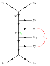
Figure 1: Graphical representation of the choice of Mandelstam variables as defined in Eq.  (1).

Note that there are $n-3$ $t$-like variables $t_{i}$ and $\frac{1}{2}(n-3)(n-2)$ $s$-like invariants. The latter include all subenergies, starting from the variables $s_{i}=s_{i+2,i+3}$ with $i=1,\dots,n-3$ for pairs of outgoing particles up to the total energy $s=s_{3,n}$ of the process. The overall number of these variables is $(n-3)+\frac{1}{2}(n-3)(n-2)=D_{n}$. One possible choice of independent kinematic invariants would include the $2n-6$ variables $t_{i}$ and $s_{i}$ along with $n-4$ variables $\eta_{a}$ which are defined by

$$\eta_{a}:=\frac{s_{a}s_{a+1}}{s_{a+2,a+4}},\quad a=1,\dots,n-4.$$ (2)

These are directly related to the subenergies $s_{a+2,a+4}$ for three outgoing particles. All higher subenergies are then obtained from the $t_{i},s_{i}$ and $\eta_{a}$ through the Gram determinant relations we described above.

Because of the dual conformal symmetry of $\mathcal{N}=4$ super Yang-Mills theory, the remainder function depends on fewer parameters. To introduce the relevant variables, let us parametrize the momenta $p_{i}$ through the dual variables $p_{i}=:x_{i-1}-x_{i}$, with $x_{i+n}=x_{i}$. The $x_{i}$ are position variables for the cusps of a light-like Wilson loop describing our momentum configuration. Along with the $x_{i}$ we also introduce $x_{i,j}^{2}=(x_{i}-x_{j})^{2}$ for $i,j=1,\dots,n$, which are just the Mandelstam invariants introduced before. Note that $x_{i,i}^{2}=x_{i,i+1}^{2}=0$, since we are considering a light-like Wilson loop. Hence, the $x_{i,j}^{2}$ provide $D_{n}=\frac{1}{2}n(n-3)$ Mandelstam invariants which we may arrange in an $n\times n$ matrix $X_{ij}:=(x_{i,j}^{2})$. The $x_{i,j}^{2}$ possess a rather simple relation with the Mandelstam invariants we described above. In the case of $n=7$ external gluons, for example, one has

$$X=\begin{bmatrix}\ 0\ &\ 0\ &\ x_{1,3}^{2}\ &\ x_{1,4}^{2}\ &\ x_{1,5}^{2}\ &\ x_{1,6}^{2}\ &\ 0\ \\[2.84526pt] 0&0&0&x_{2,4}^{2}&x_{2,5}^{2}&x_{2,6}^{2}&x_{2,7}^{2}\\[2.84526pt] x_{1,3}^{2}&0&0&0&x_{3,5}^{2}&x_{3,6}^{2}&x_{3,7}^{2}\\[2.84526pt] x_{1,4}^{2}&x_{2,4}^{2}&0&0&0&x_{4,6}^{2}&x_{4,7}^{2}\\[2.84526pt] x_{1,5}^{2}&x_{2,5}^{2}&x_{3,5}^{2}&0&0&0&x_{5,7}^{2}\\[2.84526pt] \phantom{mm}&\ &\ &\ &0&0&0\\[2.84526pt] \ &\ &\ &\ &\ &0&0\end{bmatrix}\ =\ \begin{bmatrix}\ 0\ &\ 0\ &\ \ t_{1}\ &\ t_{2}\ &\ t_{3}\ &\ t_{4}\ &\ 0\ \\[2.84526pt] 0&0&0&\ s_{1}\ &\ s_{3,5}\ &\ s_{3,6}\ &\ s\ \\[2.84526pt] t_{1}&0&0&0&s_{2}&s_{4,6}&s_{4,7}\\[2.84526pt] t_{2}&s_{1}&0&0&0&s_{3}&s_{5,7}\\[2.84526pt] t_{3}&s_{3,4}&s_{2}&0&0&0&s_{4}\\[2.84526pt] \phantom{mm}&\ &\ &\ &0&0&0\\[2.84526pt] \ &\ &\ &\ &\ &0&0\end{bmatrix},$$ (3)

where the entries not shown can be obtained by the symmetry $X_{ij}=X_{ji}$. For other numbers $n$ of external gluons, the relations take a similar form, with $t$-like variables in the first row and all the $s$-like variables filling a triangle in row $2$ to $n-2$.

From these Mandelstam invariants we can easily construct $D_{n}-n$ dual conformal invariant quantities

$$U_{ij}=\frac{x^{2}_{i,j+1}x^{2}_{i+1,j}}{x^{2}_{i,j}x^{2}_{i+1,j+1}},$$ (4)

which are called cross ratios. Once again, these are not all independent. Additional relations are obtained from the $c_{n}=\frac{1}{2}(n-5)(n-6)$ conformal Gram relations which state that all $7\times 7$ subdeterminants of the matrix $X$ must vanish (cf. appendix A). They leave us with $D_{n}-n-c_{n}=3n-15$ independent cross ratios.

As in our discussion of independent Mandelstam invariants, it is useful to fix an independent set of cross ratios which is adapted to the multi-Regge limit of a $2\to n-2$ production amplitude. In Bartels:2012gq we suggest to use

$$u_{1\sigma} =U_{\sigma+1,\sigma+4}=\frac{x^{2}_{\sigma+1,\sigma+5}x^{2}_{\sigma+2,\sigma+4}}{x^{2}_{\sigma+2,\sigma+5}x^{2}_{\sigma+1,\sigma+4}},$$ (5)

$$u_{2\sigma} =U_{\sigma+2,n}=\frac{x^{2}_{\sigma+3,n}x^{2}_{1,\sigma+2}}{x^{2}_{\sigma+2,n}x^{2}_{1,\sigma+3}},$$ (6)

$$u_{3\sigma} =U_{1,\sigma+3}=\frac{x^{2}_{2,\sigma+3}x^{2}_{1,\sigma+4}}{x^{2}_{2,\sigma+4}x^{2}_{1,\sigma+3}},$$ (7)

where $\sigma=1,\dots,n-5$. All other cross ratios, and in particular those defined in Eq. (4), may be reconstructed from the $u_{a\sigma}$ by solving the conformal Gram determinant relations (see appendix A for the unique Gram relation in the $7$-gluon case). A convenient graphical representation of the cross ratios Eqs. (5)-(7) is shown in figure 2.

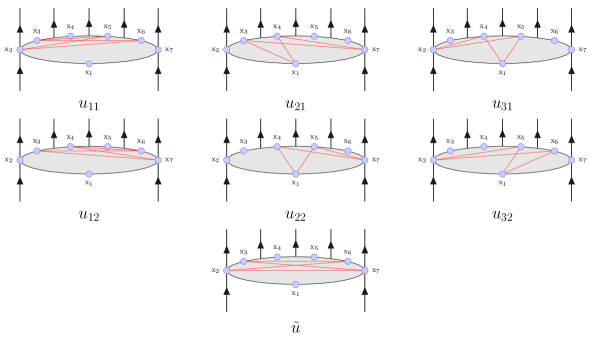
Figure 2: Graphical representation of the cross ratios for the $7$-gluon amplitude. The cross ratios $u_{as}$ are chosen to be independent (cf. Eqs. (5)-(7)), while $\tilde{u}$ depends on those cross ratios through a conformal Gram relation.

A symmetry we will use later is target-projectile symmetry, which, as the name suggests, reflects the fact that the amplitude should remain invariant when the two incoming particles $p_{1}$, $p_{2}$ are swapped. In terms of the graphical representation of the cross ratios in figure 2, target-projectile symmetry simply amounts to a reflection on the central vertical axis of each blob. From this, it is easy to deduce that applying target-projectile symmetry amounts to the following exchange of cross ratios

$$u_{1\sigma}\ \leftrightarrow\ u_{1(n-4-\sigma)},\quad u_{2\sigma}\ \leftrightarrow u_{3(n-4-\sigma)}\ \ .$$ (8)

2.2 The multi-Regge regime

By definition, the multi-Regge regime is reached when we impose a strong ordering of the rapidities of the outgoing particles $p_{3},\dots,p_{n}$ while keeping their transverse momenta of the same order. For the Mandelstam variables this translates into all $s$-like variables becoming large with $t$-like variables fixed. More precisely, we get a hierarchy

$$s=s_{3,n}\gg s_{3,n-1},s_{4,n}\gg\dots\gg s_{i,i+2}\gg s_{i}\gg-t_{i}\ .$$ (9)

In terms of the matrix $X_{ij}$ introduced in Eq.  (3) this means that the $s$-like variables become larger as we go to the upper right corner. This scaling of kinematic invariants is discussed in more detail in Bartels:2012gq . In the limiting regime one finds that

$$x_{ij}^{2}=s_{i+1,j}\sim s_{i-1}\cdots s_{j-3}\ .$$ (10)

As we can easily infer from Eq.  (10) and our definition of the independent cross ratios (5)-(7), the limiting behavior of the $u_{a\sigma}$ is therefore given by

$$u_{2\sigma}\sim\frac{1}{s_{\sigma+1}},\quad u_{3\sigma}\sim\frac{1}{s_{\sigma+1}},\quad 1-u_{1\sigma}\sim\frac{1}{s_{\sigma+1}}\ .$$ (11)

Hence, the approach to the multi-Regge limit is characterized by the finite, reduced cross ratios

$$\tilde{u}_{2\sigma}:=\frac{u_{2\sigma}}{1-u_{1\sigma}}=:\frac{1}{|1+w_{\sigma}|^{2}},\quad\tilde{u}_{3\sigma}:=\frac{u_{3\sigma}}{1-u_{1\sigma}}=:\frac{|w_{\sigma}|^{2}}{|1+w_{\sigma}|^{2}},$$ (12)

where we introduced the complex quantities $w_{\sigma}$ as in Lipatov:2010ad . Let us note that the other cross ratios $U_{ij}$ with $i>1$ and $j<n$ possess the limiting behavior

$$U_{ij}-1\sim s_{i}^{-1}\cdots s_{j-3}^{-1}\ \ .$$ (13)

For example, in the case of $n=7$ we can easily see that $\tilde{u}:=U_{26}$ approaches $1$ in the multi-Regge limit, as it must in order to satisfy the conformal Gram relation we spell out in appendix A. In fact, inserting $u_{1\sigma}=1$ and $u_{2\sigma}=u_{3\sigma}=0$ into Eq.  (140) leads to the Gram relation $(\tilde{u}-1)^{2}=0$.

2.3 Multi-Regge regions

As we shall discuss below, it is very important to evaluate the multi-Regge limit in different kinematical regions. In fact, in the so-called Euclidean region where all kinematic invariants are negative, the multi-Regge limit of the remainder function vanishes. If this was the only admissible regime, the multi-Regge limit would be incapable of distinguishing between the BDS Ansatz and the true scattering amplitude. Fortunately, we have more freedom in taking the multi-Regge limit.

In the Euclidean region, the energy components $p_{i}^{0}$ of the four-momenta $p_{i}$ of the produced particles are taken to be positive. In other words, all the $p_{i}$ take values in the forward light cone. But we can admit different choices for the sign of $p_{i}^{0}$. These characterize $2^{n-4}$ admissible kinematical regions. Let us define an associated map

$$\varrho_{i}=\mathit{sgn}(p_{i}^{0})\in\{\pm 1\},$$ (14)

by which we parametrize the region $(\varrho_{4}\cdots\varrho_{n-1})$. It is possible to characterize the regions through the behavior of Mandelstam invariants and cross ratios. For the Mandelstam invariants, the $t$-like variables remain negative while $s$-like variables may change sign. Because of Eq.  (10), the approach to the multi-Regge limit is characterized by the following behavior

$$\varrho_{i}\varrho_{j}\ s_{i,j}\geq 0\,$$ (15)

with $\varrho_{3}=\varrho_{n}=1$. Furthermore, note that the sign of the $s$-like variables is uniquely characterized by the signs of the two-particle invariants $s_{i}$, using the multi-Regge behavior (10).

Let us now pass to the cross ratios. In the Euclidean regime, all cross ratios are positive since they involve an even number of $t$-like invariants. But once we pass to other regions, the cross ratios $u_{2\sigma}$ and $u_{3\sigma}$ may change signs according to the rules

$$\varrho_{\sigma+3}\varrho_{\sigma+4}\ u_{2\sigma}\geq 0,\quad\varrho_{\sigma+3}\varrho_{\sigma+4}\ u_{3\sigma}\geq 0,$$ (16)

where $\sigma=1,\dots,n-5$. Note that the signs of these cross ratios are not sufficient to specify the regime as they leave one sign undetermined.

We can pass from one multi-Regge region to another by analytic continuation in the kinematic invariants. In going from the Euclidean region with all the $u_{a\sigma}$ positive to another region that is characterized by factors $\varrho_{i}$, we shall use a curve for which the cross ratios $U_{ij}$ possess non-vanishing winding number $n_{ij}$ around $U_{ij}=0$. This winding number is related to the parameters $\varrho_{i}$ through

$$n_{ij}=\frac{1}{4}(\varrho_{i+1}-\varrho_{i+2})(\varrho_{j}-\varrho_{j+1}).$$ (17)

Winding number $n=1$ means that we encircle the origin of the U-plane in clockwise direction, while $n=-1$ corresponds to a counter-clockwise rotation. The formula for $n_{ij}$ can be used for all $i,j=1,\dots,n$ if we extend the definition of $\varrho_{i}$ such that $\varrho_{1}=\varrho_{2}=\varrho_{n+1}=\varrho_{n+2}=2$. For the small cross ratios $u_{2\sigma}=U_{\sigma+2,n}$ and $u_{3\sigma}=U_{1,\sigma+3}$ the winding number $n_{ij}$ is given by $\pm\frac{1}{2}$. The winding numbers for all other cross rations are integer valued, i.e. these cross ratios perform full rather than half rotations.

The precise curve along which we perform the continuation must be constructed such that

• all winding numbers assume the prescribed values (17) and

• all conformal Gram determinant relations are respected.

For the cross ratios $u_{2\sigma}$ and $u_{3\sigma}$ we propose the following simple behavior

$$u_{2\sigma}(\varphi)=e^{\frac{i}{2}(\varrho_{\sigma+3}-\varrho_{\sigma+4})\varphi}\ u_{2\sigma},\quad u_{3\sigma}(\varphi)=e^{\frac{i}{2}(\varrho_{\sigma+4}-\varrho_{\sigma+3})\varphi}\ u_{3\sigma},$$ (18)

where $\varphi\in[0,\pi]$ parametrizes the curve along which we continue. This is the simplest behavior that is consistent with our formula (17) and it changes the signs of the cross ratios $u_{2\sigma}$ and $u_{3\sigma}$ such that we end up in the desired region, see Eq. (16). For all other cross ratios the dependence on $\varphi$ is more complicated, at least in general. The simplest curves that possess the correct winding numbers are, of course, circles. However, as we shall see in some examples below, having all the cross ratios move along circles is rarely ever consistent with the Gram relations.

Let us consider some specific examples. In the case of $n=6$ we have four multi-Regge regions including the Euclidean one. Hence there are three non-trivial paths connecting the Euclidean region to the three others. These are given by

$$P_{6,+-}:\, u_{11}(\varphi)=u_{11},\quad u_{21}(\varphi)=e^{i\varphi}u_{21},\quad u_{31}(\varphi)=e^{-i\varphi}u_{31}$$ (19)

$$P_{6,-+}:\, u_{11}(\varphi)=u_{11},\quad u_{21}(\varphi)=e^{-i\varphi}u_{21},\quad u_{31}(\varphi)=e^{i\varphi}u_{31}$$ (20)

$$P_{6,--}:\, u_{11}(\varphi)=e^{-2i\varphi}u_{11},\quad u_{21}(\varphi)=u_{21},\quad u_{31}(\varphi)=u_{31},\$$ (21)

where the subscript $\pm$ indicates the signs of the energies we choose for the produced particles. Since there are no further cross ratios and no conformal Gram relations to satisfy, it is obvious that our three curves possess all the desired properties.

If we choose $n=7$ there are eight multi-Regge regions. One is the Euclidean region, three others correspond to a single change of signs. For the latter, none of the integer winding numbers $n_{ij}$ with $i>1$ and $j<n$ is actually non-zero. Such curves will turn out to lead to regions with trivial Regge limit, both at weak and strong coupling. It therefore suffices to discuss the remaining four curves. Extending our general prescription in Eq. (18), the first three of them are given by

$$P_{7,+--}:\, u_{11}(\varphi)=u_{11},\quad u_{21}(\varphi)=e^{i\varphi}u_{21},\quad u_{31}(\varphi)=e^{-i\varphi}u_{31},$$ (22)

$$u_{12}(\varphi)=e^{-2i\varphi}u_{12},\quad u_{22}(\varphi)=u_{22},\quad u_{32}(\varphi)=u_{32},\quad \tilde{u}(\varphi)=\tilde{u}$$

$$P_{7,-+-}:\, u_{11}(\varphi)=e^{2i\varphi}u_{11},\quad u_{21}(\varphi)=e^{-i\varphi}u_{21},\quad u_{31}(\varphi)=e^{i\varphi}u_{31},$$ (23)

$$u_{12}(\varphi)=e^{2i\varphi}u_{12},\quad u_{22}(\varphi)=e^{i\varphi}u_{22},\quad u_{32}(\varphi)=e^{-i\varphi}u_{32},\quad \tilde{u}(\varphi)=e^{-2i\varphi}\tilde{u}$$

$$P_{7,--+}:\, u_{11}(\varphi)=e^{-2i\varphi}u_{11},\quad u_{21}(\varphi)=u_{21},\quad u_{31}(\varphi)=u_{31},$$ (24)

$$u_{12}(\varphi)=u_{12},\quad u_{22}(\varphi)=e^{-i\varphi}u_{22},\quad u_{32}(\varphi)=e^{i\varphi}u_{32},\quad \tilde{u}(\varphi)=\tilde{u}\ .$$

It should be noted that the paths spelled out above satisfy the Gram relation only in the multi-Regge limit, i.e. when Eq.(11) holds. This, however, is satisfied for all cases studied in this paper. In order to reach the forth region, in which all $\varrho_{i}=-1$, the conformal Gram relations force us to consider a more complicated curve. It is still easy to give an explicit expression in the limit where $u_{2\sigma}=u_{3\sigma}=0$,

$$P_{7,---}:\, u_{11}(\varphi)=e^{2i\varphi}\left(1-\sqrt{1-e^{-2i\varphi}}\right)u_{11},\quad u_{21}(\varphi)=u_{21},\quad u_{31}(\varphi)=u_{31},$$ (25)

$$u_{12}(\varphi)=e^{2i\varphi}\left(1-\sqrt{1-e^{-2i\varphi}}\right)u_{12},\quad u_{22}(\varphi)=u_{22},\quad u_{32}(\varphi)=u_{32},\quad \tilde{u}(\varphi)=e^{-2i\varphi}\tilde{u}.$$

In the multi-Regge limit, the parameters $u_{2\sigma}$, $u_{3\sigma}$ become small so that $P_{---}$ is a good approximation. This last path illustrates nicely that one cannot always analytically continue along circles. Just computing the winding numbers for this path, we find that the cross ratios $u_{a\sigma}$ we choose as independent variables have winding number zero, while the cross ratio $\tilde{u}$, which is given in terms of the independent cross ratios via the conformal Gram relation, has winding number $\tilde{n}=+1$. This is impossible to realize with $u_{1\sigma}(\varphi)=u_{1\sigma}$ constant because the conformal Gram relations would force $\tilde{u}$ to be constant, as well. Choosing the path for $\tilde{u}$ to run along a circle, as we did in our prescription for $P_{7,---}$, we can solve Eq.  (142) for $u_{11}$, $u_{12}$ while preserving the target-projectile symmetry along the entire path. This leads to the expressions we have prescribed. Note that the Gram determinant relation (142) has been derived with the additional assumption that $u_{2\sigma}=u_{3\sigma}=0$. Hence, our curve $P_{7,---}$ is only valid in the multi-Regge limit.

2.4 Weak coupling results

On the weak coupling side, soon after the BDS conjecture for the planar $n$-point scattering amplitude had been published, it became clear that for more than five external legs the BDS formula is incomplete. The missing pieces are encoded in the remainder functions, $R_{n}$, and in recent years intense work has been devoted to the calculation of these functions. The multi-Regge limit provides enormous help in determining $R_{n}$.

Starting point is the multi-Regge analysis of the $2\to 4$ scattering amplitude in the leading logarithmic approximation. In Bartels:2008ce ; Bartels:2008sc it is shown that the failure of the BDS formula is due to the existence of Regge cut contributions. More precisely, the perturbative analysis shows that the high-energy behavior of the $2\to 4$ scattering process is described by the exchange of Regge poles - the reggeizing gluon - and a Regge cut consisting of the exchange of two interacting reggeized gluons. In the planar approximation this cut is present only in specific kinematic regions which have been named Mandelstam regions. The BDS formula does not account for this Regge cut contribution. As shown in Bartels:2008ce , it contains the Regge poles, and the phase structure is correct in the Euclidean region (where all energies are negative) and in the physical region where all energies are positive. In the Mandelstam region where the Regge cut appears in the perturbative analysis, the BDS formula exhibits a phase which has been identified as the one-loop part of the Regge cut contribution. At the same time, in these kinematic regions the phase structure of the Regge pole contributions is not correctly reproduced by the BDS formula Lipatov:2010qf .

In fact, there is a close connection between the structure of Regge pole contribution and the existence of Regge cut contributions Bartels:2013jna . In the planar approximation, the Regge pole expression for the $2\to n-2$ amplitude has a simple factorizing form in only some kinematic regions, such as the Euclidean region or the region of positive energies. In contrast, just in those kinematic regions where the Regge cut contributions are present, the Regge pole expressions develop unphysical singularities which have to be canceled by the Regge cut singularities. The existence of Regge cuts, therefore, is required to provide a consistent (i.e. singularity-free and, in the case of $\mathcal{N}=4$ SYM, also conformally invariant) description of Regge poles.

The general analysis of the structure of the Regge pole contributions in $2\to n-2$ scattering amplitudes is presented in Bartels:2013jna . In particular, this analysis allows to find the analytic form of the Regge pole contributions for planar amplitudes in all kinematic regions, including the singular pieces which have to be canceled by the Regge cut contributions. Details are worked out for the cases $2\to 4$ and $2\to 5$ in Bartels:2013jna , and in Bartels:yyyy for the case $2\to 6$.

The calculation of the Regge cut contributions is based upon the calculation of energy discontinuities using unitarity integrals. In order to obtain energy discontinuities one needs the analytic representation of the scattering amplitudes in multi-Regge kinematics which, in agreement with the Steinmann relations, exhibits the dependence upon the energy variables, including the phases in the different kinematic regions. The authors of Bartels:xxxx outline a general strategy for the calculation of Regge cut contributions. These contain the singular terms which exactly cancel the singular terms of the Regge pole contributions: when pole and cuts are combined one finds a sum of infrared finite and conformally invariant pole and cut expressions. Explicit leading order result for the $2\to 5$ and $2\to 6$ cases are obtained in Bartels:xxxx and Bartels:yyyy , respectively.

Let us briefly summarize some of those results which are of special interest for the analysis described in this paper. To be complete we begin with the $2\to 4$ case. The Regge cut appears in the kinematic region $(--)$: this is the one which is studied in Bartels:2010ej and it is contained in the list (19) - (21). In terms of Mandelstam variables the energies have the following sign structure

$$s,s_{2}>0,\,s_{1},s_{3},s_{3,5},s_{4,6}<0\ .$$ (26)

Note that there is a second region, not mentioned in the above list, in which the cut appears: it is obtained by ‘twisting’ the $t_{2}$ channel. The other two regions, $(+-)$ and $(-+)$, do not contain the Regge cut contribution. The corresponding path of analytic continuation for the region $(--)$ is described in Eq. (21). It is possible to define other, more complicated paths which connect the same starting and final values of energies, but the path Eq. (21) appears to be the simplest one. The Regge cut amplitude which emerges after combination with the Regge pole contribution is derived in Bartels:2008sc and the full remainder function in this region is obtained in Bartels:xxxx :

$$\left[e^{R_{6}+i\delta_{6,--}}\right]_{--}=\cos\pi\omega_{ab}+i\delta_{6,--}+2if_{\omega_{2}}\ .$$ (27)

In terms of the cross ratios the cut amplitude $f_{\omega_{2}}$ has the form:

$$f_{\omega_{2}}=\frac{g^{2}N_{c}}{16\pi^{2}}\sum_{n}(-1)^{n}\left(\frac{w}{w^{*}}\right)^{\frac{n}{2}}\int\frac{d\nu}{2\pi i}\Phi_{\nu,n}^{*}\left[\left(-\sqrt{u_{2}u_{3}}\right)^{-\omega(\nu,n)}-1\right]\Phi_{\nu,n}|w|^{2i\nu},$$ (28)

where $w=w_{1}$ was introduced in Eq. (12). Here $\Phi_{\nu,n}$ denotes the impact factor and $\omega(\nu,n)$ is the eigenvalue function of the color octet BFKL Hamiltonian. These quantities are known up to next-to-leading order from direct field theory calculations Bartels:2008sc ; Lipatov:2010ad ; Fadin:2011we . Using the bootstrap program of Dixon:2013eka ; Dixon:2014voa , the BFKL eigenvalue and the impact factor can be determined up to NNLLA and N³LLA, respectively, and all-order expressions derived from the Wilson loop OPE are put forward in Basso:2014jfa .

In Lipatov:2009nt it is shown that the BFKL Hamiltonian is equivalent to the non-compact $SL(2,C)$ Heisenberg Hamiltonian for an open spin chain, with $\omega(\nu,n)$ being the eigenvalue function for the spin chain of length two.

Next we turn to the case $2\to 5$ Bartels:xxxx . Here, the weak-coupling analysis leads to three different Regge cut contributions composed of two reggeized gluons, two ‘short’ cuts in the $t_{2}$ and $t_{3}$ channels, respectively, and one ‘long cut’ extending over the $t_{2}$ and the $t_{3}$ channels. The different kinematic regions in which these cuts appear are listed in Eqs. (22)-(25), together with simple choices of paths of analytic continuation. The simplest cases are $(+--)$ and $(--+)$: they contain only the short cuts in the $t_{3}$ and the $t_{2}$ channels, respectively. In these regions the remainder function has the following form

$$\left[e^{R_{7}+i\delta_{7,+--}}\right]_{+--} =\cos\pi\omega_{bc}+i\delta_{7,+--}+2if_{\omega_{3}}$$ (29)

$$\left[e^{R_{7}+i\delta_{7,--+}}\right]_{--+} =\cos\pi\omega_{ab}+i\delta_{7,--+}+2if_{\omega_{2}}$$ (30)

The integral expressions for the Regge cut amplitudes $f_{\omega_{2}}$ and $f_{\omega_{3}}$ are easily obtained from Eq. (28) by substituting the cross ratios $u_{i}\to u_{i\sigma}$. For the remaining two regions also the long cut contributes. For $(---)$ and $(-+-)$ the remainder functions are given by

$$\left[e^{R_{7}+i\delta_{7,---}}\right]_{---} =\cos\pi\omega_{ac}+i\delta_{7,---}+2if_{\omega_{2}\omega_{3}}$$ (31)

$$\left[e^{R_{7}+i\delta_{7,-+-}}\right]_{-+-} =e^{i\pi\omega_{ba}}e^{i\pi\omega_{bc}}+i\delta_{7,-+-}+2i(f_{\omega_{2}\omega_{3}}-e^{i\pi\omega_{bc}}f_{\omega_{2}}-e^{i\pi\omega_{ba}}f_{\omega_{3}}).$$ (32)

The integral for the long cut reads

$$f_{\omega_{2}\omega_{3}}= \frac{a}{2}\sum_{n_{1},n_{2}}(-1)^{n_{1}+n_{2}}\left(\frac{w_{1}}{w_{1}^{*}}\right)^{n_{1}}\left(\frac{w_{2}}{w_{2}^{*}}\right)^{n_{2}}\int\frac{d\nu_{1}d\nu_{2}}{(2\pi)^{2}}\Phi(\nu_{1},n_{1})^{*}|w_{1}|^{2i\nu_{1}}\left(-\sqrt{u_{21}u_{31}}\right)^{-\omega(\nu_{1},n_{1})}$$ (33)

$$C(\nu_{1},\nu_{2},n_{1},n_{2})\left(-\sqrt{u_{22}u_{32}}\right)^{-\omega(\nu_{2},n_{2})}|w_{2}|^{2i\nu_{2}}\Phi(\nu_{2},n_{2})|_{\text{sub}}.$$

Here the impact factor $\Phi(\nu,n)$ is the same as in Eq. (28), and $C(\nu_{1},\nu_{2},n_{1},n_{2})$ stands for the central production vertex. The latter is known in leading order Bartels:2011ge . The subscript $|_{sub}$ indicates that we have subtracted the one-loop contribution. In Bartels:xxxx a few more kinematic regions with Regge cut contributions are listed; they will not be mentioned here.

It is important to note that in leading order the integral representation is real-valued up to the phase factors $e^{-i\pi\omega(\nu_{i},n_{i})}$. Beyond leading order this will no longer be the case. As explained in Bartels:xxxx , one can still write the Regge cut amplitude in the form of Eq. (33), but with a complex-valued expression for the production vertex $C$. Alternatively, the amplitude breaks into two pieces with different phase factors.

Before we turn to the strong coupling regime let us make a final remark on the weak coupling results summarized in this section. Comparing the results for the $2\to 4$ scattering amplitude with those of the $2\to 5$ case we would like to stress the close connections. Obviously the short Regge cuts in the $2\to 5$ case have the same functional form as the $2\to 4$ cut contribution (with suitable replacements of the cross ratios), i.e. the same impact factor and eigenvalue function $\omega(\nu,n)$. Also the expression for the long cut contains - apart from the new production vertex - the same building blocks.

New elements appear in the $2\to 6$ scattering amplitude: in the region $(-++-)$ one finds a Regge cut consisting of three reggeized gluons. Apart from a new impact factor, a new eigenvalue function $\omega_{3}(\nu_{1},n_{1};\nu_{2},n_{2})$ appears which belongs to a spin chain of length three and can be parametrized by two sets of conformal quantum numbers. In leading order this eigenvalue function can be written as a sum of the two functions $\omega(\nu_{1},n_{1})$ and $\omega(\nu_{2},n_{2})$ Lipatov:2009nt ; Derkachov:2014gya . Whether this simple additivity remains valid also beyond leading order is presently not known.

3 Scattering amplitude at strong coupling

In this section we shall outline the general algorithm for the calculation of the remainder function of strongly coupled $\mathcal{N}=4$ SYM in the multi-Regge limit. All the key elements of our description are applicable for any number $n$ of external gluons. There are a few formulas that we shall only spell out for $n=7$ because their precise form for other values of $n$ is irrelevant both for the presentation of the general algorithm and for the example we shall work out in the next section. After reviewing the form of the scattering amplitude and its relation with a special set of thermodynamic Bethe Ansatz equations, we will discuss how to perform the multi-Regge limit. In particular we shall show that the multi-Regge limit is a particular large mass limit in the underlying thermodynamic Bethe Ansatz. In such a large mass limit, the thermodynamic Bethe Ansatz equations get replaced by a much simpler set of algebraic Bethe Ansatz equations. The latter will be described explicitly in the third subsection. We conclude the section by illustrating the general algorithm through the simplest example, namely the case of $n=6$ gluons, and explain how to evaluate the various contributions to the remainder function in the multi-Regge limit. For the least trivial contribution to the remainder function this will lead to a set of Bethe Ansatz equations. Special solutions of these Bethe Ansatz equations are associated with the various kinematical regions discussed above.

3.1 Amplitude and thermodynamic Bethe Ansatz

The problem of calculating strong coupling scattering amplitudes to leading order was solved in a series of papers Alday:2007hr ; Alday:2009yn ; Alday:2009dv ; Alday:2010vh , the solution of which we will briefly review here.

It turns out that the leading order of the $n$-gluon scattering amplitude can be written as

$$\mathcal{A}\ \sim\ e^{-\frac{\sqrt{\lambda}}{2\pi}\mathrm{A}}=e^{-\frac{\sqrt{\lambda}}{2\pi}\mathrm{A}_{\text{BDS}}+R}$$ (34)

where the quantity $\mathrm{A}$ consists of several different terms to be discussed one by one,

$$\mathrm{A}=\mathrm{A}_{\mathrm{div}}+\mathrm{A}_{\mathrm{free}}+\mathrm{A}_{\mathrm{BDS-like}}+\mathrm{A}_{\mathrm{per}}\ .$$ (35)

Let us discuss the four different contributions in the order of their appearance. To begin with, $\mathrm{A}_{\mathrm{div}}$ encodes the infrared divergences of the amplitude and it reads

$$\mathrm{A}_{\mathrm{div}}\ =\ \frac{1}{8}\sum\limits_{i}\log^{2}\left(\varepsilon^{2}x^{2}_{i,i+2}\right),$$ (36)

where $\varepsilon$ is a radial cutoff for AdS₅. The next term $\mathrm{A}_{\mathrm{free}}$ is the most interesting and least trivial one. As we anticipated in the introduction, it is constructed from a one-dimensional auxiliary quantum integrable system. For the $n$-gluon amplitude, it is defined in terms of $3n-15$ functions, ${\rm Y}_{a,s}(\theta)$, where $a=1,2,3$ and $s=1,\dots,n-5$. These functions are determined by a set of non-linear integral equations, called the Y-system equations,

$$\mathrm{log}{\rm Y}_{1,s} =-m_{s}\cosh\theta-C_{s}-\frac{1}{2}K_{2}\star\beta_{s}-K_{1}\star\alpha_{s}-\frac{1}{2}K_{3}\star\gamma_{s},$$ (37)

$$\mathrm{log}{\rm Y}_{2,s} =-m_{s}\sqrt{2}\cosh\theta-K_{2}\star\alpha_{s}-K_{1}\star\beta_{s},$$ (38)

$$\mathrm{log}{\rm Y}_{3,s} =-m_{s}\cosh\theta+C_{s}-\frac{1}{2}K_{2}\star\beta_{s}-K_{1}\star\alpha_{s}+\frac{1}{2}K_{3}\star\gamma_{s},$$ (39)

where $m_{s}$ and $C_{s}$ are parameters that one can think of as mass parameters and chemical potentials of excitations in the one-dimensional auxiliary quantum system. The objects $\alpha_{s}$, $\beta_{s}$, $\gamma_{s}$ that appear on the right hand side are defined in terms of the functions ${\rm Y}_{a,s}$ as

$$\alpha_{s} =\mathrm{log}\frac{(1+{\rm Y}_{1,s})(1+{\rm Y}_{3,s})}{(1+{\rm Y}_{2,s-1})(1+{\rm Y}_{2,s+1})},$$ (40)

$$\beta_{s} =\mathrm{log}\frac{(1+{\rm Y}_{2,s})^{2}}{(1+{\rm Y}_{1,s-1})(1+{\rm Y}_{1,s+1})(1+{\rm Y}_{3,s-1})(1+{\rm Y}_{3,s+1})},$$ (41)

$$\gamma_{s} =\mathrm{log}\frac{(1+{\rm Y}_{1,s-1})(1+{\rm Y}_{3,s+1})}{(1+{\rm Y}_{1,s+1})(1+{\rm Y}_{3,s-1})}.$$ (42)

In the Y-system these combinations of ${\rm Y}$-functions are convoluted with the following simple kernel functions

$$K_{1}=\frac{1}{2\pi}\frac{1}{\cosh\theta},\quad K_{2}=\frac{\sqrt{2}}{\pi}\frac{\cosh\theta}{\cosh 2\theta},\quad K_{3}=\frac{i}{\pi}\tanh 2\theta.$$ (43)

These kernel functions can be thought of as describing the (integrable) interaction between the excitations of the auxiliary quantum system. Let us also recall that the convolution product is defined as

$$(K\ast f)(\theta)\ =\ \int\limits_{-\infty}^{\infty}d\theta^{\prime}K(\theta-\theta^{\prime})f(\theta^{\prime})\ .$$ (44)

The spectral parameter $\theta$ in the Y-system equations is a complex variable. From the definition (43) of the kernel functions it is clear that for certain values of $\theta$, the kernels can become singular. Therefore, the form of the Y-system as presented in Eqs. (37)-(39) is only valid for $\left|\mathrm{Im}\,\theta\right|\leq\frac{\pi}{4}$. If we wish to evaluate the Y-system for larger imaginary parts of $\theta$, we have to pick up residues or use a powerful recursion relation for the Y-functions,

$$\mathrm{Y}_{a,s}^{\left[r\right]}=\frac{\left(1+\mathrm{Y}_{a,s+1}^{\left[r+1\right]}\right)\left(1+\mathrm{Y}_{4-a,s-1}^{\left[r+1\right]}\right)}{\mathrm{Y}_{4-a,s}^{\left[r+2\right]}\left(1+\frac{1}{\mathrm{Y}_{a+1,s}^{\left[r+1\right]}}\right)\left(1+\frac{1}{\mathrm{Y}_{a-1,s}^{\left[r+1\right]}}\right)},$$ (45)

where $\mathrm{Y}_{a,s}^{\left[r\right]}(\theta)={\rm Y}_{a,s}(\theta+ir\pi/4)$ denotes a shift in $\theta$ by a multiple of $i\frac{\pi}{4}$. When using the recursion relation, it should be noted that ${\rm Y}_{0,s}={\rm Y}_{4,s}=\infty$, as well as ${\rm Y}_{a,0}={\rm Y}_{a,n-4}=0$.
An additional modification of the Y-system equations has to be made when the parameters $m_{s}$ become complex, i.e. $m_{s}=|m_{s}|e^{i\phi_{s}}$. In this case, we have to substitute

$$m_{s}\rightarrow\left|m_{s}\right|,\quad{\rm Y}_{a,s}(\theta)\rightarrow\tilde{{\rm Y}}_{a,s}(\theta):={\rm Y}_{a,s}(\theta+i\phi_{s}),$$ (46)

$$K^{a,a^{\prime}}_{s,s^{\prime}}(\theta-\theta^{\prime})\rightarrow K^{a,a^{\prime}}_{s,s^{\prime}}(\theta-\theta^{\prime}+i(\phi_{s}-\phi_{s^{\prime}})),$$ (47)

in Eqs. (37)-(39), as is shown in Alday:2010vh . Once we solve the Y-system equations for the $\tilde{{\rm Y}}_{a,s}$, we can finally calculate $\mathrm{A}_{\mathrm{free}}$, which reads

$$\mathrm{A}_{\mathrm{free}}=\sum\limits_{s}\int\frac{d\theta}{2\pi}|m_{s}|\cosh\theta\left[\left(1+\tilde{{\rm Y}}_{1,s}\right)\left(1+\tilde{{\rm Y}}_{3,s}\right)\left(1+\tilde{{\rm Y}}_{2,s}\right)^{\sqrt{2}}\right](\theta).$$ (48)

The expression resembles similar formulas for the free energy in one-dimensional integrable quantum systems. As is stands, the expression for $\mathrm{A}_{\mathrm{free}}$ provides a function of the system parameters $m_{s}$, $C_{s}$ and $\phi_{s}$. We shall review below how these are related to the physical cross ratios.

There are two additional terms in the general expression (35) for the logarithm of the scattering amplitude, namely $\mathrm{A}_{\mathrm{BDS-like}}$ and $\mathrm{A}_{\mathrm{per}}$. These are again much simpler to spell out than $\mathrm{A}_{\mathrm{free}}$ and although they are known for any number $n$ of gluons, we shall content ourselves with the expressions for $n=7$. In this case, $\mathrm{A}_{\mathrm{BDS-like}}$ can be written as

$$\mathrm{A}_{\mathrm{BDS-like}}=-\frac{1}{4}\sum\limits_{i=1}^{7}\left(\log^{2}x^{2}_{i,i+2}+\sum\limits_{k=0}^{2}(-1)^{k+1}\log x^{2}_{i,i+2}\log x^{2}_{i+2k+1,i+2k+3}\right).$$ (49)

It is customary to subtract the one-loop finite part of the BDS amplitude $\mathrm{A}_{\mathrm{BDS}}$ that was written down in Bern:2005iz . Since both $\mathrm{A}_{\mathrm{BDS}}$ and $\mathrm{A}_{\mathrm{BDS-like}}$ satisfy the same anomalous Ward identity of dual conformal invariance Drummond:2007au , their difference can only be a function of the conformal cross ratios introduced in section 2. For seven points this is written down in Yang:2010as and reads

$$\Delta:= \mathrm{A}_{\mathrm{BDS-like}}-\mathrm{A}_{\mathrm{BDS}}=-\frac{1}{4}\sum\limits_{i=1}^{7}\left(\log^{2}u_{i}+\mathrm{Li}_{2}(1-u_{i})\right)+\frac{1}{8}\log u_{11}\log\left(\frac{u_{21}u_{22}}{\tilde{u}\,u_{32}}\right)$$

$$+\frac{1}{8}\log u_{12}\log\left(\frac{u_{32}u_{31}}{\tilde{u}\,u_{21}}\right)+\frac{1}{8}\log u_{21}\log\left(\frac{u_{11}u_{32}}{u_{12}u_{22}}\right)+\frac{1}{8}\log u_{22}\log\left(\frac{u_{11}\,\tilde{u}}{u_{21}u_{31}}\right)$$ (50)

$$+\frac{1}{8}\log u_{31}\log\left(\frac{u_{12}\,\tilde{u}}{u_{22}u_{32}}\right)+\frac{1}{8}\log u_{32}\log\left(\frac{u_{12}u_{21}}{u_{11}u_{31}}\right)+\frac{1}{8}\log\tilde{u}\log\left(\frac{u_{22}u_{31}}{u_{11}u_{12}}\right).$$

The last missing piece of the amplitude is $\mathrm{A}_{\mathrm{per}}$, which is a function of the auxiliary parameters $m_{s}$ and $\phi_{s}$ and is given by

$$\mathrm{A}_{\mathrm{per}}=\frac{|m_{1}|^{2}}{2}+\frac{|m_{2}|^{2}}{2}+\frac{1}{\sqrt{2}}|m_{1}||m_{2}|\left(\cos\phi_{1}\cos\phi_{2}+\sin\phi_{1}\sin\phi_{2}\right)$$ (51)

for the $7$-point amplitude. Once again, $\mathrm{A}_{\mathrm{per}}$ becomes a function of the cross ratios once we understand how the system parameters are related to the kinematics, see next subsection. Summing things up, we can now write the remainder function $R$ that was defined in Eq. (34) as

$$e^{R}:=e^{-\frac{\sqrt{\lambda}}{2\pi}\left(\Delta+\mathrm{A}_{\mathrm{free}}+\mathrm{A}_{\mathrm{per}}\right)}\ .$$ (52)

This concludes our review of the remainder function in strongly coupled $\mathcal{N}=4$ SYM theory. We can now begin to approach the multi-Regge regime.

3.2 Approaching multi-Regge kinematics

As we have stressed in the previous subsection the two terms $\mathrm{A}_{\mathrm{free}}$ and $\mathrm{A}_{\mathrm{per}}$ are still written as functions of the system parameters $m_{s},C_{s}$ and $\phi_{s}$ rather than the cross ratios $u_{a\sigma}$. Notice that the number $3n-15$ of system parameters coincides with the number of independent cross ratios. Indeed, the two sets of variables can be mapped onto each other. As explained in Alday:2010vh , the cross ratios are connected to Y-functions evaluated at special values of the spectral parameter $\theta$. More precisely, we have that

$$U_{ij}=\frac{\mathit{Y}_{2,i-j-2}^{\left[i+j+2\right]}}{1+\mathit{Y}_{2,i-j-2}^{\left[i+j+2\right]}},$$ (53)

where $Y_{a,s}^{[k]}$ is shorthand for $\mathrm{Y}_{a,s}^{\left[k\right]}(0)=\mathrm{Y}_{a,s}\left(ik\frac{\pi}{4}\right)$. Since the right-hand side depends only on the Y-system parameters, relation (53) can be inverted to determine their dependence on the cross ratios, i.e. on the kinematics of our scattering problem.

Imposing multi-Regge behavior for the cross ratios, we are driven to very special values of the Y-system parameters. Indeed, in Bartels:2012gq we find that the following limiting behavior of the system parameters

$$|m_{s}|\rightarrow\infty,\quad\phi_{s}\rightarrow(1-s)\frac{\pi}{4},\quad C_{s}=\mathrm{const.}\in i\mathbb{R}$$ (54)

leads to multi-Regge behavior as given in Eqs. (11) for the cross ratios. More specifically, introducing the parameters

$$\varepsilon_{s}=e^{-|m_{s}|\cos\left(\phi_{s}-(1-s)\frac{\pi}{4}\right)},\quad w_{s}=e^{|m_{s}|\sin\left(\phi_{s}-(1-s)\frac{\pi}{4}\right)}$$ (55)

the cross ratios behave as

$$u_{1\sigma} =1-\varepsilon_{n-4-\sigma}\left(w_{n-4-\sigma}+\frac{1}{w_{n-4-\sigma}}+2\cosh C_{n-4-\sigma}\right),$$ (56)

$$u_{2\sigma} =\varepsilon_{n-4-\sigma}w_{n-4-\sigma},$$ (57)

$$u_{3\sigma} =\frac{\varepsilon_{n-4-\sigma}}{w_{n-4-\sigma}},$$ (58)

where the $\varepsilon_{s}$ go to zero in the multi-Regge limit, while the $w_{s}$ attain a constant value. These equations are valid up to higher corrections in the $\varepsilon_{s}$. The reason for this simplification is, again as shown in Bartels:2012gq , that in the multi-Regge limit the integrals in Eqs. (37)-(39) can be neglected, although one possibly needs to pick up residue contributions, depending on the value of $\theta$.

This is already enough information to calculate the remainder function in the multi-Regge regime before any cross ratio is analytically continued, i.e. in the Euclidean region. We know from Bartels:2008ce ; Bartels:2008sc that the remainder function must be trivial in this multi-Regge region and we show in appendix B that it is indeed the case. The triviality of the remainder function is closely related to that of the free energy. The latter has a beautiful physical interpretation. In the large mass limit, the quantum fluctuations in the auxiliary one-dimensional quantum system are suppressed. Hence the vacuum becomes trivial and so does the free energy. In the next subsection we shall explain how the one-dimensional quantum system manages to produce less trivial results for the other regions.

Before going there, let us briefly spell out the most important formulas of this subsection in the case of $n=7$ since we need these expressions for our analysis in the final section. In this case, we have six Y-functions which determine the six independent cross ratios through

$$u_{11} =\frac{\mathit{Y}_{2,2}^{\left[2\right]}}{1+\mathit{Y}_{2,2}^{\left[2\right]}}, \,u_{21} =\frac{\mathit{Y}_{2,2}^{\left[-2\right]}}{1+\mathit{Y}_{2,2}^{\left[-2\right]}}, \,u_{31} =\frac{\mathit{Y}_{2,2}^{\left[0\right]}}{1+\mathit{Y}_{2,2}^{\left[0\right]}},$$ (59)

$$u_{12} =\frac{\mathit{Y}_{2,1}^{\left[-3\right]}}{1+\mathit{Y}_{2,1}^{\left[-3\right]}}, \,u_{22} =\frac{\mathit{Y}_{2,1}^{\left[-1\right]}}{1+\mathit{Y}_{2,1}^{\left[-1\right]}}, \,u_{32} =\frac{\mathit{Y}_{2,1}^{\left[1\right]}}{1+\mathit{Y}_{2,1}^{\left[1\right]}}.$$

The values of the Y-system parameters in the multi-Regge limit are given by

$$|m_{s}|\rightarrow\mathrm{large},\quad\phi_{1}\rightarrow 0,\quad\phi_{2}\rightarrow-i\frac{\pi}{4},\quad C_{s}=\mathrm{const.},$$ (60)

and from Eqs. (56)-(58) we find the behavior of the cross ratios to take the form

$$u_{11} =1-\left(w_{2}+\frac{1}{w_{2}}+2\cosh C_{2}\right)\varepsilon_{2}, \,u_{21} =w_{2}\varepsilon_{2}, \,u_{31} =\frac{\varepsilon_{2}}{w_{2}},$$ (61)

$$u_{12} =1-\left(w_{1}+\frac{1}{w_{1}}+2\cosh C_{1}\right)\varepsilon_{1}, \,u_{22} =w_{1}\varepsilon_{1}, \,u_{32} =\frac{\varepsilon_{1}}{w_{1}}.$$

This is all the input we need for the computation of the remainder function in various Regge regions in section 4.

3.3 Amplitude and multi-Regge Bethe Ansatz

As mentioned in the previous subsection, the non-linear integral equations that control the $n$-gluon amplitude at strong coupling simplify drastically when we take the multi-Regge limit. In fact, in the limiting regime we can actually neglect the integral contributions. Such a limit is well known in the theory of integrable systems. It corresponds to an infrared limit in which the solution of the integrable model boils down to solving a set of algebraic Bethe Ansatz equations.

Before performing the multi-Regge limit, the Y-system for scattering amplitudes of strongly coupled $\mathcal{N}=4$ SYM theory takes the general form

$$\log\tilde{\rm Y}_{a,s}(\theta)=-p_{a,s}(\theta)+\sum_{a^{\prime},s^{\prime}}\int d\theta^{\prime}K_{s,s^{\prime}}^{a,a^{\prime}}(\theta-\theta^{\prime}+i\phi_{s}-i\phi_{s^{\prime}})\log\left(1+\tilde{\rm Y}_{a^{\prime},s^{\prime}}(\theta^{\prime})\right).$$ (62)

The source terms $p_{a,s}$ and the kernels $K_{s,s^{\prime}}^{a,a^{\prime}}$ depend on the $3n-15$ parameters $|m_{s}|,C_{s}$ and $\phi_{s}$ in a way that was spelled out in the previous subsection. The expressions for the source terms are easy to state,

$$p_{2,s}(\theta)=\sqrt{2}|m_{s}|\cosh\theta,\quad p_{2\pm 1,s}(\theta)=|m_{s}|\cosh\theta\mp C_{s}\$$ (63)

and we leave it to the reader to infer formulas for the kernels from our discussion above. As we explained before, we can use Eqs. (62) as long as $|\phi_{s}-\phi_{s+1}|<\pi/4$. Once we have solved for the $\tilde{\rm Y}_{a,s}$ we can compute the free energy through the formula Eq. (48). In all these formulas, integrations are performed over the real axis.

We are now prepared to review how Bethe Ansatz equations emerge from the Y-system. In order to do so, we represent the kernel functions $K_{s,s^{\prime}}^{a,a^{\prime}}$ through new objects $S_{s,s^{\prime}}^{a,a^{\prime}}$,

$$-2\pi iK_{s,s^{\prime}}^{a,a^{\prime}}(\theta)=:\partial_{\theta}\log S_{s,s^{\prime}}^{a,a^{\prime}}(\theta).$$ (64)

As specific examples, the S-matrices corresponding to the basic kernels Eq. (43) take the form

$$S_{1}(\theta)=i\frac{1-ie^{\theta}}{1+ie^{\theta}},\quad S_{2}(\theta)=\frac{2i\sinh\theta-\sqrt{2}}{2i\sinh\theta+\sqrt{2}},\quad S_{3}(\theta)=\cosh 2\theta.$$ (65)

As Dorey and Tateo Dorey:1996re ; Dorey:1997rb observed in the context of one-dimensional integrable systems, the form of the Y-system equations can change as one deforms the system parameters. In fact, upon analytic continuation of the parameters $|m_{s}|$, $C_{s}$ and $\phi_{s}$ of the Y-system some of the solutions to the equations $\tilde{\rm Y}_{a,s}(\theta)=-1$ may cross the real axis. We shall enumerate those solutions by an index $\nu$

$$\tilde{\rm Y}_{a,s}(\theta^{(a,s)}_{\nu})=-1,\mathrm{for}\ \nu=1,\dots,N_{a,s}\ \ .$$ (66)

When this happens, the integral on the right-hand side of Eq. (62) picks up a residue term since there is a pole crossing the integration contour. Hence, after analytic continuation the equations (62) take the form

$$\log\tilde{\rm Y}^{\prime}_{a,s}(\theta)= -p^{\prime}_{a,s}(\theta)+\sum_{a^{\prime},s^{\prime}}\sum_{\nu=1}^{N_{a^{\prime},s^{\prime}}}{\mu^{(a^{\prime},s^{\prime})}_{\nu}}\log S_{s,s^{\prime}}^{a,a^{\prime}}(\theta-\theta^{(a^{\prime},s^{\prime})}_{\nu}+i\phi^{\prime}_{s}-i\phi^{\prime}_{s^{\prime}})$$ (67)

$$+\sum_{a^{\prime},s^{\prime}}\int d\theta^{\prime}K_{s,s^{\prime}}^{a,a^{\prime}}(\theta-\theta^{\prime}+i\phi^{\prime}_{s}-i\phi^{\prime}_{s^{\prime}})\log\left(1+\tilde{\rm Y}^{\prime}_{a^{\prime},s^{\prime}}(\theta^{\prime})\right).$$ (68)

Here, the sign factors $\mu^{(a,s)}_{\nu}\in\{\pm 1\}$ depend on whether the solution of Eq.  (66) crosses from the lower into the upper half-plane or in the opposite direction. At the endpoint of the continuation, the system parameters assume the values $|m_{s}|^{\prime}$, $C^{\prime}_{s}$ and $\phi^{\prime}_{s}$, which may differ from those we started with. Therefore, we place a prime on all quantities that are defined in terms of the system parameters. Later we shall impose the condition that our continuation corresponds to a specific curve in the space of cross ratios (cf. section 2.3). That allows us to determine the primed system parameters. Before we do so, let us now send the system parameters of our non-linear integral equations into a regime where the integrals can be neglected, e.g. into the multi-Regge regime, where the Eqs.  (68) become

$$\log\tilde{\rm Y}^{\prime}_{a,s}(\theta)=-p^{\prime}_{a,s}(\theta)+\sum_{a^{\prime},s^{\prime}}\sum\limits_{\nu=1}^{N_{a^{\prime},s^{\prime}}}{\mu^{(a^{\prime},s^{\prime})}_{\nu}}\log S_{s,s^{\prime}}^{a,a^{\prime}}(\theta-\theta^{(a^{\prime},s^{\prime})}_{\nu}+i\phi^{\prime}_{s}-i\phi^{\prime}_{s^{\prime}}).$$ (69)

We can exponentiate this set of equations for the functions $\tilde{\rm Y}^{\prime}_{a,s}(\theta)$ and insert the values $\theta=\theta^{(a,s)}_{\nu}$ satisfying Eq. (66) to obtain

$$-e^{p^{\prime}_{a,s}(\theta^{(a,s)}_{\mu})}=\prod_{a^{\prime},s^{\prime}}\prod_{\nu=1}^{N_{a^{\prime},s^{\prime}}}S_{s,s^{\prime}}^{a,a^{\prime}}(\theta^{(a,s)}_{\mu}-\theta^{(a^{\prime},s^{\prime})}_{\nu}+i\phi^{\prime}_{s}-i\phi^{\prime}_{s^{\prime}})^{\mu^{(a^{\prime},s^{\prime})}_{\nu}}.$$ (70)

In our context, these equations simply determine the possible location of the solutions $\theta^{(a,s)}_{\nu}$ to Eqs. (66) and we will call them endpoint conditions in the following. The form of the equations coincides with a usual Bethe Ansatz which imposes single-valuedness of wave functions for a dilute system of particles on a one-dimensional circle of radius $R$. The term $e^{p^{\prime}_{a,s}}$ accounts for the phase shift of a freely moving particle with momentum $k^{\prime}_{a,s}(\theta^{(a,s)}_{\nu})=-ip^{\prime}_{a,s}(\theta^{(a,s)}_{\nu})/R$ when we take it once around a circle of radius $R$. The remaining factors arise from the scattering with other particles that may be distributed along the one-dimensional circle. Hence, the quantities $S_{s,s^{\prime}}^{a,a^{\prime}}$ introduced in Eq. (64) are interpreted as scattering matrices for excitations of some integrable system and the source terms $k^{\prime}_{a,s}$ describe the momentum.

Once we have found a solution for the Eqs.  (70), we can insert it back into the Eqs. (69) to determine the functions $\tilde{\rm Y}$. From these $\tilde{\rm Y}$-functions we then compute the cross ratios. This may require repeated use of the recursion relations (45) for the ${\rm Y}$-functions, but it is straightforward. The resulting formulas express the cross ratios $u_{as}$ through the primed system parameters and a solution of the Eqs. (70). We can solve these equations for the primed system parameters in terms of the parameters at the starting point of the continuation. Of course, the relation depends on the choice of a solution to the Bethe Ansatz Eqs.  (70).

Let us finally discuss the form of the free energy (48). Upon analytic continuation of the parameters, the Y-functions may again give rise to pole terms that cross the real axis, because the integrand has the same structure as in the Y-system. This happens precisely when the conditions (66) are satisfied. After taking the multi-Regge limit, only these pole terms survive and we obtain an expression of the form

$$A^{\prime}_{\mathrm{free}}=-\sum_{a,s}\sum_{\nu=1}^{N_{a,s}}i(\sqrt{2})^{\delta_{a,2}}\mu^{(a,s)}_{\nu}|m_{s}|^{\prime}\sinh(\theta^{(a,s)}_{\nu}).$$ (71)

Recall that the quantities $m^{\prime}_{s}$ and $\phi^{\prime}_{s}$ are considered as functions of the cross ratios and the Bethe roots $\theta^{(a,s)}_{\nu}$, as described in the previous paragraph. Once the explicit expressions are plugged in, we can extract the leading terms in the multi Regge limit $|m_{s}|^{\prime}\rightarrow\infty$. This completes our task to explain the role of the Bethe Ansatz (70) in the multi-Regge regime of strongly coupled $\mathcal{N}=4$ SYM theory.

We have shown that upon analytic continuation of the cross ratios, and hence of the system parameters $|m_{s}|,C_{s}$ and $\phi_{s}$, the Y-system can pick up additional terms from residue contributions. These may be thought off as excitations above the ground state. As we approach the multi-Regge regime, i.e. send the mass parameters $m_{s}$ to infinity, the quantum fluctuations are suppressed, as explained before. In this limit, the free energy of the system is determined by the bare energies of the excitations that were produced during the continuation, as expressed in Eq. (71). In case no excitations appeared, the free energy would continue to vanish in the multi-Regge limit. We shall, however, see excitations for most of the regions we analyze below.

In order to conclude this section and warm up for the next, let us illustrate all the above for the example of $n=6$ external gluons, see Bartels:2010ej ; Bartels:2013dja . Since for six gluons the parameter $s$ is fixed to $1$, we will suppress it in the following. In Bartels:2010ej ; Bartels:2013dja , we start from a set of parameters $(|m|,C,\phi)$ with $\phi$ small and continue along a particular curve such that the cross ratio $u_{1}$ performs a full rotation, while the other cross ratios remain fixed, see path $P_{6,--}$ in subsection 2.3. At the endpoint of the continuation we reach another point $(|m|^{\prime},C^{\prime},\phi^{\prime})$ in the complexified parameter space corresponding to the same values of the cross ratios, i.e. $u_{a}(|m|,C,\phi)=u_{a}(|m|^{\prime},C^{\prime},\phi^{\prime})$. A numerical analysis of the Y-system equations shows that, along this path, two solutions of the equation $\tilde{{\rm Y}}_{3}(\theta_{\ast})=-1$ (or of $\tilde{{\rm Y}}_{1}(\theta_{\ast})$, depending on the value of $C$) cross the real axis while two solutions of $\tilde{{\rm Y}}_{2}(\theta_{\ast})=-1$ approach the real axis. The solution of $\tilde{{\rm Y}}_{3}(\theta_{\ast})=-1$ crossing into the positive (negative) half-plane will be called $\theta_{+}$ ($\theta_{-}$) in the following. For the $6$-gluon case, there is a special symmetry of the Y-system,

$$\tilde{{\rm Y}}_{a}(\theta)=\tilde{{\rm Y}}_{a}(-\theta).$$ (72)

In Bartels:2013dja we show that due to this symmetry, the two solutions of $\tilde{{\rm Y}}_{2}$ pinch the integration contour, but never cross and therefore do not contribute to the free energy term or the Y-system. We can then spell out the equations at the endpoint of the continuation,

$$\log\tilde{{\rm Y}}_{2}(\theta) =-\sqrt{2}|m|^{\prime}\cosh\theta+\log S_{2}(\theta-\theta_{-})-\log S_{2}(\theta-\theta_{+}),$$ (73)

$$\log\tilde{{\rm Y}}_{2\pm 1}(\theta) =-|m|^{\prime}\cosh\theta\pm C^{\prime}+\log S_{1}(\theta-\theta_{-})-\log S_{1}(\theta-\theta_{+})\ .$$ (74)

Since there are two Bethe roots, the Bethe Ansatz consists of two equations. It turns out that these equations are identical due to the above-mentioned symmetry so that we end up with

$$-e^{p^{\prime}_{3}(\theta_{+})}=\frac{S_{1}(\theta_{+}-\theta_{-})}{S_{1}(0)},$$ (75)

where $S_{1}(\theta)$ was spelled out in Eq.  (65) and where $p^{\prime}_{3}(\theta_{+})=|m|^{\prime}\cosh\theta_{+}$. Note that $\mu^{(3)}_{-}=-\mu^{(3)}_{+}=1$. When we perform the multi-Regge limit $|m|^{\prime}\rightarrow\infty$ in Eq.  (75), the left hand side of our Bethe Ansatz equation diverges and hence $\theta_{+}-\theta_{-}$ has to approach a pole of $S_{1}$. Hence, because of the pole structure of $S_{1}(\theta)$, our solution consists of one Bethe string with

$$\theta_{+}-\theta_{-}=i\frac{\pi}{2}.$$ (76)

Furthermore, taking into account the symmetry Eq.  (72) which relates the endpoints $\theta_{\pm}$ as

$$\theta_{-}=-\theta_{+}$$ (77)

we can conclude that the endpoints of the crossed solutions are at

$$\theta_{\pm}=\pm i\frac{\pi}{4}.$$ (78)

Using Eqs.  (73),(74) together with the recursion relations, we obtain the cross ratios

$$u^{\prime}_{1} =1-\gamma\varepsilon^{\prime}\left(w^{\prime}+\frac{1}{w^{\prime}}-2\cosh C^{\prime}\right),$$ (79)

$$u^{\prime}_{2} =\gamma w^{\prime}\varepsilon^{\prime},$$ (80)

$$u^{\prime}_{3} =\gamma\frac{\varepsilon^{\prime}}{w^{\prime}},$$ (81)

with $\gamma=-(3+2\sqrt{2})$ and the parameters $w^{\prime},\varepsilon^{\prime}$ are related to the primed parameters through Eqs. (55). The above expressions are valid up to corrections of $\mathcal{O}(\varepsilon^{\prime 2})$. Imposing $u_{a}=u^{\prime}_{a}$ we obtain relations between the primed and the unprimed parameters and find

$$\varepsilon^{\prime}=\frac{1}{\gamma}\varepsilon,\quad w^{\prime}=w,\quad\cosh C^{\prime}=-\cosh C,$$ (82)

again up to subleading corrections. Now we can compute the free energy in terms of the primed parameters through Eq.  (71) and then express the primed parameters through the original ones to find

$$A^{\prime(6)}_{\textrm{free}}=\sqrt{2}\log\varepsilon-\sqrt{2}\log\gamma+O\left(\varepsilon\log\varepsilon\right).$$ (83)

This ends our example, for more details on the calculation see Bartels:2013dja . We can perform a similar analysis for any solution of the Bethe Ansatz Eq. (70) and will do so for the 7-point amplitude in the next section.

4 Results for the $7$-point amplitude

We now turn to the explicit calculation of the remainder function in various Regge regions of the $7$-point amplitude. The kinematics and the various non-trivial multi-Regge regions for this amplitude were described in section 3.2. In principle it is not difficult to follow our general algorithm for the calculation of the remainder function at strong coupling. We know that each region corresponds to a particular pattern of Bethe roots. Once these are determined as a solution of Eqs. (70), calculating the remainder function is a bit cumbersome, but straightforward. The main issue is to associate a solution of Eq. (70) with each of the four non-trivial multi-Regge regions that exist for $n=7$. So far, the only way we can make this association is through a numerical analysis of the Y-system. Once we have understood which solutions of the Eqs. (66) cross the real axis, the relevant solution and the amplitude can be computed analytically.

For the numerical investigations it is advantageous to reformulate the original Y-system such that the driving terms contain the cross ratios rather than the system parameters $m_{s},C_{s}$ and $\phi_{s}$. This will be explained in the first subsection. Then we discuss each of the four non-trivial multi-Regge regions, starting with the region $(--+)$. In each case we present our numerical results before we apply the insights they provide to calculate the remainder functions. We also compare the final expressions for the remainder functions with the expectations from weak coupling.

4.1 An alternative Y-system

As described in the general algorithm in section 3.3, a crucial part of the calculation is to follow the solutions of the equations

$$\tilde{{\rm Y}}_{a,s}(\theta)=-1$$ (84)

through the $\theta$-plane as we analytically continue the cross ratios. At the moment we can only do this through numerical studies of the Y-system. But with the Y-system (37)-(39) this is a rather difficult task as we would first need to determine how the auxiliary parameters $|m_{s}|$, $C_{s}$ and $\phi_{s}$ behave along the path of continuation. In order to circumvent the issue, we shall pass to a different version of the Y-system, similar to the one derived in appendix F of Alday:2010ku .

Note that our choice of cross ratios can be obtained via the recursion relations if we know the following special values of Y-functions

$$\tilde{{\rm Y}}_{1,1}(0),\,\tilde{{\rm Y}}_{2,1}\left(-i\frac{\pi}{4}\right),\,\tilde{{\rm Y}}_{3,1}(0),\,\tilde{{\rm Y}}_{1,2}(0),\,\tilde{{\rm Y}}_{2,2}\left(i\frac{\pi}{4}\right),\,\tilde{{\rm Y}}_{3,2}(0),$$ (85)

Here, all arguments lie in the fundamental strip $|\mathrm{Im}\,\theta|\leq\frac{\pi}{4}$. In deriving concrete expressions one must use our choice of phases Eq.  (54) to relate cross ratios defined in terms of Y-functions to the $\tilde{{\rm Y}}$-functions. Since we prescribe the behavior of the cross ratios, we can use the recursion relations to infer the behavior of the values listed in Eq. (85) during the analytic continuation. Consequently, these values of our Y-functions are better suited as parameters in the Y-system equations than the auxiliary parameters $|m_{s}|$, $C_{s}$ and $\phi_{s}$. In order to work out the relevant equations, we solve the Y-system equations at the specific values of the spectral parameter $\theta$ that appear in Eq. (85) for the auxiliary parameters to obtain

$$C_{s}= \frac{1}{2}\log\left(\frac{\tilde{{\rm Y}}_{3,s}(0)}{\tilde{{\rm Y}}_{1,s}(0)}\right)-\frac{1}{2}K_{3}\star\gamma_{s}\big{|}_{\theta=0},$$ (86)

$$\left|m_{s}\right|= -\frac{1}{2}\log\left(\tilde{{\rm Y}}_{1,s}(0)\tilde{{\rm Y}}_{3,s}(0)\right)-\frac{1}{2}K_{2}\star\beta_{s}\big{|}_{\theta=0}-K_{1}\star\alpha_{s}\big{|}_{\theta=0}.$$

Note that none of the $\tilde{{\rm Y}}_{2,s}$ variables appears in Eqs. (86). The reason for this is that we are working with fixed phases for simplicity and therefore do not replace the parameters $\phi_{s}$ in the original equations. We can now plug Eqs. (86) in the original Y-system equations and obtain the new Y-system

$$\log\tilde{{\rm Y}}_{1,s}(\theta)= \frac{1}{2}\log\left(\tilde{{\rm Y}}_{1,s}(0)\tilde{{\rm Y}}_{3,s}(0)\right)\cosh\theta-\frac{1}{2}\log\left(\frac{\tilde{{\rm Y}}_{3,s}(0)}{\tilde{{\rm Y}}_{1,s}(0)}\right)$$

$$\quad+\sum\limits_{a^{\prime},s^{\prime}}\int d\theta^{\prime}\mathcal{K}_{s,s^{\prime}}^{1,a^{\prime}}(\theta,\theta^{\prime})\log\left(1+\tilde{Y}_{a^{\prime},s^{\prime}}(\theta^{\prime})\right),$$ (89)

$$\log\tilde{{\rm Y}}_{2,s}(\theta)= \frac{1}{\sqrt{2}}\log\left(\tilde{{\rm Y}}_{1,s}(0)\tilde{{\rm Y}}_{3,s}(0)\right)\cosh\theta+\sum\limits_{a^{\prime},s^{\prime}}\int d\theta^{\prime}\mathcal{K}_{s,s^{\prime}}^{2,a^{\prime}}(\theta,\theta^{\prime})\log\left(1+\tilde{Y}_{a^{\prime},s^{\prime}}(\theta^{\prime})\right),$$ (90)

$$\log\tilde{{\rm Y}}_{3,s}(\theta)= \frac{1}{2}\log\left(\tilde{{\rm Y}}_{1,s}(0)\tilde{{\rm Y}}_{3,s}(0)\right)\cosh\theta+\frac{1}{2}\log\left(\frac{\tilde{{\rm Y}}_{3,s}(0)}{\tilde{{\rm Y}}_{1,s}(0)}\right)$$

$$\quad+\sum\limits_{a^{\prime},s^{\prime}}\int d\theta^{\prime}\mathcal{K}_{s,s^{\prime}}^{3,a^{\prime}}(\theta,\theta^{\prime})\log\left(1+\tilde{Y}_{a^{\prime},s^{\prime}}(\theta^{\prime})\right).$$ (91)

The new kernels are more complicated compared to the kernels of the original Y-system and are spelled out in appendix C.

4.2 Remainder function in the Regge region $(--+)$

We now evaluate the remainder function in the first relevant Regge region, namely the region $(--+)$, which we probe via the path $P_{7,--+}$ that was defined in Eq. (24). Prescribing this behavior of the cross ratios, we solve the recursion relations for the driving terms of the modified Y-system Eqs.  (89)-(91) numerically. We find the results shown in figure 3.

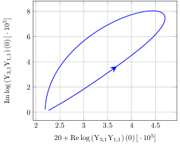
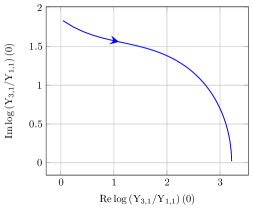
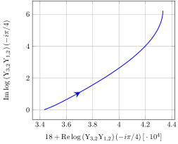
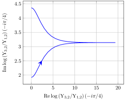
Figure 3: Paths of the driving terms during the analytic continuation for the path Eq.  (24). The starting values for the parameters chosen here are $|m_{1}|=10$, $|m_{2}|=9$, $C_{1}=\mathrm{arccosh}\left(\frac{3}{5}\right)$, $C_{2}=\mathrm{arccosh}\left(\frac{4}{7}\right)$. Note that some axes have been shifted and rescaled. The direction of growing $\varphi$ is indicated by the arrows.

4.2.1 Numerical analysis of the continuation

After finding the paths of continuation for the driving terms, we now turn to the determination of $\mathrm{A}_{\mathrm{free}}$. To do so, we need to determine those $\tilde{{\rm Y}}_{a,s}$-functions for which a solution to the equation $\tilde{{\rm Y}}_{a,s}=-1$ crosses the real axis, as explained in detail in section 3.3. Since we know the behavior of the system parameters in the new Y-system along the path of continuation, we can simply solve the Y-system in the complex $\theta$-plane for each value of $\varphi$ and then determine the location of the solutions $\tilde{{\rm Y}}_{a,s}=-1$. We solve the Y-system by an iterative procedure, similar to the algorithm presented in Alday:2010vh .

Following this procedure, we find the behavior for the $\tilde{{\rm Y}}$-functions displayed in figure 4.

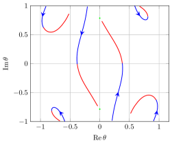
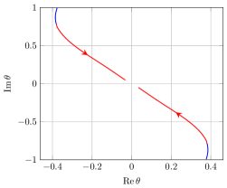
Figure 4: Left: Crossing solutions of $\tilde{{\rm Y}}_{3,2}(\theta)=-1$ during the continuation Eq.  (24). We find that two solutions cross the real axis and approach the endpoints $\pm i\frac{\pi}{4}$. Right: Towards the end of the continuation, a pair of solutions of $\tilde{{\rm Y}}_{2,2}(\theta)=-1$ approaches the real axis, but does not contribute to the remainder function as is argued in the main text. The direction of growing $\varphi$ is indicated by the arrows.

We see that a pair of solutions of $\tilde{{\rm Y}}_{3,2}$ crosses the real axis and approaches the values $\pm i\frac{\pi}{4}$ at the end of the continuation. Furthermore, two solutions of $\tilde{{\rm Y}}_{2,2}$ approach the origin at the end of the continuation. As we show in the next section, the Y-system equations for the triplet $\tilde{{\rm Y}}_{a,2}$ at the end of the continuation are of the same form as the equations for the $6$-point case in section 3.3. Therefore, we can argue as in the $6$-point case that the pair of solutions of $\tilde{{\rm Y}}_{2,2}$ never crosses the integration contour and we just have to consider the pair of crossing solutions of $\tilde{{\rm Y}}_{3,2}(\theta)$. Furthermore, since we find the same equations as in the $6$-point case for the triplet $\tilde{{\rm Y}}_{a,2}$, we can use the endpoint conditions Eq.(70) to analytically determine the endpoint of the Bethe roots to be $\pm i\frac{\pi}{4}$, confirming our numerical analysis.

4.2.2 Calculation of the remainder function

Using the input from the numerical analysis, we can now determine the amplitude. Let us stress again that the input from the numerics is discrete - it only provides information on which Y-functions have crossed. The endpoints can be determined analytically, therefore our result derived below is not bound to any numerical accuracy. Note also that since we are done with the numerical analysis, we can switch back to the standard Y-system Eqs. (37)-(39), because the crossing solutions of the $\tilde{{\rm Y}}$-functions are independent of the choice of system parameters, of course. As a first step, let us determine the cross ratios at the end of the continuation. In the following, all quantities that have been analytically continued are marked with a prime, as before. At the end of the continuation, the Y-system takes the following form:

$$\log\tilde{{\rm Y}}^{\prime}_{1,s} =-|m_{s}|^{\prime}\cosh\theta-C^{\prime}_{s}+\sum\limits_{a^{\prime},s^{\prime}}\int d\theta^{\prime}K_{s,s^{\prime}}^{1,a^{\prime}}\left(\theta-\theta^{\prime}+i\phi^{\prime}_{s}-i\phi^{\prime}_{s^{\prime}}\right)\log\left(1+\tilde{{\rm Y}}^{\prime}_{a^{\prime},s^{\prime}}(\theta^{\prime})\right)$$

$$+\log\frac{S_{s,2}^{1,3}(\theta+i\frac{\pi}{4}+i\phi^{\prime}_{s}-i\phi^{\prime}_{2})}{S_{s,2}^{1,3}(\theta-i\frac{\pi}{4}+i\phi^{\prime}_{s}-i\phi^{\prime}_{2})},$$ (92)

$$\log\tilde{{\rm Y}}^{\prime}_{2,s} =-\sqrt{2}|m_{s}|^{\prime}\cosh\theta+\sum\limits_{a^{\prime},s^{\prime}}\int d\theta^{\prime}K_{s,s^{\prime}}^{2,a^{\prime}}\left(\theta-\theta^{\prime}+i\phi^{\prime}_{s}-i\phi^{\prime}_{s^{\prime}}\right)\log\left(1+\tilde{{\rm Y}}^{\prime}_{a^{\prime},s^{\prime}}(\theta^{\prime})\right)$$

$$+\log\frac{S_{s,2}^{2,3}(\theta+i\frac{\pi}{4}+i\phi^{\prime}_{s}-i\phi^{\prime}_{2})}{S_{s,2}^{2,3}(\theta-i\frac{\pi}{4}+i\phi^{\prime}_{s}-i\phi^{\prime}_{2})},$$ (93)

$$\log\tilde{{\rm Y}}^{\prime}_{3,s} =-|m_{s}|^{\prime}\cosh\theta+C^{\prime}_{s}+\sum\limits_{a^{\prime},s^{\prime}}\int d\theta^{\prime}K_{s,s^{\prime}}^{3,a^{\prime}}\left(\theta-\theta^{\prime}+i\phi^{\prime}_{s}-i\phi^{\prime}_{s^{\prime}}\right)\log\left(1+\tilde{{\rm Y}}^{\prime}_{a^{\prime},s^{\prime}}(\theta^{\prime})\right)$$

$$+\log\frac{S_{s,2}^{3,3}(\theta+i\frac{\pi}{4}+i\phi^{\prime}_{s}-i\phi^{\prime}_{2})}{S_{s,2}^{3,3}(\theta-i\frac{\pi}{4}+i\phi^{\prime}_{s}-i\phi^{\prime}_{2})}.$$ (94)

As we now go to the multi-Regge limit, we can neglect the integrals and are left with the equations

$${\rm Y}^{\prime}_{1,s} =\left(e^{-|m_{s}|^{\prime}\cosh(\theta-i\phi^{\prime}_{s})-C^{\prime}_{s}}\right)\frac{S_{s,2}^{1,3}(\theta+i\frac{\pi}{4}-i\phi^{\prime}_{2})}{S_{s,2}^{1,3}(\theta-i\frac{\pi}{4}-i\phi^{\prime}_{2})},$$ (95)

$${\rm Y}^{\prime}_{2,s} =\left(e^{-\sqrt{2}|m_{s}|^{\prime}\cosh(\theta-i\phi^{\prime}_{s})}\right)\frac{S_{s,2}^{2,3}(\theta+i\frac{\pi}{4}-i\phi^{\prime}_{2})}{S_{s,2}^{2,3}(\theta-i\frac{\pi}{4}-i\phi^{\prime}_{2})},$$ (96)

$${\rm Y}^{\prime}_{3,s} =\left(e^{-|m_{s}|^{\prime}\cosh(\theta-i\phi^{\prime}_{s})+C^{\prime}_{s}}\right)\frac{S_{s,2}^{3,3}(\theta+i\frac{\pi}{4}-i\phi^{\prime}_{2})}{S_{s,2}^{3,3}(\theta-i\frac{\pi}{4}-i\phi^{\prime}_{2})}.$$ (97)

Using the recursion relations and introducing the parameters

$$\varepsilon^{\prime}:=e^{-|m_{s}|^{\prime}\cos\left((s-1)\frac{\pi}{4}+\phi^{\prime}_{s}\right)},\,w^{\prime}:=e^{|m_{s}|^{\prime}\sin\left((s-1)\frac{\pi}{4}+\phi^{\prime}_{s}\right)},$$ (98)

we find that the cross ratios at the end of the path are given by

$$u^{\prime}_{11} =1-\gamma\varepsilon^{\prime}_{2}\left(w^{\prime}_{2}+\frac{1}{w^{\prime}_{2}}-2\cosh C^{\prime}_{2}\right),\quad u^{\prime}_{21}=\gamma w^{\prime}_{2}\varepsilon^{\prime}_{2},\quad u^{\prime}_{31}=\gamma\frac{\varepsilon^{\prime}_{2}}{w^{\prime}_{2}},$$ (99)

$$u^{\prime}_{12} =1+\varepsilon^{\prime}_{1}\left(\frac{1}{\gamma}w^{\prime}_{1}+\frac{1}{w^{\prime}_{1}}+\frac{2}{\sqrt{-\gamma}}\sinh C^{\prime}_{1}\right),\quad u^{\prime}_{22}=-\frac{1}{\gamma}w^{\prime}_{1}\varepsilon^{\prime}_{1},\quad u^{\prime}_{32}=-\frac{\varepsilon^{\prime}_{1}}{w^{\prime}_{1}},$$

where $\gamma=-3-2\sqrt{2}$, and all above expressions are valid up to corrections of $\mathcal{O}(\varepsilon^{\prime 2})$. For the path under consideration we then impose $u^{\prime}_{22}=-u_{22}$, $u^{\prime}_{32}=-u_{32}$, as well as $u^{\prime}_{as}=u_{as}$ for all other cross ratios. This determines $\varepsilon^{\prime}_{s}$, $w^{\prime}_{s}$ and $C^{\prime}_{s}$ in terms of the old parameters, giving rise to the relations

$$\varepsilon^{\prime}_{1} =\sqrt{\gamma}\varepsilon_{1},\quad w^{\prime}_{1}=\sqrt{\gamma}w_{1},\quad \cosh C^{\prime}_{1}=\sqrt{1-\left(w_{1}+w_{1}^{-1}+\cosh C_{1}\right)^{2}},$$ (100)

$$\varepsilon^{\prime}_{2} =\frac{1}{\gamma}\varepsilon_{2},\quad w^{\prime}_{2}=w_{2},\quad \cosh C^{\prime}_{2}=-\cosh C_{2},$$

again up to corrections $\mathcal{O}(\varepsilon^{2})$. We can now examine the terms of the remainder function Eq. (52) after the continuation piece by piece and see how they contribute. We start with $\mathrm{A}_{\mathrm{per}}$, which after the continuation reads

$$\mathrm{A}^{\prime}_{\mathrm{per}}= \frac{1}{2}\left(\log^{2}\varepsilon^{\prime}_{1}+\log^{2}w^{\prime}_{1}+\log^{2}\varepsilon^{\prime}_{2}+\log^{2}w^{\prime}_{2}\right.$$ (101)

$$\quad\left.+\log\varepsilon^{\prime}_{1}\log\varepsilon^{\prime}_{2}+\log w^{\prime}_{1}\log w^{\prime}_{2}+\log\varepsilon^{\prime}_{2}\log w^{\prime}_{1}-\log\varepsilon^{\prime}_{1}\log w^{\prime}_{2}\right).$$

Using Eq.  (100), this gives

$$\mathrm{A}^{\prime}_{\mathrm{per}}=\mathrm{A}_{\mathrm{per}}+\frac{1}{4}\log^{2}\gamma-\frac{1}{2}\log\gamma\log\varepsilon_{2}.$$ (102)

We next turn to $\mathrm{A}_{\mathrm{free}}$. We determined the relevant crossings already in the last section. Furthermore, we know from section 3.3 that in the multi Regge-limit only the residue terms from the crossing $\tilde{{\rm Y}}$-functions contribute to the free energy. In the last section we saw that one pair of solutions of $\tilde{{\rm Y}}_{3,2}$ crosses the real axis and approaches the endpoints $\pm i\frac{\pi}{4}$. After neglecting the integrals, we are therefore left with

$$\mathrm{A}^{\prime}_{\mathrm{free}}= -\frac{|m_{2}|}{2\pi}\left(2\pi i\sinh\left(-i\frac{\pi}{4}\right)-2\pi i\sinh\left(i\frac{\pi}{4}\right)\right)$$

$$= -\sqrt{2}\sqrt{\log^{2}\varepsilon^{\prime}_{2}+\log^{2}w^{\prime}_{2}}$$ (103)

$$\approx +\sqrt{2}\log\varepsilon^{\prime}_{2}=+\sqrt{2}\left(\log\varepsilon_{2}-\log\gamma\right).$$

This leaves us with $\Delta^{\prime}$, whose form before continuation was spelled out in Eq.  (50). During the continuation, some cut contributions have to be picked up and we end up with

$$\Delta^{\prime}= \Delta-i\frac{\pi}{4}\left(2\log u_{11}+\log u_{12}+\log\tilde{u}-2\log(1-u_{11})\right)$$

$$+\frac{1}{4}\left(\mathrm{Li}_{2}(1-u_{22})-\mathrm{Li}_{2}(1+u_{22})+\mathrm{Li}_{2}(1-u_{32})-\mathrm{Li}_{2}(1+u_{32})\right)+\mathrm{const.}$$ (104)

$$= -i\frac{\pi}{2}\log\varepsilon_{2}-i\frac{\pi}{2}\log\left(w_{2}+w_{2}^{-1}+2\cosh C_{2}\right)+\mathrm{const.}+\mathcal{O}(\varepsilon).$$

Adding all contributions and using $\log\gamma=\log|\gamma|-i\pi$ we find

$$A^{\prime}_{\mathrm{per}}+A^{\prime}_{\mathrm{free}}+\Delta^{\prime}+i\delta^{\prime}_{7,--+}=-e_{2}\log\varepsilon_{2}-i\pi e_{2}+\mathrm{const.}+\mathcal{O}(\varepsilon),$$ (105)

where

$$e_{2}=-\sqrt{2}+\log\left(1+\sqrt{2}\right)$$ (106)

and where

$$\delta^{\prime}_{7,--+}=\frac{\pi}{2}\log\left(w_{2}+\frac{1}{w_{2}}+2\cosh C_{2}\right)$$ (107)

is a phase that cancels with an equivalent term in the BDS-part in the full amplitude. To rewrite this result in terms of the cross ratios we use the relations

$$\varepsilon_{2}=\sqrt{\tilde{u}_{21}\tilde{u}_{31}}(1-u_{11}),\quad w_{2}=\sqrt{\frac{u_{21}}{u_{31}}}$$ (108)

and obtain

$$A^{\prime}_{\mathrm{per}}+A^{\prime}_{\mathrm{free}}+\Delta^{\prime}+i\delta^{\prime}_{7,--+}=\frac{\sqrt{\lambda}}{2\pi}\left(e_{2}\log\left(-(1-u_{11})\tilde{u}_{21}\tilde{u}_{31}\right)+\mathrm{const.}\right).$$ (109)

Exponentiating, we obtain our final result for the remainder function

$$\left.e^{R_{7,--+}+i\delta_{7,--+}}\right|_{\mathrm{MRL}}\sim\left(-(1-u_{11})\sqrt{\tilde{u}_{21}\tilde{u}_{31}}\right)^{\frac{\sqrt{\lambda}}{2\pi}e_{2}},$$ (110)

where

$$\delta_{7,--+}=\frac{\sqrt{\lambda}}{2}\log\left(\tilde{u}_{21}\tilde{u}_{31}\right)=\frac{\pi}{2}\gamma_{K}\log\left(\tilde{u}_{21}\tilde{u}_{31}\right)$$ (111)

with the strong coupling limit of the cusp anomalous dimension $\gamma_{K}=\frac{\sqrt{\lambda}}{\pi}$. Remarkably, this result can be expressed in the same form as the $6$-point result, $R_{7,--+}(u_{as})=R_{6,--}(u_{11},u_{21},u_{31})$, and nicely matches the weak-coupling predictions as stated in section 2.4.

Note that in this section we have focused on the calculation for the region $P_{7,--+}$. The calculation for the region $P_{7,+--}$ is very similar and is therefore presented in appendix E. Here we only present the final result, which reads

$$e^{R_{7,+--}+i\delta_{7,+--}}\sim\left(-(1-u_{12})\sqrt{\tilde{u}_{22}\tilde{u}_{32}}\right)^{\frac{\sqrt{\lambda}}{2\pi}e_{2}},$$ (112)

with

$$\delta_{7,+--}=\frac{\pi}{2}\gamma_{K}\log\left(\tilde{u}_{22}\tilde{u}_{32}\right)$$ (113)

showing manifestly the target-projectile symmetry Eq.  (8) we have mentioned before.

4.3 Remainder function in the Regge region $(---)$

After having discussed the paths with only two flipped legs, we now turn to the path where all produced particles are chosen to be incoming. As explained in section 2, the naive continuation along (semi-)circles fails for this path as it does not satisfy the conformal Gram relation. An appropriate deformation that is consistent with the Gram relation was spelled out in Eq. (25) and this is the one we will be using throughout our analysis. As before, we use the recursion relations to determine the behavior of the driving terms of the modified Y-system Eqs.  (89)-(91). A plot of the curves followed by the driving terms during the continuation is shown in figure 5.

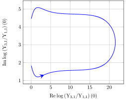
Figure 5: Solution of the driving terms during the continuation Eq.  (25). The direction of growing $\varphi$ is indicated by the arrows. For simplicity, the sets of parameters are identified as $|m|=|m_{1}|=|m_{2}|=10$, $C=C_{1}=-C_{2}=\mathrm{arccosh}\left(\frac{3}{5}\right)$ at the starting point.

4.3.1 Numerical analysis of the continuation

We then turn to the numerical analysis of $\mathrm{A}_{\mathrm{free}}$ for this Regge region. For the first time, we find that four solutions $\tilde{{\rm Y}}_{a,s}(\theta)=-1$ from two different Y-functions, namely $\tilde{{\rm Y}}_{3,1}$ and $\tilde{{\rm Y}}_{1,2}$, cross the real axis. The endpoints of these crossing solutions will be called $\theta_{12\pm}$ and $\theta_{31\pm}$, respectively. The corresponding crossing plots are shown in figure 6.

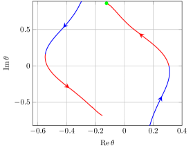
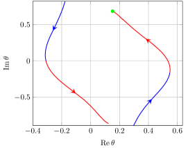
Figure 6: Crossing solutions of the functions $\tilde{{\rm Y}}_{1,2}(\theta)$ (left) and $\tilde{{\rm Y}}_{3,1}(\theta)$ (right) during the continuation Eq.  (25). The mirror symmetry $\tilde{{\rm Y}}_{1,2}(\theta)=\tilde{{\rm Y}}_{3,1}(-\theta)$ is due to our choice $|m_{1}|=|m_{2}|=10$, $C_{1}=-C_{2}=\mathrm{arccosh}\left(\frac{3}{5}\right)$ at the beginning of the continuation. The arrows indicate the direction of growing $\varphi$. We change colors once the first solution crosses the real axis.

From figure 6 it is obvious that difference of the two pairs of crossed Bethe roots is given by $i\frac{\pi}{2}$. However, their absolute position does not seem to be a special point in the $\theta$-plane. This is due to the relatively poor numerical convergence of the Y-functions for this particular path. In fact, while for all other paths studied so far mass parameters of the size of $\mathcal{O}(10)$ were enough to produce convergent Y-functions after only one iteration of the integral kernels, this is no longer true for this path. Therefore, the endpoints not ending on a distinguished point in the $\theta$-plane is a reflection of the fact that we are not close enough to the limit $|m_{s}|\rightarrow\infty$ yet. Indeed, if we study the endpoint position of the Bethe roots as a function of the initial mass parameter we find the results shown in figure 7 as we increase the initial mass parameters towards infinity. The result of the numerical analysis then is that we have four crossing Bethe roots, two ending at $+i\frac{\pi}{4}$ and two ending at $-i\frac{\pi}{4}$.

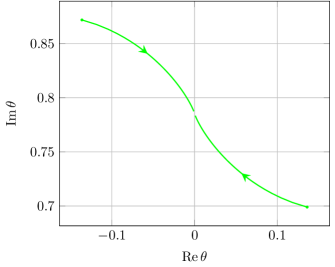
Figure 7: Convergence of the crossing solutions $\theta_{12+}$ and $\theta_{31+}$ against $i\frac{\pi}{4}$. The green dots indicate the position of the green dots in figure 6 and correspond to an initial value for the mass parameter of $|m_{1}|=|m_{2}|=10$. We then increase the initial mass parameter up to $|m_{1}|=|m_{2}|=2000$ until the convergence against $i\frac{\pi}{4}$ becomes obvious.

This numerical result can be backed up by analytical considerations as for the other paths. We begin by writing out the Y-system equations at the endpoint of the continuation:

$$\log\tilde{{\rm Y}}^{\prime}_{1,s}(\theta)= -|m_{s}|^{\prime}\cosh\theta-C^{\prime}_{s}+\sum\limits_{a^{\prime},s^{\prime}}\int d\theta^{\prime}K_{s,s^{\prime}}^{1,a^{\prime}}\left(\theta-\theta^{\prime}+i\phi^{\prime}_{s}-i\phi^{\prime}_{s^{\prime}}\right)\log\left(1+\tilde{{\rm Y}}^{\prime}_{a^{\prime},s^{\prime}}(\theta^{\prime})\right)$$

$$+\log\frac{S_{s,2}^{1,1}(\theta-\theta_{12-}+i\phi^{\prime}_{s}-i\phi^{\prime}_{2})}{S_{s,2}^{1,1}(\theta-\theta_{12+}+i\phi^{\prime}_{s}-i\phi^{\prime}_{2})}\frac{S_{s,1}^{1,3}(\theta-\theta_{31-}+i\phi^{\prime}_{s}-i\phi^{\prime}_{1})}{S_{s,1}^{1,3}(\theta-\theta_{31+}+i\phi^{\prime}_{s}-i\phi^{\prime}_{1})},$$ (114)

$$\log\tilde{{\rm Y}}^{\prime}_{2,s}(\theta)= -\sqrt{2}|m_{s}|^{\prime}\cosh\theta+\sum\limits_{a^{\prime},s^{\prime}}\int d\theta^{\prime}K_{s,s^{\prime}}^{2,a^{\prime}}\left(\theta-\theta^{\prime}+i\phi^{\prime}_{s}-i\phi^{\prime}_{s^{\prime}}\right)\log\left(1+\tilde{{\rm Y}}^{\prime}_{a^{\prime},s^{\prime}}(\theta^{\prime})\right)$$

$$+\log\frac{S_{s,2}^{2,1}(\theta-\theta_{12-}+i\phi^{\prime}_{s}-i\phi^{\prime}_{2})}{S_{s,2}^{2,1}(\theta-\theta_{12+}+i\phi^{\prime}_{s}-i\phi^{\prime}_{2})}\frac{S_{s,1}^{2,3}(\theta-\theta_{31-}+i\phi^{\prime}_{s}-i\phi^{\prime}_{1})}{S_{s,1}^{2,3}(\theta-\theta_{31+}+i\phi^{\prime}_{s}-i\phi^{\prime}_{1})},$$ (115)

$$\log\tilde{{\rm Y}}^{\prime}_{3,s}(\theta)= -|m_{s}|^{\prime}\cosh\theta+C^{\prime}_{s}+\sum\limits_{a^{\prime},s^{\prime}}\int d\theta^{\prime}K_{s,s^{\prime}}^{3,a^{\prime}}\left(\theta-\theta^{\prime}+i\phi^{\prime}_{s}-i\phi^{\prime}_{s^{\prime}}\right)\log\left(1+\tilde{{\rm Y}}^{\prime}_{a^{\prime},s^{\prime}}(\theta^{\prime})\right)$$

$$+\log\frac{S_{s,2}^{3,1}(\theta-\theta_{12-}+i\phi^{\prime}_{s}-i\phi^{\prime}_{2})}{S_{s,2}^{3,1}(\theta-\theta_{12+}+i\phi^{\prime}_{s}-i\phi^{\prime}_{2})}\frac{S_{s,1}^{3,3}(\theta-\theta_{31-}+i\phi^{\prime}_{s}-i\phi^{\prime}_{1})}{S_{s,1}^{3,3}(\theta-\theta_{31+}+i\phi^{\prime}_{s}-i\phi^{\prime}_{1})}.$$ (116)

From the standard two standard endpoint conditions $-1=\tilde{{\rm Y}}^{\prime}_{1,2}(\theta_{12\pm})=\tilde{{\rm Y}}^{\prime}_{3,1}(\theta_{31\pm})$, we only learn that

$$\theta_{12+}-\theta_{12-}=i\frac{\pi}{2}\quad\mathrm{and}\quad\theta_{31+}-\theta_{31-}=i\frac{\pi}{2}.$$ (117)

However, we can also take into account the finiteness of ratios of Y-functions at the endpoint of the continuation,

$$1 =\frac{\tilde{{\rm Y}}^{\prime}_{1,2}(\theta_{12-})}{\tilde{{\rm Y}}^{\prime}_{1,2}(\theta_{12+})}=-e^{|m_{2}|^{\prime}(\cosh\theta_{12+}+i\sinh\theta_{12+})}\left(\frac{1+\cosh(\theta_{12+}-\theta_{31+})+i\sinh(\theta_{12+}-\theta_{31+})}{1-\cosh(\theta_{12+}-\theta_{31+})-i\sinh(\theta_{12+}-\theta_{31+})}\right)$$

$$=\frac{\tilde{{\rm Y}}^{\prime}_{3,1}(\theta_{31-})}{\tilde{{\rm Y}}^{\prime}_{3,1}(\theta_{31+})}=-e^{|m_{1}|^{\prime}(\cosh\theta_{31+}+i\sinh\theta_{31+})}\left(\frac{1-\cosh(\theta_{12+}-\theta_{31+})-i\sinh(\theta_{12+}-\theta_{31+})}{1+\cosh(\theta_{12+}-\theta_{31+})+i\sinh(\theta_{12+}-\theta_{31+})}\right),$$ (118)

where we have already used Eq.  (117). As before, the S-matrix factors have to either diverge or go to zero as we send the mass parameters to infinity to give a finite product, depending on the sign of the exponent. However, we see that in Eq.  (118) the S-matrix factors of the two equations are inverses of each other. Therefore, one of the S-matrix factors has to go to zero, while the other diverges. This is satisfied if

$$\theta_{12+}=\theta_{31+}.$$ (119)

This leaves us with one undetermined endpoint. Taking the product of the two equations (118) and using Eq.  (119),

$$1=e^{(|m_{1}|^{\prime}+|m_{2}|^{\prime})\left(\cosh\theta_{12+}+i\sinh\theta_{12+}\right)},$$ (120)

we see that the driving term has to be zero which finally gives us $\theta_{12+}=\theta_{31+}=i\frac{\pi}{4}$. Although certainly more complicated than in the other cases studied so far, this is a very pleasing result, as it reinforces our belief that we only need discrete input from the numerical calculations and can calculate the endpoints analytically.

4.3.2 Calculation of the remainder function

We now have all the necessary information to calculate the remainder function $R_{7,---}$. As the calculation is similar to the one presented in section 4.2, we will be brief. First, we calculate the cross ratios from Eqs. (114)-(116) and obtain

$$u_{11}^{\prime}=1+\varepsilon_{2}^{\prime}\left(\frac{1}{w_{2}^{\prime}}+\gamma w_{2}^{\prime}+2\sqrt{-\gamma}\sinh C_{2}^{\prime}\right),\quad u_{21}^{\prime}=-\gamma w_{2}^{\prime}\varepsilon_{2}^{\prime},\quad u_{31}^{\prime}=-\frac{\varepsilon_{2}^{\prime}}{w_{2}^{\prime}},$$ (121)

$$u_{12}^{\prime}=1+\varepsilon_{1}^{\prime}\left(w_{1}^{\prime}+\frac{\gamma}{w_{1}^{\prime}}+2\sqrt{-\gamma}\sinh C_{1}^{\prime}\right),\quad u_{22}^{\prime}=-w_{1}^{\prime}\varepsilon_{1}^{\prime},\quad u_{31}^{\prime}=-\gamma\frac{\varepsilon_{1}^{\prime}}{w_{1}^{\prime}}.$$

After imposing the identification $u_{as}^{\prime}=u_{as}$, we find the new parameters to be given by

$$\varepsilon_{1}^{\prime}=\frac{\varepsilon_{1}}{\sqrt{\gamma}},\quad w_{1}^{\prime}=-\sqrt{\gamma}w_{1},\quad \cosh C_{1}^{\prime}=-\sinh C_{1},$$ (122)

$$\varepsilon_{2}^{\prime}=\frac{\varepsilon_{2}}{\sqrt{\gamma}},\quad w_{2}^{\prime}=-\frac{w_{2}}{\sqrt{\gamma}},\quad \cosh C_{2}^{\prime}=\sinh C_{2}.$$

Going through the different contributions of the amplitude, we find the following results:

$$A_{\mathrm{free}}^{\prime} \cong\sqrt{2}\log\varepsilon_{1}+\sqrt{2}\log\varepsilon_{2}-\sqrt{2}\log\gamma,$$ (123)

$$A_{\mathrm{per}}^{\prime}-A_{\mathrm{per}} \cong-\frac{1}{2}\left(i\pi+\log\gamma\right)\log\left(\varepsilon_{1}\varepsilon_{2}\right)-\frac{i\pi}{2}\log\left(\frac{w_{1}}{w_{2}}\right)+\mathrm{const.}$$ (124)

For $\Delta^{\prime}$, a small subtlety appears due to the non-trivial rotation of $\tilde{u}$, which gives rise to contributions $\sim\log(1-\tilde{u})$ and $\sim\log\tilde{u}$. $\tilde{u}$ appears explicitly in the answer. However, we will not replace it with an expression in terms of the $\varepsilon_{s}$ and $w_{s}$, but just use the fact that $1-\tilde{u}\sim\mathcal{O}(\varepsilon^{2})$ as can be seen from Eq.  (142). This allows us to drop the term $\sim\log\tilde{u}$ and we obtain

$$\Delta^{\prime}-\Delta\cong-i\frac{\pi}{2}\log\left(\varepsilon_{1}\varepsilon_{2}\right)+\frac{i\pi}{2}\log\left(\frac{w_{2}}{w_{1}}\right)-i\frac{\pi}{2}\log\left(1-\tilde{u}\right)+\mathrm{const.}$$ (125)

Putting all results together, and using $\log\gamma=\log\left|\gamma\right|-3i\pi$ we find for the remainder function

$$R_{7,---}+i\delta_{7,---}=\frac{\sqrt{\lambda}}{2\pi}\left(e_{2}\log\left(\varepsilon_{1}\varepsilon_{2}\right)+\mathrm{const.}\right),$$ (126)

which is just the sum of the remainder functions for the paths $P_{7,--+}$ and $P_{7,+--}$, presented in section 4.2 and appendix E, respectively. Exponentiating, we find our final result

$$\left.e^{R_{7,---}+i\delta_{7,---}}\right|_{\mathrm{MRL}}\sim\left((1-u_{11})(1-u_{12})\sqrt{\tilde{u}_{21}\tilde{u}_{31}\tilde{u}_{22}\tilde{u}_{32}}\right)^{\frac{\sqrt{\lambda}}{2\pi}e_{2}},$$ (127)

where

$$\delta_{7,---}=\frac{\sqrt{\lambda}}{4}\log\left(\frac{(1-u_{11})(1-u_{12})}{1-\tilde{u}}\sqrt{\tilde{u}_{21}\tilde{u}_{31}\tilde{u}_{22}\tilde{u}_{32}}\right)+\frac{\sqrt{\lambda}}{4}\log\left(\frac{\tilde{u}_{21}}{\tilde{u}_{31}}\frac{\tilde{u}_{32}}{\tilde{u}_{22}}\right).$$ (128)

This ends our study of this path and we turn to the last remaining Regge region.

4.4 Remainder function in the Regge region $(-+-)$

In section 2 we have identified four interesting Regge regions. The one we have not discussed so far is $P_{7,-+-}$, which we examine using the continuation

$$u_{11}(\varphi)=e^{2i\varphi}u_{11},\quad u_{21}(\varphi)=e^{-i\varphi}u_{21},\quad u_{31}(\varphi)=e^{i\varphi}u_{31},$$ (129)

$$u_{12}(\varphi)=e^{2i\varphi}u_{12},\quad u_{22}(\varphi)=e^{i\varphi}u_{22},\quad u_{32}(\varphi)=e^{-i\varphi}u_{32},\quad \tilde{u}(\varphi)=e^{-2i\varphi}\tilde{u}.$$

No deformation of paths is needed to satisfy the Gram relation and we can study the crossing solutions as before. However, for this particular path we see no crossing solutions. The Y-system equations therefore remain unmodified at the endpoint of the continuation, and the remainder function is trivial up to a phase,

$$\left.e^{R_{7,-+-}+i\delta_{7,-+-}}\right|_{\mathrm{MRL}}\sim 1,$$ (130)

with

$$\delta_{7,-+-}=\frac{\sqrt{\lambda}}{4}\log\left(\frac{1}{(1-\tilde{u})}\frac{1}{\tilde{u}_{22}\tilde{u}_{31}}\right),$$ (131)

which arises from the continuation of $\Delta$. This is a rather surprising result, as we expected to see a contribution of all three cuts, as predicted by the weak coupling analysis (cf. section 2.4). It may, however, be that our choice of path is too naive for this region. For example, it is conceivable that this region should rather be probed by first following the path $P_{7,---}$ and only then flipping the middle gluon back up. Since crossing solutions occur for $P_{7,---}$ it would be interesting to see if those solutions cross back to give the trivial result Eq.  (130) when flipping the middle gluon back up or if we find a different result. It should be noted that this issue is not present in the weak coupling description where the various regions can be studied without specifying a path which connects them.

5 Conclusions and outlook

In this paper, we have presented a general algorithm for the calculation of $n$-gluon scattering amplitudes in strongly coupled $\mathcal{N}=4$ SYM in various multi-Regge regions. It is based on the central observation that the multi-Regge limit of gauge theory corresponds to the infrared or large mass limit of the TBA equations that describe the strong coupling regime. In this limit, the quantum fluctuations of the one-dimensional auxiliary integrable system can be neglected which leads to drastic simplifications. In particular, the integral equations that describe excitations of the one-dimensional system are replaced by a set of algebraic Bethe Ansatz equations and the energy of excitations is evaluated as the sum of bare energies. These general observations are highly relevant for the evaluation of Regge cut contributions at strong coupling since such cut contributions can be argued to be associated with special excitations of the auxiliary one-dimensional quantum systems. Once the relevant solution of the Bethe Ansatz equations has been identified, one can build the associated Y-functions, reconstruct the cross ratios and compute the free energy and thereby the remainder function at strong coupling.

A crucial ingredient in this program is to decide which solution of the Bethe Ansatz is actually relevant for any given multi-Regge region. At the moment we do that by analytically continuing the cross ratios along a prescribed path and following the solutions of $\tilde{{\rm Y}}_{a,s}(\theta)=-1$ numerically. We characterized the paths in section 2.3. The main difficulty lies in finding paths which are compatible with the conformal Gram relations. Constructing these paths has to be done case-by-case so far and we showed an explicit example for the $7$-point case. Finding paths for a general number of gluons would require a better understanding of the conformal Gram relations for arbitrary $n$. The numerical analysis is explained in section 3. This analysis, too, has to be carried out for each Regge region separately. We would like to stress again that the numerical analysis just provides discrete data, namely which solutions $\tilde{{\rm Y}}_{a,s}(\theta)=-1$ cross the integration contour. The calculation of the remainder function is therefore not limited by numerical accuracy.

As specific examples of our algorithm, we calculate the $7$-gluon amplitude in four Regge regions. For the remainder functions $R_{7,--+}$, $R_{7,+--}$ and $R_{7,---}$ we find that the result can be expressed only using the functions which appear already in the $6$-gluon case for the region $R_{6,--}$. This is in remarkable agreement with the weak-coupling predictions presented in section 2.4 and strengthens the belief that the analytic structure of the scattering amplitude as predicted by Regge theory is preserved at any value of the coupling constant.

Our findings for the remainder function $R_{7,-+-}$ disagree with the weak-coupling predictions - while we obtain a trivial remainder function (up to a phase), we expected to find contributions of three Regge cuts. As stated in section 4.4, we think that this mismatch might arise because the path we have chosen is too naive. It may well be that instead of going to the region $(-+-)$ immediately, this particular region should rather be probed by a stepwise continuation, first going to the region $(---)$ and then flipping the middle gluon back up. Since we know that crossing solutions occur for the path $P_{7,---}$ it would be interesting to see whether those solutions cross back to give a trivial remainder function when flipping the middle gluon back up or whether the remainder function at strong coupling is indeed sensitive to the way the continuation is performed. This problem will be addressed in the future.

From our results, many ideas for future research emerge. For example, it would be very interesting to study the $8$-gluon amplitude. In this case it is expected from the weak-coupling perspective that in some Regge regions, the functions describing the $6$-gluon case are no longer sufficient to describe the remainder function. This is due to the appearance of a new state which physically corresponds to a bound state of three Reggeons. It would therefore be relevant to understand if and how this new state shows up from the strong coupling perspective. Furthermore, since our $7$-point results can be expressed through the functions appearing already in the $6$-point amplitude it would be interesting to see if our results can be related to the conjectured expressions of Basso:2014pla .

Appendix A Conformal Gram relations

For a general scattering process involving $n$ particles, there are $3n-10$ independent Mandelstam invariants. As we review in the main text, we can build many more Mandelstam invariants $p_{i}p_{j}$ from the $n$ four-momenta of the external gluons. Due to this mismatch, there have to be relations among these Lorentz invariants. To find additional relations, we have to recall that in a four-dimensional space there can be at most four linearly independent vectors. Every additional vector can then be expressed as a linear combination of these four basis vectors. Without loss of generality, let us choose the momentum vectors $p_{1},...,p_{4}$ to be a basis. We then have relations

$$\sum\limits_{i}^{1..4,l}c_{i}p_{i}\ =\ 0\ ,$$ (132)

for coefficients $c_{i}$ and $l=5,..,n-1$. Multiplication with $2p_{j}$ gives rise to relations among the Lorentz invariants. The condition that these relations have non-trivial solutions for the $c_{i}$ can be cast into a different form by writing down the $(n-1)\times(n-1)$-matrix of inner products of the momenta,

$$P\ =\ \begin{pmatrix}0&p_{1}p_{2}&p_{1}p_{3}&\cdots&p_{1}p_{n-1}\\ p_{2}p_{1}&0&p_{2}p_{3}&\cdots&p_{2}p_{n-1}\\ p_{3}p_{1}&p_{3}p_{2}&0&\cdots&p_{3}p_{n-1}\\ \vdots&\vdots&\vdots&\ddots&\vdots\\ p_{n-1}p_{1}&p_{n-1}p_{2}&p_{n-1}p_{3}&\cdots&0\end{pmatrix},$$ (133)

where the main diagonal contains only zeros, since we are scattering massless gluons. Since we chose $p_{1},...,p_{4}$ to be a basis, these vectors are linearly independent, which is equivalent to saying that the upper left $4\times 4$-minor

$$\begin{vmatrix}0&p_{1}p_{2}&p_{1}p_{3}&p_{1}p_{4}\\ p_{2}p_{1}&0&p_{2}p_{3}&p_{2}p_{4}\\ p_{3}p_{1}&p_{3}p_{2}&0&p_{3}p_{4}\\ p_{4}p_{1}&p_{4}p_{2}&p_{4}p_{3}&0\end{vmatrix}\neq 0$$ (134)

does not vanish. Linear dependence of additional vectors then translates into the statement that every $5\times 5$-minor we can build by adding a column and a row of Eq.  (133) to the minor Eq.  (134) has to vanish,

$$\begin{vmatrix}0&p_{1}p_{2}&p_{1}p_{3}&p_{1}p_{4}&p_{1}p_{k}\\ p_{2}p_{1}&0&p_{2}p_{3}&p_{2}p_{4}&p_{2}p_{k}\\ p_{3}p_{1}&p_{3}p_{2}&0&p_{3}p_{4}&p_{3}p_{k}\\ p_{4}p_{1}&p_{4}p_{2}&p_{4}p_{3}&0&p_{4}p_{k}\\ p_{l}p_{1}&p_{l}p_{2}&p_{l}p_{3}&p_{l}p_{4}&p_{l}p_{k}\\ \end{vmatrix}=0.$$ (135)

These relations are called Gram determinant relations. Since the coefficient matrix Eq.  (133) is symmetric, this gives rise to $\frac{1}{2}(n-4)(n-5)$ relations. In total, we then have

$$\frac{n(n-3)}{2}-\frac{(n-5)(n-4)}{2}\ =\ 3n-10$$ (136)

invariants left, which is exactly the number of independent variables.

This, however, is not good enough for our given problem. In the above description we have only considered Lorentz symmetry of the variables. However, since the remainder function in $\mathcal{N}=4$ SYM is dual conformal invariant, non-trivial kinematic information has to be expressed by conformal cross ratios. We therefore face the problem of writing down Gram relations that obey dual conformal symmetry. This problem is solved in Eden:2012tu .

As a first step, we change from momentum variables to the dual variables $p_{i}=x_{i-1}-x_{i}$. Of course, everything we said above still applies to these variables. We then lift four-dimensional momentum space to a six-dimensional space on which the four-dimensional dual conformal symmetry $\mathrm{SO}(4,2)$ is realized as rotation symmetry of the null vectors $X_{i}^{\mu}:=(1,x_{i}^{2},x_{i}^{\mu})$. Note that these vectors are denoted in light-cone coordinates, such that

$$X_{i}^{2}=2(1\cdot x_{i}^{2})-2x_{i}^{\mu}x_{i\mu}=0,$$ (137)

as well as

$$X_{i}\cdot X_{j}=x_{j}^{2}+x_{i}^{2}-2x_{i}\cdot x_{j}=\left(x_{i}-x_{j}\right)^{2}=x_{i,j}^{2}.$$ (138)

Since we are in six-dimensional space, at most six vectors $X_{i}$ can be linearly independent. Without loss of generality, we choose $X_{1},...,X_{6}$ as basis vectors. Following the same arguments as above, we find $\frac{1}{2}(n-5)(n-6)$ conditions of the form

$$\mathrm{Gram}(1,2,3,4,5,6,j,k)=0,$$ (139)

where the above notation indicates that the $7\times 7$-minor built from the six basis vectors as well as row $j$ and column $k$ vanishes. These relations give rise to polynomial equations in the $x^{2}_{i,j}$ which are dual conformally invariant by construction. Having found the relations in the $x^{2}_{i,j}$ we can use Eqs. (5)-(7) to rewrite the relations in terms of the cross ratios. For $n=7$ external gluons the only relation reads

$$a\tilde{u}^{2}+b\tilde{u}+c=0$$ (140)

with lengthy coefficients

$$a= u_{11}u_{12}\left(-1+u_{12}u_{21}+u_{11}u_{32}\right),$$ (141)

$$b= -\frac{1}{2}+u_{11}+\frac{1}{2}u_{11}u_{12}+u_{12}u_{21}-2u_{11}u_{12}u_{21}-u_{12}^{2}u_{21}+u_{22}-u_{11}u_{22}$$

$$-2u_{12}u_{21}u_{22}+u_{11}u_{12}u_{21}u_{22}+u_{12}^{2}u_{21}^{2}u_{22}-\frac{1}{2}u_{22}u_{31}+u_{12}u_{21}u_{22}u_{31}$$

$$+\frac{1}{2}u_{11}u_{12}u_{21}u_{32}+\frac{1}{2}u_{11}u_{12}u_{21}u_{22}u_{31}u_{32}+(\mathrm{target}\leftrightarrow\mathrm{projectile}),$$

$$c= \frac{1}{2}-u_{11}-u_{21}+u_{11}u_{21}+u_{12}u_{21}-u_{22}+u_{11}u_{22}+u_{21}u_{22}-u_{11}u_{21}u_{22}$$

$$+u_{12}u_{21}u_{22}-u_{12}u_{21}^{2}u_{22}+\frac{1}{2}u_{22}u_{31}+u_{21}u_{22}u_{31}-2u_{12}u_{21}u_{22}u_{31}$$

$$-u_{21}u_{22}^{2}u_{31}+u_{12}u_{21}^{2}u_{22}^{2}u_{31}+\frac{1}{2}u_{21}u_{32}-u_{11}u_{21}u_{32}-u_{21}u_{22}u_{31}u_{32}$$

$$+u_{11}u_{21}u_{22}u_{31}u_{32}+\frac{1}{2}u_{21}u_{22}^{2}u_{31}^{2}u_{32}+\left(\mathrm{target}\leftrightarrow\mathrm{projectile}\right),$$

where $\left(\mathrm{target}\leftrightarrow\mathrm{projectile}\right)$ means that the same expression after applying a target-projectile transformation (cf. Eq.  (8)), including the constant terms, should be added. This relation simplifies when approaching the multi-Regge limit. In fact, setting all small cross ratios to zero, $u_{2s}=u_{3s}=0$, in Eq.  (140) we find

$$0=(\tilde{u}-1)(1-u_{11}-u_{12}+u_{11}u_{12}\tilde{u}).$$ (142)

Appendix B The remainder function in the Euclidean regime

In this appendix we show that the remainder function of the $7$-point amplitude is trivial in the Euclidean region. To do so, we use Eqs. (61) and (55) to rewrite all contributions of the remainder function in terms of the variables $\varepsilon_{s}$ and $w_{s}$. Let us begin with $\mathrm{A}_{\mathrm{free}}$. Remember that in the large $|m_{s}|$-regime the integrals in Eqs. (37)-(39) can be neglected, which leads to the following schematic form of the integrals appearing in $\mathrm{A}_{\mathrm{free}}$:

$$\frac{|m_{s}|}{2\pi}\int d\theta\cosh\theta\log\left(1+\tilde{{\rm Y}}_{a,s}(\theta)\right)\approx\frac{|m_{s}|}{2\pi}\int d\theta\cosh\,\theta e^{-|m_{s}|\cosh\theta}=\frac{|m_{s}|}{\pi}K_{1}(|m_{s}|),$$ (143)

where $K_{1}(x)$ is a modified Bessel function of the second kind Abramowitz1972 . Using its large $x$-asymptotics,

$$xK_{1}(x)\sim\sqrt{\frac{\pi x}{2}}e^{-x},$$ (144)

as well as

$$|m_{s}|=\left(\log^{2}\varepsilon_{s}+\log^{2}w_{s}\right)^{\frac{1}{2}}\approx-\log\varepsilon_{s},$$ (145)

we see that the above integral Eq.  (143) is of $\mathcal{O}(\varepsilon\log\varepsilon)$ and therefore vanishes in the $\varepsilon\rightarrow 0$ limit. Hence, $\mathrm{A}_{\mathrm{free}}$ does not contribute in this limit. Next we study $\mathrm{A}_{\mathrm{per}}$. Starting from Eq.  (51) and using Eq.  (55), we find that

$$\mathrm{A}_{\mathrm{per}}= \frac{1}{2}\left(\log^{2}\varepsilon_{1}+\log^{2}w_{1}+\log^{2}\varepsilon_{2}+\log^{2}w_{2}\right.$$

$$\quad\left.+\log\varepsilon_{1}\log\varepsilon_{2}+\log w_{1}\log w_{2}+\log\varepsilon_{2}\log w_{1}-\log\varepsilon_{1}\log w_{2}\right).$$

For the last remaining term of the remainder function, $\mathrm{A}_{\mathrm{BDS-like}}-\mathrm{A}_{\mathrm{BDS}}$, we use Eq.  (61) in Eq.  (50), expand in $\varepsilon_{s}$ and keep only the leading terms, finding

$$\Delta= -\frac{\pi^{2}}{6}-\frac{1}{2}\left(\log^{2}\varepsilon_{1}+\log^{2}w_{1}+\log^{2}\varepsilon_{2}+\log^{2}w_{2}\right)$$ (146)

$$-\frac{1}{2}\left(\log\varepsilon_{1}\log\varepsilon_{2}-\log\varepsilon_{1}\log w_{2}+\log\varepsilon_{2}\log w_{1}+\log w_{1}\log w_{2}\right).$$

Summing all terms, we find that only a constant remainder function remains, as it must. It should be noted that this constant, $-\frac{\pi^{2}}{6}$, comes solely from the leading term in the expansion of the $\mathrm{Li}_{2}(1-u_{i})$, which occur with opposite sign in $\mathrm{A}_{\mathrm{BDS}}$. Hence, this constant will cancel in the full amplitude.

Appendix C Kernels of the rewritten Y-system

In this appendix we spell out the Y-system kernels $\mathcal{K}_{s,s^{\prime}}^{a,a^{\prime}}$ of the rewritten Y-system Eqs.  (89)-(91), which we use in the numerical analysis of $\mathrm{A}_{\mathrm{free}}$. $K_{i}(x)$ denote the kernels of the standard Y-system (cf. Eq.  (43)). In the following, $s\pm 1$ denotes the unique possible choice for $s^{\prime}$ in a given kernel. Furthermore, if a formula holds for both $a^{\prime}=1$ and $a^{\prime}=3$ we just write $a^{\prime}=2\pm 1$.

$$\mathcal{K}_{s,s}^{1,2\pm 1}(\theta,\theta^{\prime}) =K_{1}(\theta^{\prime})\cosh\theta-K_{1}(\theta-\theta^{\prime})$$

$$\mathcal{K}_{s,s}^{1,2}(\theta,\theta^{\prime}) =K_{2}(\theta^{\prime})\cosh\theta-K_{2}(\theta-\theta^{\prime})$$

$$\mathcal{K}_{s,s\pm 1}^{1,2}(\theta,\theta^{\prime}) =-K_{1}(-\theta^{\prime}+i\phi_{s}-i\phi_{s\pm 1})\cosh\theta+K_{1}(\theta-\theta^{\prime}+i\phi_{s}-i\phi_{s\pm 1})$$

$$\mathcal{K}_{s,s\pm 1}^{1,1}(\theta,\theta^{\prime}) =\frac{1}{2}\left(K_{2}(\theta-\theta^{\prime}+i\phi_{s}-i\phi_{s\pm 1})-K_{2}(-\theta^{\prime}+i\phi_{s}-i\phi_{s\pm 1})\cosh\theta\right)$$

$$\quad+\frac{1}{2}(-1)^{s+1}\left(K_{3}(\theta-\theta^{\prime}+i\phi_{s}-i\phi_{s\pm 1})-K_{3}(-\theta^{\prime}+i\phi_{s}-i\phi_{s\pm 1})\right)$$

$$\mathcal{K}_{s,s\pm 1}^{1,3}(\theta,\theta^{\prime}) =\frac{1}{2}\left(K_{2}(\theta-\theta^{\prime}+i\phi_{s}-i\phi_{s\pm 1})-K_{2}(-\theta^{\prime}+i\phi_{s}-i\phi_{s\pm 1})\cosh\theta\right)$$

$$\quad+\frac{1}{2}(-1)^{s}\left(K_{3}(\theta-\theta^{\prime}+i\phi_{s}-i\phi_{s\pm 1})-K_{3}(-\theta^{\prime}+i\phi_{s}-i\phi_{s\pm 1})\right)$$

$$\mathcal{K}_{s,s}^{2,2\pm 1}(\theta,\theta^{\prime}) =\sqrt{2}K_{1}(\theta^{\prime})\cosh\theta-K_{2}(\theta-\theta^{\prime})$$

$$\mathcal{K}_{s,s}^{2,2}(\theta,\theta^{\prime}) =\sqrt{2}K_{2}(\theta^{\prime})\cosh\theta-2K_{1}(\theta-\theta^{\prime})$$

$$\mathcal{K}_{s,s\pm 1}^{2,2}(\theta,\theta^{\prime}) =-\sqrt{2}K_{1}(-\theta^{\prime}+i\phi_{s}-i\phi_{s\pm 1})\cosh\theta+K_{2}(\theta-\theta^{\prime}+i\phi_{s}-i\phi_{s\pm 1})$$

$$\mathcal{K}_{s,s\pm 1}^{2,2\pm 1}(\theta,\theta^{\prime}) =-\frac{1}{\sqrt{2}}K_{2}(-\theta^{\prime}+i\phi_{s}-i\phi_{s\pm 1})\cosh\theta+K_{1}(\theta-\theta^{\prime}+i\phi_{s}-i\phi_{s\pm 1})$$

$$\mathcal{K}_{s,s}^{3,2\pm 1}(\theta,\theta^{\prime}) =K_{1}(\theta^{\prime})\cosh\theta-K_{1}(\theta-\theta^{\prime})$$

$$\mathcal{K}_{s,s}^{3,2}(\theta,\theta^{\prime}) =K_{2}(\theta^{\prime})\cosh\theta-K_{2}(\theta-\theta^{\prime})$$

$$\mathcal{K}_{s,s\pm 1}^{3,2}(\theta,\theta^{\prime}) =-K_{1}(-\theta^{\prime}+i\phi_{s}-i\phi_{s\pm 1})\cosh\theta+K_{1}(\theta-\theta^{\prime}+i\phi_{s}-i\phi_{s\pm 1})$$

$$\mathcal{K}_{s,s\pm 1}^{3,1}(\theta,\theta^{\prime}) =\frac{1}{2}\left(K_{2}(\theta-\theta^{\prime}+i\phi_{s}-i\phi_{s\pm 1})-K_{2}(-\theta^{\prime}+i\phi_{s}-i\phi_{s\pm 1})\cosh\theta\right)$$

$$\quad+\frac{1}{2}(-1)^{s}\left(K_{3}(\theta-\theta^{\prime}+i\phi_{s}-i\phi_{s\pm 1})-K_{3}(-\theta^{\prime}+i\phi_{s}-i\phi_{s\pm 1})\right)$$

$$\mathcal{K}_{s,s\pm 1}^{3,3}(\theta,\theta^{\prime}) =\frac{1}{2}\left(K_{2}(\theta-\theta^{\prime}+i\phi_{s}-i\phi_{s\pm 1})-K_{2}(-\theta^{\prime}+i\phi_{s}-i\phi_{s\pm 1})\cosh\theta\right)$$

$$\quad+\frac{1}{2}(-1)^{s+1}\left(K_{3}(\theta-\theta^{\prime}+i\phi_{s}-i\phi_{s\pm 1})-K_{3}(-\theta^{\prime}+i\phi_{s}-i\phi_{s\pm 1})\right)$$

Appendix D S-matrices

For the new set of kernels written out in appendix C, we have to determine the corresponding S-matrices. However, this is simple because the new kernels are linear combinations of the original kernels, possibly with prefactors. Therefore, the new S-matrices too should be given in terms of the original S-matrices Eqs. (65). Recall the original definition of the S-matrices,

$$-2\pi iK(\theta)=:\partial_{\theta}\log S(\theta).$$ (147)

Since the new kernels are now in general functions of both $\theta$, $\theta^{\prime}$ and not just their difference, we have to extend this definition in the following way:

$$-2\pi iK(\theta,\theta^{\prime})=:\partial_{\theta^{\prime}}\log S(\theta,\theta^{\prime})$$ (148)

This allows us to pick up the residue contributions in a very simple way, as before. Using this definition, we see that for a kernel of the schematic form

$$K(\theta,\theta^{\prime})=f(\theta)K_{1}(\theta,\theta^{\prime})+g(\theta)K_{2}(\theta,\theta^{\prime})+\dots$$ (149)

the S-matrix is given by

$$S(\theta,\theta^{\prime})=S_{1}(\theta,\theta^{\prime})^{f(\theta)}\cdot S_{2}(\theta,\theta^{\prime})^{g(\theta)}\cdot\dots$$ (150)

As a specific example, we spell out the S-matrices for a crossed solution of $\tilde{{\rm Y}}_{3,1}$ in the rewritten Y-system below:

$$S_{1,1}^{2,3}(\theta,\theta^{\prime}) =S_{1}(\theta^{\prime})^{\sqrt{2}\cosh\theta}S_{2}(\theta-\theta^{\prime})$$ (151)

$$S_{1,1}^{2\pm 1,3}(\theta,\theta^{\prime}) =S_{1}(\theta^{\prime})^{\cosh\theta}S_{1}(\theta-\theta^{\prime})$$

$$S_{2,1}^{1,3}(\theta,\theta^{\prime}) =\frac{S_{2}(-\theta^{\prime}+i\phi_{2}-i\phi_{1})^{\frac{1}{2}\cosh\theta}S_{3}(-\theta^{\prime}+i\phi_{2}-i\phi_{1})^{\frac{1}{2}}}{S_{2}(\theta-\theta^{\prime}+i\phi_{2}-i\phi_{1})^{\frac{1}{2}}S_{3}(\theta-\theta^{\prime}+i\phi_{2}-i\phi_{1})^{\frac{1}{2}}}$$

$$S_{2,1}^{2,3}(\theta,\theta^{\prime}) =S_{2}(\theta^{\prime}-i\phi_{2}+i\phi_{1})^{-\frac{1}{\sqrt{2}}\cosh\theta}S_{1}(\theta-\theta^{\prime}+i\phi_{2}-i\phi_{1})^{-1}$$

$$S_{2,1}^{3,3}(\theta,\theta^{\prime}) =\frac{S_{2}(-\theta^{\prime}+i\phi_{2}-i\phi_{1})^{\frac{1}{2}\cosh\theta}S_{3}(\theta-\theta^{\prime}+i\phi_{2}-i\phi_{1})^{\frac{1}{2}}}{S_{2}(\theta-\theta^{\prime}+i\phi_{2}-i\phi_{1})^{\frac{1}{2}}S_{3}(-\theta^{\prime}+i\phi_{2}-i\phi_{1})^{\frac{1}{2}}}$$

Similarly, we obtain all the other S-matrices from the kernels of appendix C. We refrain from spelling them out here explicitly.

Appendix E Remainder function in the Regge region $(+--)$

In this section we will briefly show the calculation for the path $P_{7,+--}$ of the cross ratios that was defined in Eq. (22). The calculation proceeds along the same steps as the one in section 4. Therefore, we only highlight the differences in the following. For the numerical analysis, we again have to determine the paths of the variables Eq.  (85) under the continuation Eq.  (22). We find the results depicted in figure 8.

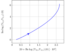
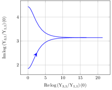
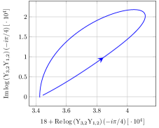
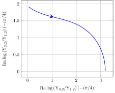
Figure 8: Continuation of the driving terms for the path Eq.  (22). Note that some axes have been rescaled and shifted. The direction of growing $\varphi$ is indicated by the arrows. The plots shown correspond to the parameter choice $|m_{1}|=10$, $|m_{2}|=9$, $C_{1}=\mathrm{arccosh}\left(\frac{3}{5}\right)$, $C_{2}=\mathrm{arccosh}\left(\frac{4}{7}\right)$ at the starting point.

Having found the paths of the driving terms, we can follow the solutions $\tilde{{\rm Y}}_{a,s}=-1$ during the continuation, leading to the results shown in figure 9.

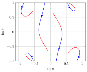
Figure 9: Paths followed by the solutions of $\tilde{{\rm Y}}_{3,1}(\theta)=-1$ during the continuation Eq.  (22). We find that one pair of solutions crosses the real axis. The direction of movement is indicated by arrows on the plot. We change the color of the curve when the pair of solutions crosses the integration contour.

We see that for the path $P_{7,+--}$, two solutions of $\tilde{{\rm Y}}_{3,1}$ cross the real axis and approach $\pm i\frac{\pi}{4}$, which can again be confirmed by an analytic argument using the endpoint conditions Eq.  (70). Furthermore, we find a pair of solutions of $\tilde{{\rm Y}}_{2,1}$ which approaches the real axis but never crosses. As before, these solutions do not contribute to the remainder function. Thus, after neglecting the integrals, the Y-system after the continuation is given by

$${\rm Y}^{\prime}_{1,s} =\left(e^{-|m_{s}|^{\prime}\cosh(\theta-i\phi^{\prime}_{s})-C^{\prime}_{s}}\right)\frac{S_{s,1}^{1,3}(\theta+i\frac{\pi}{4}-i\phi^{\prime}_{1})}{S_{s,1}^{1,3}(\theta-i\frac{\pi}{4}-i\phi^{\prime}_{1})},$$ (152)

$${\rm Y}^{\prime}_{2,s} =\left(e^{-\sqrt{2}|m_{s}|^{\prime}\cosh(\theta-i\phi^{\prime}_{s})}\right)\frac{S_{s,1}^{2,3}(\theta+i\frac{\pi}{4}-i\phi^{\prime}_{1})}{S_{s,1}^{2,3}(\theta-i\frac{\pi}{4}-i\phi^{\prime}_{1})},$$ (153)

$${\rm Y}^{\prime}_{3,s} =\left(e^{-|m_{s}|^{\prime}\cosh(\theta-i\phi^{\prime}_{s})+C^{\prime}_{s}}\right)\frac{S_{s,1}^{3,3}(\theta+i\frac{\pi}{4}-i\phi^{\prime}_{1})}{S_{s,1}^{3,3}(\theta-i\frac{\pi}{4}-i\phi^{\prime}_{1})},$$ (154)

with the S-matrices spelled out in appendix D. With this Y-system we determine the cross ratios after continuation to be

$$u^{\prime}_{11} =1+\varepsilon^{\prime}_{2}\left(w^{\prime}_{2}+\frac{1}{\gamma w^{\prime}_{2}}+2\frac{1}{\sqrt{-\gamma}}\sinh C^{\prime}_{2}\right),\quad u^{\prime}_{21}=-w^{\prime}_{2}\varepsilon^{\prime}_{2},\quad u^{\prime}_{31}=-\frac{1}{\gamma}\frac{\varepsilon^{\prime}_{2}}{w^{\prime}_{2}},$$

$$u^{\prime}_{12} =1-\gamma\varepsilon^{\prime}_{1}\left(w^{\prime}_{1}+\frac{1}{w^{\prime}_{1}}-2\cosh C^{\prime}_{1}\right),\quad u^{\prime}_{22}=\gamma w^{\prime}_{1}\varepsilon^{\prime}_{1},\quad u^{\prime}_{32}=\gamma\frac{\varepsilon^{\prime}_{1}}{w^{\prime}_{1}}.$$

Setting $u^{\prime}_{21}=-u_{21}$, $u^{\prime}_{31}=-u_{31}$ and $u^{\prime}_{as}=u_{as}$ for the remaining cross ratios we find

$$\varepsilon^{\prime}_{1} =\frac{1}{\gamma}\varepsilon_{1},\quad w^{\prime}_{1}=w_{1},\quad \cosh C^{\prime}_{1}=-\cosh C_{1},$$ (155)

$$\varepsilon^{\prime}_{2} =\sqrt{\gamma}\varepsilon_{2},\quad w^{\prime}_{2}=\frac{1}{\sqrt{\gamma}}w_{2},\quad \cosh C^{\prime}_{2}=\sqrt{1-\left(w_{2}+\frac{1}{w_{2}}+\cosh C_{2}\right)^{2}}$$

for the analytically continued auxiliary parameters. The rest of the calculation goes through as for the path $P_{7,--+}$ and we find the result

$$\left.e^{\mathrm{R_{7,+--}}+i\delta_{7,+--}}\right|_{\mathrm{MRL}}\sim\left(-(1-u_{12})\sqrt{\tilde{u}_{22}\tilde{u}_{32}}\right)^{\frac{\sqrt{\lambda}}{2\pi}e_{2}}$$ (156)

where

$$\delta_{7,+--}=\frac{\sqrt{\lambda}}{4}\log\left(\sqrt{\tilde{u}_{22}\tilde{u}_{32}}\right).$$ (157)

This result is consistent with the target-projectile symmetry which relates paths $P_{7,--+}$ and $P_{7,+--}$.

References

- (1) J. Bartels, V. Schomerus and M. Sprenger, JHEP 1410 (2014) 67 [arXiv:1405.3658 [hep-th]].
- (2) Z. Bern, L. J. Dixon and V. A. Smirnov, Phys. Rev. D 72 (2005) 085001 [hep-th/0505205].
- (3) L. F. Alday and J. Maldacena, JHEP 0711 (2007) 068 [arXiv:0710.1060 [hep-th]].
- (4) J. Bartels, L. N. Lipatov and A. Sabio Vera, Phys. Rev. D 80 (2009) 045002 [arXiv:0802.2065 [hep-th]].
- (5) J. Bartels, L. N. Lipatov and A. Sabio Vera, Eur. Phys. J. C 65 (2010) 587 [arXiv:0807.0894 [hep-th]].
- (6) A. B. Goncharov, M. Spradlin, C. Vergu and A. Volovich, Phys. Rev. Lett. 105 (2010) 151605 [arXiv:1006.5703 [hep-th]].
- (7) L. J. Dixon, J. M. Drummond, M. von Hippel and J. Pennington, JHEP 1312 (2013) 049 [arXiv:1308.2276 [hep-th]].
- (8) L. J. Dixon, J. M. Drummond, C. Duhr and J. Pennington, JHEP 1406 (2014) 116 [arXiv:1402.3300 [hep-th]].
- (9) S. Caron-Huot, JHEP 1112 (2011) 066 [arXiv:1105.5606 [hep-th]].
- (10) J. Golden and M. Spradlin, JHEP 1408 (2014) 154 [arXiv:1406.2055 [hep-th]].
- (11) B. Basso, A. Sever and P. Vieira, Phys. Rev. Lett. 111 (2013) 9, 091602 [arXiv:1303.1396 [hep-th]].
- (12) B. Basso, A. Sever and P. Vieira, JHEP 1401 (2014) 008 [arXiv:1306.2058 [hep-th]].
- (13) B. Basso, A. Sever and P. Vieira, JHEP 1408 (2014) 085 [arXiv:1402.3307 [hep-th]].
- (14) B. Basso, A. Sever and P. Vieira, JHEP 1409 (2014) 149 [arXiv:1407.1736 [hep-th]].
- (15) N. Beisert, C. Ahn, L. F. Alday, Z. Bajnok, J. M. Drummond, L. Freyhult, N. Gromov and R. A. Janik et al., Lett. Math. Phys. 99 (2012) 3 [arXiv:1012.3982 [hep-th]].
- (16) N. Gromov, V. Kazakov, S. Leurent and D. Volin, Phys. Rev. Lett. 112 (2014) 1, 011602 [arXiv:1305.1939 [hep-th]].
- (17) N. Gromov, V. Kazakov, S. Leurent and D. Volin, arXiv:1405.4857 [hep-th].
- (18) J. A. Minahan and K. Zarembo, JHEP 0303 (2003) 013 [hep-th/0212208].
- (19) N. Beisert, C. Kristjansen and M. Staudacher, Nucl. Phys. B 664 (2003) 131 [hep-th/0303060].
- (20) N. Beisert, Nucl. Phys. B 676 (2004) 3 [hep-th/0307015].
- (21) V. A. Kazakov, A. Marshakov, J. A. Minahan and K. Zarembo, JHEP 0405 (2004) 024 [hep-th/0402207].
- (22) J. M. Maldacena, Int. J. Theor. Phys. 38 (1999) 1113 [Adv. Theor. Math. Phys. 2 (1998) 231] [hep-th/9711200].
- (23) E. Witten, Adv. Theor. Math. Phys. 2 (1998) 253 [hep-th/9802150].
- (24) S. S. Gubser, I. R. Klebanov and A. M. Polyakov, Phys. Lett. B 428, 105 (1998) [hep-th/9802109].
- (25) G. Arutyunov, S. Frolov and M. Staudacher, JHEP 0410 (2004) 016 [hep-th/0406256].
- (26) N. Beisert and A. A. Tseytlin, Phys. Lett. B 629 (2005) 102 [hep-th/0509084].
- (27) R. Hernandez and E. Lopez, JHEP 0607 (2006) 004 [hep-th/0603204].
- (28) L. Freyhult and C. Kristjansen, Phys. Lett. B 638 (2006) 258 [hep-th/0604069].
- (29) N. Beisert, R. Hernandez and E. Lopez, JHEP 0611 (2006) 070 [hep-th/0609044].
- (30) N. Beisert, B. Eden and M. Staudacher, J. Stat. Mech. 0701 (2007) P01021 [hep-th/0610251].
- (31) L. F. Alday and J. M. Maldacena, JHEP 0706 (2007) 064 [arXiv:0705.0303 [hep-th]].
- (32) L. F. Alday and J. Maldacena, JHEP 0911 (2009) 082 [arXiv:0904.0663 [hep-th]].
- (33) L. F. Alday, D. Gaiotto and J. Maldacena, JHEP 1109 (2011) 032 [arXiv:0911.4708 [hep-th]].
- (34) L. F. Alday, J. Maldacena, A. Sever and P. Vieira, J. Phys. A 43 (2010) 485401 [arXiv:1002.2459 [hep-th]].
- (35) P. Heslop and V. V. Khoze, JHEP 1011 (2010) 035 [arXiv:1007.1805 [hep-th]].
- (36) T. Goddard, P. Heslop and V. V. Khoze, JHEP 1210 (2012) 041 [arXiv:1205.3448 [hep-th]].
- (37) M. A. C. Torres, Eur. Phys. J. C 74 (2014) 2757 [arXiv:1310.6906 [hep-th]].
- (38) J. C. Toledo, arXiv:1410.5896 [hep-th].
- (39) Y. Hatsuda, K. Ito, K. Sakai and Y. Satoh, JHEP 1009 (2010) 064 [arXiv:1005.4487 [hep-th]].
- (40) Y. Hatsuda, K. Ito, K. Sakai and Y. Satoh, JHEP 1104 (2011) 100 [arXiv:1102.2477 [hep-th]].
- (41) Y. Hatsuda, K. Ito and Y. Satoh, JHEP 1202 (2012) 003 [arXiv:1109.5564 [hep-th]].
- (42) Y. Hatsuda, K. Ito and Y. Satoh, JHEP 1302 (2013) 067 [arXiv:1211.6225 [hep-th]].
- (43) L. F. Alday, D. Gaiotto, J. Maldacena, A. Sever and P. Vieira, JHEP 1104 (2011) 088 [arXiv:1006.2788 [hep-th]].
- (44) D. Gaiotto, J. Maldacena, A. Sever and P. Vieira, JHEP 1103 (2011) 092 [arXiv:1010.5009 [hep-th]].
- (45) D. Gaiotto, J. Maldacena, A. Sever and P. Vieira, JHEP 1112 (2011) 011 [arXiv:1102.0062 [hep-th]].
- (46) A. Sever, P. Vieira and T. Wang, JHEP 1111 (2011) 051 [arXiv:1108.1575 [hep-th]].
- (47) A. Sever, P. Vieira and T. Wang, JHEP 1212 (2012) 065 [arXiv:1208.0841 [hep-th]].
- (48) B. Basso, A. Sever and P. Vieira, arXiv:1405.6350 [hep-th].
- (49) L. D. Faddeev and G. P. Korchemsky, Phys. Lett. B 342 (1995) 311 [hep-th/9404173].
- (50) L. N. Lipatov, hep-th/9311037.
- (51) V. S. Fadin and L. N. Lipatov, Phys. Lett. B 706 (2012) 470 [arXiv:1111.0782 [hep-th]].
- (52) L. N. Lipatov and A. Prygarin, Phys. Rev. D 83 (2011) 125001 [arXiv:1011.2673 [hep-th]].
- (53) L. J. Dixon, C. Duhr and J. Pennington, JHEP 1210 (2012) 074 [arXiv:1207.0186 [hep-th]].
- (54) B. Basso, S. Caron-Huot and A. Sever, arXiv:1407.3766 [hep-th].
- (55) J. Bartels, J. Kotanski and V. Schomerus, JHEP 1101 (2011) 096 [arXiv:1009.3938 [hep-th]].
- (56) J. Bartels, V. Schomerus and M. Sprenger, JHEP 1211 (2012) 145 [arXiv:1207.4204 [hep-th]].
- (57) J. Bartels, A. Kormilitzin and L. Lipatov, Phys. Rev. D 89 (2014) 065002 [arXiv:1311.2061 [hep-th]].
- (58) L. N. Lipatov, Theor. Math. Phys. 170 (2012) 166 [arXiv:1008.1015 [hep-th]].
- (59) J. Bartels, A. Kormilitzin and L. Lipatov, in preparation
- (60) J. Bartels, A. Kormilitzin and L. Lipatov, in preparation
- (61) J. Bartels, A. Kormilitzin, L. N. Lipatov and A. Prygarin, Phys. Rev. D 86 (2012) 065026 [arXiv:1112.6366 [hep-th]].
- (62) L. N. Lipatov, J. Phys. A 42 (2009) 304020 [arXiv:0902.1444 [hep-th]].
- (63) S. E. Derkachov and A. N. Manashov, J. Phys. A 47 (2014) 305204 [arXiv:1401.7477 [math-ph]].
- (64) G. Yang, JHEP 1012 (2010) 082 [arXiv:1004.3983 [hep-th]].
- (65) J. M. Drummond, J. Henn, G. P. Korchemsky and E. Sokatchev, Nucl. Phys. B 826 (2010) 337 [arXiv:0712.1223 [hep-th]].
- (66) G. Yang, JHEP 1103 (2011) 087 [arXiv:1006.3306 [hep-th]].
- (67) P. Dorey and R. Tateo, Nucl. Phys. B 482 (1996) 639 [hep-th/9607167].
- (68) P. Dorey and R. Tateo, Nucl. Phys. B 515 (1998) 575 [hep-th/9706140].
- (69) J. Bartels, J. Kotanski, V. Schomerus and M. Sprenger, arXiv:1311.1512 [hep-th].
- (70) B. Eden, P. Heslop, G. P. Korchemsky and E. Sokatchev, Nucl. Phys. B 862 (2012) 450 [arXiv:1201.5329 [hep-th]].
- (71) M. Abramowitz and I. A. Stegun, Eds. ‘Handbook of Mathematical Functions with Formulas, Graphs and Mathematical Tables’ Dover Publications (1972).