Hadronic vacuum polarization function
within dispersive approach to QCD

Abstract

The dispersive approach to quantum chromodynamics is applied to the study of the hadronic vacuum polarization function and associated quantities. This approach merges the intrinsically nonperturbative constraints, which originate in the kinematic restrictions on the respective physical processes, with corresponding perturbative input. The obtained hadronic vacuum polarization function agrees with pertinent lattice simulation data. The evaluated hadronic contributions to the muon anomalous magnetic moment and to the shift of the electromagnetic fine structure constant conform with recent assessments of these quantities.

I Introduction

The theoretical description of a number of the strong interaction processes is inherently based on the hadronic vacuum polarization function $\Pi(q^{2})$. In particular, this function plays a crucial role in the studies of inclusive $\tau$ lepton hadronic decay and of electron–positron annihilation into hadrons, that provides decisive self–consistency tests of quantum chromodynamics (QCD). At the same time, the function $\Pi(q^{2})$ enters in the analysis of the hadronic contributions to such quantities of precise particle physics as the muon anomalous magnetic moment and the running of the electromagnetic fine structure constant, that, in turn, puts strong limits on the effects due to a possible new fundamental physics beyond the standard model (SM). Additionally, the theoretical exploration of the aforementioned processes constitutes a natural framework for a thorough investigation of both perturbative and intrinsically nonperturbative aspects of hadron dynamics.

The strong interactions possess the feature of the asymptotic freedom, that makes it possible to apply perturbation theory to the study of ultraviolet behaviour of the function $\Pi(q^{2})$. However, there is still no rigorous method of theoretical description of hadron dynamics at low energies, which would have provided one with robust unabridged results. This fact eventually forces one to engage a variety of nonperturbative approaches in order to examine the strong interactions in the infrared domain. For example, an insight into the low–energy behaviour of the hadronic vacuum polarization function can be gained from such methods as, e.g., lattice simulations Lat1; Lat2; Lat3; Lat4, operator product expansion OPE1; OPE2; OPE3; OPE4; OPE5; OPE6, instanton liquid model NLCQM; ILM, and others.

Theoretical particle physics widely employs various methods based on the dispersion relations. In particular, the latter provide a source of the nonperturbative information about the low–energy hadron dynamics. Specifically, the dispersion relations, which render the kinematic restrictions on the relevant physical processes into the mathematical form, impose stringent constraints on the pertinent quantities [such as $\Pi(q^{2})$ and related functions], that should certainly be accounted for when one comes out of the applicability range of perturbation theory. These nonperturbative constraints have been merged with corresponding perturbative input in the framework of dispersive approach to QCD DQCD1a; PRD88, which provides unified integral representations for the functions on hand, see Sec. II.

The primary objective of this paper is to calculate the hadronic vacuum polarization function within dispersive approach and to compare it with relevant lattice simulation data, as well as to evaluate the corresponding hadronic contributions to the muon anomalous magnetic moment and to the shift of the electromagnetic fine structure constant.

The layout of the paper is as follows. In Sec. II the dispersive approach to QCD DQCD1a; PRD88 is overviewed. Section LABEL:Sect:Latt presents the comparison of the hadronic vacuum polarization function calculated in the framework of dispersive approach with pertinent lattice simulation data and elucidates the qualitative distinctions between the approach on hand, its massless limit, and perturbative approach. Section LABEL:Sect:EW contains the evaluation of hadronic contributions to the aforementioned electroweak observables. In the Conclusions (Sect. LABEL:Sect:Concl) the basic results are summarized and further studies within this approach are outlined. Auxiliary material is given in the Appendix.

II Dispersive approach to Quantum Chromodynamics

The hadronic vacuum polarization function $\Pi(q^{2})$ is defined as the scalar part of the hadronic vacuum polarization tensor

$$\Pi_{\mu\nu}(q^{2})=i\!\int\!d^{4}x\,e^{iqx}\langle 0|\,T\!\left\{J_{\mu}(x)\,J_{\nu}(0)\right\}|0\rangle=\frac{i}{12\pi^{2}}(q_{\mu}q_{\nu}-g_{\mu\nu}q^{2})\Pi(q^{2}).$$ (1)

The kinematics of the process on hand determines the cut structure of $\Pi(q^{2})$ in the complex $q^{2}$–plane. Specifically, the function $\Pi(q^{2})$ (1) has the only cut along the positive semiaxis of real $q^{2}$ starting at the hadronic production threshold $4m_{\pi}^{2}=m^{2}$ (discussion of this issue can be found in, e.g., Ref. Feynman, as well as in Refs. DQCD1a; PRD88; DQCDPrelim1). Proceeding from this fact and bearing in mind the asymptotic ultraviolet behaviour of the hadronic vacuum polarization function one can write down the corresponding dispersion relation by making use of the once–subtracted Cauchy integral formula [see Eq. (2) below]. For practical purposes it proves to be convenient to define the Adler function $D(Q^{2})$ Adler [see Eq. (6) below] and the related function $R(s)$, which is identified with the so–called $R$–ratio of electron–positron annihilation into hadrons [see Eq. (4) below]. Eventually, the complete set of well–known relations, which express the functions $\Pi(q^{2})$, $R(s)$, and $D(Q^{2})$ in terms of each other, acquires the following form (see papers Adler; PDisp; RKP82 as well as PRD88 and references therein):

$$\Delta\Pi(q^{2}\!,\,q_{0}^{2}) = (q^{2}-q_{0}^{2})\int_{m^{2}}^{\infty}\frac{R(\sigma)}{(\sigma-q^{2})(\sigma-q_{0}^{2})}\,d\sigma\qquad$$ (2)

$$= -\int_{-q_{0}^{2}}^{-q^{2}}D(\zeta)\frac{d\zeta}{\zeta},$$ (3)

$$R(s) = \frac{1}{2\pi i}\lim_{\varepsilon\to 0_{+}}\!\Delta\Pi(s+i\varepsilon,s-i\varepsilon)$$ (4)

$$= \frac{1}{2\pi i}\lim_{\varepsilon\to 0_{+}}\int_{s+i\varepsilon}^{s-i\varepsilon}D(-\zeta)\,\frac{d\zeta}{\zeta},$$ (5)

$$D(Q^{2}) = -\frac{d\,\Pi(-Q^{2})}{d\ln Q^{2}}$$ (6)

$$= Q^{2}\int_{m^{2}}^{\infty}\frac{R(\sigma)}{(\sigma+Q^{2})^{2}}\,d\sigma.\qquad$$ (7)

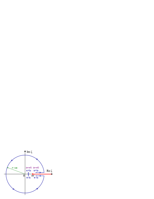
Figure 1: The integration contour in Eq. (5). The physical cut $\zeta\geq m^{2}$ of the Adler function $D(-\zeta)$ (6) is shown along the positive semiaxis of real $\zeta$.

In Eqs. (2)–(7) $\Delta\Pi(q^{2}\!,\,q_{0}^{2})=\Pi(q^{2})-\Pi(q_{0}^{2})$, whereas $Q^{2}=-q^{2}>0$ and $s=q^{2}>0$ denote the spacelike and timelike kinematic variables, respectively. The common prefactor $N_{\text{\scriptsize c}}\sum_{f=1}^{n_{\text{\tiny f}}}Q_{f}^{2}$ is omitted throughout the paper, where $N_{\text{\scriptsize c}}=3$ is the number of colours, $Q_{f}$ stands for the electric charge of $f$–th quark (in units of the elementary charge $e$), and $n_{\text{\scriptsize f}}$ denotes the number of active flavours. The integration contour in Eq. (5) lies in the region of analyticity of its integrand (see Fig. 1). Note that the derivation of relations (2)–(7) requires the knowledge of the cut structure of hadronic vacuum polarization function $\Pi(q^{2})$ (1) and its asymptotic ultraviolet behaviour. It is worth mentioning also that Eqs. (2) and (7) can be used for extracting the functions $\Delta\Pi(q^{2}\!,\,q_{0}^{2})$ and $D(Q^{2})$ from the experimental data on $R(s)$.

As noted in the Introduction, the dispersion relations (2)–(7) embody the kinematic restrictions on the respective physical processes and impose intrinsically nonperturbative constraints on the functions $\Pi(q^{2})$, $R(s)$, and $D(Q^{2})$, that should certainly be taken into account when one oversteps the limits of applicability of perturbation theory. These nonperturbative constraints have been merged with corresponding perturbative input in the framework of dispersive approach to QCD DQCD1a; PRD88, which provides the following unified integral representations for the functions on hand:

$$\Delta\Pi(q^{2},\,q_{0}^{2}) = \Delta\Pi^{(0)}(q^{2},\,q_{0}^{2})+\!\int_{m^{2}}^{\infty}\rho(\sigma)\ln\biggl{(}\frac{\sigma-q^{2}}{\sigma-q_{0}^{2}}\frac{m^{2}-q_{0}^{2}}{m^{2}-q^{2}}\biggr{)}\frac{d\,\sigma}{\sigma},$$ (8)

$$R(s) = R^{(0)}(s)+\theta(s-m^{2})\int_{s}^{\infty}\!\rho(\sigma)\frac{d\,\sigma}{\sigma},$$ (9)

$$D(Q^{2}) = D^{(0)}(Q^{2})+\frac{Q^{2}}{Q^{2}+m^{2}}\int_{m^{2}}^{\infty}\rho(\sigma)\frac{\sigma-m^{2}}{\sigma+Q^{2}}\frac{d\,\sigma}{\sigma}.$$ (10)

These equations have been obtained by employing the relations (2)–(7) and the asymptotic ultraviolet behaviour of the hadronic vacuum polarization function. In Eqs. (8)–(10) $\rho(\sigma)$ is the spectral density

$$\rho(\sigma) = \frac{1}{2\pi i}\frac{d}{d\,\ln\sigma}\lim_{\varepsilon\to 0_{+}}\Bigl{[}p(\sigma-i\varepsilon)-p(\sigma+i\varepsilon)\Bigr{]}$$

$$= -\frac{d}{d\,\ln\sigma}\,r(\sigma)$$

$$= \frac{1}{2\pi i}\lim_{\varepsilon\to 0_{+}}\Bigl{[}d(-\sigma-i\varepsilon)-d(-\sigma+i\varepsilon)\Bigr{]}\!,$$

$p(q^{2})$, $r(s)$, and $d(Q^{2})$ denote the strong corrections to the functions $\Pi(q^{2})$, $R(s)$, and $D(Q^{2})$, respectively, $\theta(x)$ stands for the unit step–function [$\theta(x)=1$ if $x\geq 0$ and $\theta(x)=0$ otherwise], and the leading–order terms read Feynman; QEDAB:

$$\Delta\Pi^{(0)}(q^{2},\,q_{0}^{2}) = 2\,\frac{\varphi-\tan\varphi}{\tan^{3}\varphi}-2\,\frac{\varphi_{0}-\tan\varphi_{0}}{\tan^{3}\varphi_{0}},$$ (12)

$$R^{(0)}(s) = \theta(s-m^{2})\biggl{(}1-\frac{m^{2}}{s}\biggr{)}^{\!\!3/2},$$ (13)

$$D^{(0)}(Q^{2}) = 1+\frac{3}{\xi}\Bigl{[}1-\sqrt{1+\xi^{-1}}\,\sinh^{-1}\!\bigl{(}\xi^{1/2}\bigr{)}\Bigr{]}\!,$$ (14)

where $\sin^{2}\!\varphi=q^{2}/m^{2}$, $\sin^{2}\!\varphi_{0}=q^{2}_{0}/m^{2}$, and $\xi=Q^{2}/m^{2}$, see papers DQCD1a; PRD88 and references therein for the details.

It is worthwhile to outline that the Adler function obtained in the framework of the dispersive approach (10) agrees with its experimental prediction in the entire energy range, see Refs. DQCD1a; DQCD1b; DQCD2. At the same time, the representations (8)–(10) conform with the results of Bethe–Salpeter calculations PRL99PRD77 as well as of lattice simulations RCTaylor. Additionally, the dispersive approach has proved to be capable of describing OPAL (update 2012, Ref. OPAL9912) and ALEPH (update 2014, Ref. ALEPH0514) experimental data on inclusive $\tau$ lepton hadronic decay in vector and axial–vector channels in a self–consistent way PRD88; QCD14 (see also Refs. DQCD3; C12).

In the framework of the approach on hand the corresponding perturbative input is accounted for in the same way as in other similar approaches, namely, by means of the spectral density (II). Specifically, the latter is approximated by its perturbative part, which can be calculated by making use of the perturbative expression for either of the strong corrections $p(q^{2})$, $r(s)$, and $d(Q^{2})$, see, e.g., papers CPC; BCmath and references therein:

(15)