Optimal nonlinear information processing capacity in delay-based reservoir computers

Abstract

Reservoir computing is a recently introduced brain-inspired machine learning paradigm capable of excellent performances in the processing of empirical data. We focus in a particular kind of time-delay based reservoir computers that have been physically implemented using optical and electronic systems and have shown unprecedented data processing rates. Reservoir computing is well-known for the ease of the associated training scheme but also for the problematic sensitivity of its performance to architecture parameters. This article addresses the reservoir design problem, which remains the biggest challenge in the applicability of this information processing scheme. More specifically, we use the information available regarding the optimal reservoir working regimes to construct a functional link between the reservoir parameters and its performance. This function is used to explore various properties of the device and to choose the optimal reservoir architecture, thus replacing the tedious and time consuming parameter scannings used so far in the literature.

Key Words: Reservoir computing, echo state networks, neural computing, time-delay reservoir, memory capacity, architecture optimization.

The increase in need for information processing capacity, as well as the physical limitations of the Turing or von Neumann machine methods implemented in most computational systems, has motivated the search for new brain-inspired solutions some of which present an outstanding potential. An important direction in this undertaking is based on the use of the intrinsic information processing abilities of dynamical systems [Crut 10] which opens the door to high performance physical realizations whose behavior is ruled by these structures [Caul 10, Wood 12].

The contributions in this paper take place in a specific implementation of this idea that is obtained as a melange of a recently introduced machine learning paradigm known under the name of reservoir computing (RC) [Jaeg 01, Jaeg 04, Maas 02, Maas 11, Croo 07, Vers 07, Luko 09] with a realization based on the sampling of the solution of a time-delay differential equation [Roda 11, Guti 12]. We refer to this combination as time-delay reservoirs (TDRs). Physical implementations of this scheme carried out with dedicated hardware are already available and have shown excellent performances in the processing of empirical data: spoken digit recognition [Jaeg 07, Appe 11, Larg 12, Paqu 12, Brun 13], the NARMA model identification task [Atiy 00, Roda 11], continuation of chaotic time series, and volatility forecasting [Grig 14]. A recent example that shows the potential of this combination are the results in [Brun 13] where an optoelectronic implementation of a TDR is capable of achieving the lowest documented error in the speech recognition task at unprecedented speed in an experiment design in which digit and speaker recognition are carried out in parallel.

A major advantage of RC is the linearity of its training scheme. This choice makes its implementation easy when compared to more traditional machine learning approaches like recursive neural networks, which usually require the solution of convoluted and sometimes ill-defined optimization problems. In exchange, as it can be seen in most of the references quoted above, the system performance is not robust with respect to the choice of the parameter values $\boldsymbol{\theta}$ of the nonlinear kernel used to construct the RC (see below). More specifically, small deviations from the optimal parameter values can seriously degrade the performance and moreover, the optimal parameters are highly dependent on the task at hand. This observation makes the kernel parameter optimization a very important step in the RC design and has motivated the introduction of alternative parallel-based architectures [Orti 12, Grig 14] to tackle this difficulty.

The main contribution of this paper is the introduction of an approximated model that, to our knowledge, provides the first rigorous analytical description of the delay-based RC performance. This powerful theoretical tool can be used to systematically study the delay-based RC properties and to replace the trial and error approach in the choice of architecture parameters by well structured optimization problems. This method simplifies enormously the implementation effort and sheds new light on the mechanisms that govern this information processing technique.

TDRs are based on the interaction of the time-dependent input signal $z(t)\in\mathbb{R}$ that we are interested in with the solution space of a time-delay differential equation of the form

$$\dot{x}(t)=-x(t)+f(x(t-\tau),I(t),\boldsymbol{\theta}),$$ (1)

where $f$ is a nonlinear smooth function (we call it nonlinear kernel) that depends on the $K$ parameters in the vector $\boldsymbol{\theta}\in\mathbb{R}^{K}$, $\tau>0$ is the delay, $x(t)\in\mathbb{R}$, and $I(t)\in\mathbb{R}$ is obtained using a temporal multiplexing over the delay period of the input signal $z(t)$ that we explain later on. We note that, even though the differential equation takes values in the real line, its solution space is infinite dimensional since an entire function $x\in C^{1}([-\tau,0],\mathbb{R})$ needs to be specified in order to initialize it. The choice of nonlinear kernel is determined by the intended physical implementation of the computing system; we focus on two parametric sets of kernels that have already been explored in the literature, namely, the Mackey-Glass [Mack 77] and the Ikeda [Iked 79] families. These kernels were used for reservoir computing purposes in the RC electronic and optic realizations in [Appe 11] and [Larg 12], respectively.

In order to visualize the TDR construction using a neural networks approach it is convenient, as in [Appe 11, Guti 12], to consider the Euler time-discretization of (1) with integration step $d:=\tau/N$, namely,

$$\frac{x(t)-x(t-d)}{d}=-x(t)+f(x(t-\tau),I(t),\boldsymbol{\theta}).$$ (2)

The design starts with the choice of a number $N\in\mathbb{N}$ of virtual neurons and of an adapted input mask ${\bf c}\in\mathbb{R}^{N}$. Next, the input signal $z(t)$ at a given time $t$ is multiplexed over the delay period by setting $\mathbf{I}(t):={\bf c}z(t)\in\mathbb{R}^{N}$ (see module A in Figure 1). We then organize it, as well as the solutions of (2), in neuron layers $\mathbf{x}(t)$ parametrized by a discretized time $t\in\mathbb{Z}$ by setting

$$x_{i}(t):=x(t\tau-(N-i)d),\quad I_{i}(t):=I(t\tau-(N-i)d),\quad i\in\{1,\ldots,N\},\quad t\in\mathbb{Z},$$

where $x_{i}(t)$ and $I_{i}(t)$ stand for the $i$th-components of the vectors $\mathbf{x}(t)$ and $\mathbf{I}(t)$, respectively, with $t\in\mathbb{Z}$. We say that $x_{i}(t)$ is the $i$th neuron value of the $t$th layer of the reservoir and $d$ is referred to as the separation between neurons. With this convention, the solutions of (2) are described by the following recursive relation:

$$x_{i}(t):=e^{-\xi}x_{i-1}(t)+(1-e^{-\xi})f(x_{i}(t-1),I_{i}(t),\boldsymbol{\theta}),\enspace\mbox{with}\enspace x_{0}(t):=x_{N}(t-1),\enspace\mbox{and}\enspace\xi:=\log(1+d),$$ (3)

that shows how, as depicted in module B in Figure 1, any neuron value is a convex linear combination of the previous neuron value in the same layer and a nonlinear function of both the same neuron value in the previous layer and the input. The weights of this combination are determined by the separation between neurons; when the distance $d$ is small, the neuron value $x_{i}(t)$ is mainly influenced by the previous neuron value $x_{i-1}(t)$, while large distances between neurons give predominance to the previous layer and foster the input gain. The recursions (3) uniquely determine a smooth map $F:\mathbb{R}^{N}\times\mathbb{R}^{N}\times\mathbb{R}^{K}\rightarrow\mathbb{R}^{N}$ that specifies the neuron values as a recursion on the neuron layers via an expression of the form

$$\mathbf{x}(t)=F(\mathbf{x}(t-1),\mathbf{I}(t),\boldsymbol{\theta}),$$ (4)

where $F$ is constructed out of the nonlinear kernel map $f$ that depends on the $K$ parameters in the vector $\boldsymbol{\theta}$; $F$ is referred to as the reservoir map.

The construction of the TDR computer is finalized by connecting, as in Module C of Figure 1, the reservoir output to a linear readout ${\bf W}_{{\rm out}}\in\mathbb{R}^{N}$ that is calibrated using a training sample by minimizing the associated task mean square error via a linear regression. We will refer to the module B in Figure 1 as the reservoir or the time-delay reservoir (TDR) and to the collection of the three modules as the reservoir computer (RC) or the TDR computer. A TDR based on the direct sampling of the solutions of (1) will be called a continuous time TDR and those based on the recursion (4) will be referred to as discrete time TDRs.

Figure 1: Neural diagram representing the architecture of the time-delay reservoir (TDR) and the three modules of the reservoir computer (RC): A is the input layer, B is the time-delay reservoir, and C is the readout layer.

As we already mentioned, the performance of the RC for a given task is much dependent on the value of the kernel parameters $\boldsymbol{\theta}$ and, in some cases, on the entries of the input mask ${\bf c}$ used for signal multiplexing. The optimal parameters $\boldsymbol{\theta}$ are usually determined by trial and error or using computationally costly systematic scannings that are by far the biggest burden at the time of adapting the RC to a new task. In this paper we construct an approximate model that we use to allows us to establish a functional link between the RC performance and the parameters $\boldsymbol{\theta}$ and the input mask values ${\bf c}$. Given a specific task, this explicit expression can be used to find appropriate parameter and mask values by solving a well structured and algorithmically convenient optimization problem that readily provides them.

The construction of this approximated formula is based on the observation that the optimal RC performance is always obtained when the TDR is working in a stable unimodal regime, that is, the reservoir is initialized at a stable equilibrium of the autonomous system ($I(t)=0$) associated to (1) and the mean and variance of the input signal $I(t)$ are designed using the input mask ${\bf c}$ so that the reservoir output remains around it and does not visit other stable equilibria or dynamical elements. In the next section we provide empirical and theoretical arguments for this claim. The performance measures that we consider in our study are the nonlinear memory capacities introduced in [Damb 12] as a generalization of the linear concept proposed in [Jaeg 02, Whit 04, Gang 08, Herm 10].

1 Results

1.1 Optimal performance: stability and unimodality

Stability and the reservoir defining properties.

The estimations of the RC performance using the nonlinear memory capacity that we present later on, consist of approximating the reservoir by its partial linearization at the level of the delayed self feedback term and of respecting the nonlinearity in the input injection. This approach is only acceptable when the optimal dynamical regime that we are interested in, remains close to a given point. A natural candidate for such qualitative behavior could be obtained by initializing the reservoir at an asymptotically stable equilibrium of the autonomous system associated to (1) and by controlling the mean and the variance of the input signal $I(t)$ so that the reservoir output remains close to it.

There is both theoretical and empirical evidence that suggests that optimal performance is obtained when working in a statistically stationary regime around a stable equilibrium. Indeed, one of the defining features of RC, namely the echo state property is materialized for general RCs by enforcing that the spectral radius of the internal connectivity matrix of the reservoir is smaller than one [Maas 02, Jaeg 04, Luko 09], which is the critical stability value for a quiescent state of the network when operating autonomously (without external injected information). It is well-known that the translation of this condition for TDRs implies parameter settings that ensure the existence of a stable state of (1) when $I(t)$ is set to zero. This feature typically relates to gains of the feedback smaller than the Hopf threshold of the delay dynamics or, equivalently, to a sufficiently low feedback rate so that self-sustained oscillations are avoided.

Asymptotic stability is closely related with the so-called fading memory property [Boyd 85, Maas 02]: the impact of any past injected input necessarily vanishes after a transient whose duration is typically of the order of the absolute value of the inverse of the smallest negative real part in the Lyapunov exponents. When the feedback gain is set too close to zero, the RC does not exhibit a long enough transient and thus presents an intrinsic memory that is too short to secure the self mixing of the temporal information necessary for its processing. On the other hand, if the feedback gain is set too close to the instability threshold, the input information flow requires too much time to vanish and hence the fading memory property is poorly satisfied. We recall the well known fact (see Section 8.2 in [Boyd 85]) that the fading memory property can be realized by input-output systems generated by time-delay differential equations only when these exhibit a unique stable equilibrium.

In the context of recent successful physical realizations of RC, experimental parameters are systematically chosen so that the conditions described above are satisfied. Indeed, in [Appe 11, Larg 12] these conditions are ensured via a proper tuning of the gain of the delayed feedback function. This approach differs from the one in [Brun 13], where the conditions are met by choosing a laser injection current strictly smaller but close to the lasing threshold, as well as by using a moderate feedback, which prevents eventual self sustained external cavity mode oscillations. An additional important observation suggested by all these experimental setups is the need for a nonlinearity at the level of the input injection. In [Appe 11, Larg 12] this feature is obtained using a strong enough input signal amplitude and via the transformation associated to the nonlinear delayed feedback. In [Brun 13] the delayed feedback is linear but an external Mach-Zehnder modulator is used that implicitly provides a nonlinear transformation of the input signal as it is optically seeded through the nonlinear electro-optic modulation transfer function of the Mach-Zehnder.

Stability analysis of the time-delay reservoir.

Due to the central role played by stability in our discussion, we now carefully analyze various sufficient conditions that ensure that the RC is functioning in a stable regime. All the statements that follow are carefully proved in the Supplementary Material section. Consider first an equilibrium $x_{0}\in\mathbb{R}$ of the continuous time model (1) working in autonomous regime, that is, we set $I(t)=0$. It can be shown using a Lyapunov-Krasovskiy-type analysis [Kras 63, Wu 10] that the asymptotic stability of $x_{0}$ is guaranteed whenever there exists an $\varepsilon>0$ and a constant $|k_{\varepsilon}|<1$ such that either

(i)

$f(x+x_{0},0,\boldsymbol{\theta})\leq k_{\varepsilon}x+x_{0}$ for all $x\in\left(-\varepsilon,\varepsilon\right)$, or

(ii)

$\dfrac{f(x+x_{0},0,\boldsymbol{\theta})-x_{0}}{x}\leq k_{\varepsilon}$ for all $x\in\left(-\varepsilon,\varepsilon\right)$.

The first condition can be used to prove the stability of equilibria exhibited by TDRs created using concave (but not necessarily differentiable) nonlinear kernels. As to the second one, it shows that if $f$ is differentiable at $x_{0}$ then this point is stable as long as $|\partial_{x}f(x_{0},0,\boldsymbol{\theta})|<1$, with $\partial_{x}f(x_{0},0,\boldsymbol{\theta})$ the first derivative of the nonlinear kernel $f$ in (1) with respect to the first argument at the point $(x_{0},0,\boldsymbol{\theta})$.

The stability study can also be carried out by working with the discrete-time approximation (4) of the TDR which is determined by the reservoir map $F:\mathbb{R}^{N}\times\mathbb{R}^{N}\times\mathbb{R}^{K}\rightarrow\mathbb{R}^{N}$. More specifically, it can be shown that $x_{0}\in\mathbb{R}$ is an equilibrium of (1) if and only if $\mathbf{x}_{0}:=(x_{0},\ldots,x_{0})^{\top}\in\mathbb{R}^{N}$ is a fixed point of (4). The asymptotic stability of this fixed point is ensured whenever the linearization $D_{\mathbf{x}}F(\mathbf{x}_{0},{\bf 0}_{N},\boldsymbol{\theta})$, which is a $N\times N$ matrix that will be referred to as the connectivity matrix, has a spectral radius smaller than one. Since it is not possible to compute the eigenvalues of $D_{\mathbf{x}}F(\mathbf{x}_{0},{\bf 0}_{N},\boldsymbol{\theta})$ for an arbitrary number of neurons $N$, we are hence obliged to proceed by finding estimations for the Cauchy bound [Rahm 02] of its characteristic polynomial or by bounding the spectral radius $\rho(D_{\mathbf{x}}F(\mathbf{x}_{0},{\bf 0}_{N},\boldsymbol{\theta}))$ using either a matrix norm or the Gershgorin discs [Horn 13]. An in-depth study of all these options showed that it is the use of the maximum row sum matrix norm $|||\cdot|||_{\infty}$ that yields the best stability bounds via the following statement:

$$\rho(D_{\mathbf{x}}F(\mathbf{x}_{0},{\bf 0}_{N},\boldsymbol{\theta}))\leq|||D_{\mathbf{x}}F(\mathbf{x}_{0},{\bf 0}_{N},\boldsymbol{\theta})|||_{\infty}<1\quad\mbox{if and only if}\quad|\partial_{{x}}f(x_{0},0,\boldsymbol{\theta})|<1.$$ (5)

Notice that this remarkable result puts together the stability conditions for the continuous and discrete time systems.

As an example of application of these results, consider the Mackey-Glass nonlinear kernel [Mack 77]

$$f(x,I,\boldsymbol{\theta})=\frac{\eta\left(x+\gamma I\right)}{1+\left(x+\gamma I\right)^{p}},$$ (6)

where the parameter $\boldsymbol{\theta}:=(\gamma,\eta,p)$ is a three tuple of real values; $\gamma$ is usually referred to as the input gain and $\eta$ the feedback gain. When this prescription is used in (1) in the autonomous regime, that is, $I(t)=0$, the associated dynamical system exhibits two families of equilibria $x_{0}$ parametrized by $\eta$, namely, $x_{0}=0$ and the roots of $x_{0}^{p}=\eta-1$. For example, in the case $p=2$, two distinct cases arise: when $\eta<1$ there is a unique equilibrium at the origin which is stable as long as $\eta\in(-1,1)$. When $\eta>1$ two other equilibria appear at $x_{0}=\pm\left(\eta-1\right)^{1/2}$ which are stable whenever $\eta<3$. These statements are proved in Corollary D.6 of the Supplementary Material. Analogous statements for the Ikeda kernel [Iked 79] $f(x,I,\boldsymbol{\theta})=\eta\sin^{2}\left(x+\gamma I+\phi\right)$, $\boldsymbol{\theta}:=(\eta,\gamma,\phi)$ can be found in Corollary D.7 of the Supplementary Material. A particularly convenient sufficient condition is $|\eta|\leq 1$ that simultaneously ensures stability and unimodality (existence of a single stable equilibrium).

Empirical evidence.

In order to confirm these theoretical and experimental arguments, we have carried out several numerical simulations in which we studied the RC performance in terms of the dynamical regime of the reservoir at the time of carrying out various nonlinear memory tasks. More specifically, we construct a reservoir using the Ikeda nonlinear kernel with $N=20$, $d=0.2581$, $\eta=1.2443$, $\gamma=1.4762$, and $\phi=0.1161$. The equilibria of the associated autonomous system are given by the points $x_{0}$ where the curves $y=x$ and $y=\eta\sin^{2}\left(x+\phi\right)$ intersect. With this parameter values, intersections take place at $x_{0}=0.0244$, $x_{0}=0.9075$, and $x_{0}=1.063$, which makes multi modality possible. As it can be shown with the results in the Supplementary Material section (see Corollary D.7), the first and the third equilibria are stable. In order to verify that the optimal performance is obtained when the RC operates in the neighborhood of a stable equilibrium, we study the normalized mean square error (NMSE) exhibited by a TDR initialized at $x_{0}=0.0244$ when we present to it a quadratic memory task. More specifically, we inject in a TDR an independent and identically normally distributed signal $z(t)$ with mean zero and variance $10^{-4}$ and we then train a linear readout ${\bf W}_{{\rm out}}$ (obtained with a ridge penalization of $\lambda=10^{-15}$) in order to recover the quadratic function $z(t-1)^{2}+z(t-2)^{2}+z(t-3)^{2}$ out of the reservoir output. The top left panel in Figure 2 shows how the NMSE behaves as a function of the mean and the variance of the input mask ${\bf c}$. It is clear that by modifying any of these two parameters we control how far the reservoir dynamics separates from the stable equilibrium, which we quantitatively evaluate in the two bottom panels by representing the RC performance in terms of the mean and the variance of the resulting reservoir output. Both panels depict how the injection of a signal slightly shifted in mean or with a sufficiently high variance results in reservoir outputs that separate from the stable equilibrium and in a severely degraded performance. An important factor in this deterioration seems to be the multi modality, that is, if the shifting in mean or the input signal variance are large enough then the reservoir output visits the stability basin of the other stable point placed at $x_{0}=1.063$; in the top right and bottom panels we have marked with red color the values for which bimodality has occurred so that the negative effect of this phenomenon is noticeable. In the Supplementary Material section we illustrate how the behavior that we just described is robust with respect to the choice of nonlinear kernel and is similar when the experiment is carried out using the Mackey-Glass function.

Figure 2: Behavior of the reservoir performance in a quadratic memory task as a function of the mean and the variance of the input mask. The modification of any of these two parameters influences how the reservoir dynamics separates from the stable equilibrium. The top panels show how the performance degrades very quickly as soon as the mean and the variance of the input mask (and hence of the input signal) separate from zero. The bottom panels depict the reservoir performance as a function of the various output means and variances obtained when changing the input means and variances. In the top right and bottom panels we have indicated with red markers the cases in which the reservoir visits the stability basin of a contiguous stable equilibrium hence showing how unimodality is associated to optimal performance.

1.2 The approximating model and the nonlinear memory capacity of the reservoir computer

The findings just presented have major consequences in the theoretical tools available for the evaluation of the RC performance. Indeed, since we now know that optimal operation is attained when the TDR functions in a unimodal fashion around an asymptotically stable steady state, we can approximate it by its partial linearization with respect to the delayed self feedback term at that point and keeping the nonlinearity for the input injection. For statistically independent input signals of the type used to compute nonlinear memory capacities of the type introduced in [Damb 12], this approximation allows us to visualize the TDR as a $N$-dimensional ($N$ is the number of neurons) vector autoregressive stochastic process of order one [Lutk 05] (we denote it as VAR(1)) for which the value of the associated nonlinear memory capacities can be explicitly computed. As we elaborate later on in the discussion, the quality of this approximation at the time of evaluating the memory capacities of the original system is excellent and the resulting function can be hence used for RC optimization purposes regarding the nonlinear kernel parameter values $\boldsymbol{\theta}$ and the input mask ${\bf c}$.

Consider a stable equilibrium $x_{0}\in\mathbb{R}$ of the autonomous system associated to (1) or, equivalently, a stable fixed point of (4) of the form $\mathbf{x}_{0}:=(x_{0},\ldots,x_{0})^{\top}\in\mathbb{R}^{N}$. If we approximate (4) by its partial linearization at $\mathbf{x}_{0}$ with respect to the delayed self feedback and by the $R$-order Taylor series expansion of the functional that describes the signal injection, we obtain an expression of the form:

$$\mathbf{x}(t)=F(\mathbf{x}_{0},{\bf 0}_{N},\boldsymbol{\theta})+A(\mathbf{x}_{0},\boldsymbol{\theta})(\mathbf{x}(t-1)-\mathbf{x}_{0})+\boldsymbol{\varepsilon}(t),$$ (7)

where $A(\mathbf{x}_{0},\boldsymbol{\theta}):=D_{\mathbf{x}}F(\mathbf{x}_{0},{\bf 0}_{N},\boldsymbol{\theta})$ is the linear connectivity matrix and $\boldsymbol{\varepsilon}(t)$ is given by:

$$\boldsymbol{\varepsilon}(t)=(1-{e}^{-\xi})\left(q_{R}\left(z(t),c_{1}\right),q_{R}\left(z(t),c_{1},c_{2}\right),\ldots,q_{R}\left(z(t),c_{1},\dots,c_{N}\right)\right)^{\top},$$ (8)

with

$$q_{R}\left(z(t),c_{1},\dots,c_{r}\right):=\sum^{R}_{i=1}\dfrac{z(t)^{i}}{i!}(\partial_{{I}}^{(i)}f)({x}_{0},0,\boldsymbol{\theta}){\sum^{r}_{j=1}{e}^{-(r-j)\xi}c_{j}^{i}},$$ (9)

and $(\partial_{{I}}^{(i)}f)({x}_{0},0,\boldsymbol{\theta})$ is the $i$th order partial derivative of the nonlinear kernel $f$ with respect to the second argument $I(t)$, evaluated at the point $({x}_{0},0,\boldsymbol{\theta})$.

If we now use as input signal ${z}(t)$ independent and identically distributed random variables with mean $0$ and variance $\sigma_{z}^{2}$ (we denote it by $\left\{{z}(t)\right\}_{t\in\mathbb{Z}}\sim{\rm IID}(0,\sigma_{z}^{2})$) then the recursion (7) makes the reservoir layer dynamics $\{\mathbf{x}(t)\}_{t\in\mathbb{Z}}$ into a discrete time random process that, as we show in what follows, is the solution of a $N$-dimensional vector autoregressive model of order 1 (VAR(1)). Indeed, it is easy to see that the assumption $\left\{{z}(t)\right\}_{t\in\mathbb{Z}}\sim{\rm IID}(0,\sigma_{z}^{2})$ implies that $\left\{\mathbf{I}(t)\right\}_{t\in\mathbb{Z}}\sim{\rm IID}({\bf 0}_{N},\Sigma_{I})$, with $\Sigma_{I}:=\sigma_{z}^{2}{\bf c}^{\top}{\bf c}$, and that $\{\boldsymbol{\varepsilon}(t)\}_{t\in\mathbb{Z}}$ is a family of $N$-dimensional independent and identically distributed random variables with mean $\boldsymbol{\mu}_{{\varepsilon}}$ and covariance matrix $\Sigma_{{\varepsilon}}$ given by the following expressions:

$$\boldsymbol{\mu}_{{\varepsilon}}={\rm E}\left[\boldsymbol{\varepsilon}(t)\right]=(1-{e}^{-\xi})\left(q_{R}\left(\mu_{{z}},c_{1}\right),q_{R}\left(\mu_{{z}},c_{1},c_{2}\right),\ldots,q_{R}\left(\mu_{{z}},c_{1},\dots,c_{N}\right)\right)^{\top},$$ (10)

where the polynomial $q_{R}$ is the same as in (9) and where we use the convention that the powers $\mu_{{z}}^{i}:={\rm E}\left[z(t)^{i}\right]$, for any $i\in\left\{1,\dots,R\right\}$ and with ${\rm E}[\cdot]$ denoting the mathematical expectation. Additionally, $\Sigma_{{\varepsilon}}:={\rm E}\left[(\boldsymbol{\varepsilon}(t)-\boldsymbol{\mu}_{{\varepsilon}})(\boldsymbol{\varepsilon}(t)-\boldsymbol{\mu}_{{\varepsilon}})^{\top}\right]$ has entries determined by the relation:

$$(\Sigma_{{\varepsilon}})_{ij}=(1-{e}^{-\xi})^{2}((q_{R}(\cdot,c_{1},\dots,c_{i})\cdot q_{R}(\cdot,c_{1},\dots,c_{j}))(\mu_{{z}})-q_{R}(\mu_{{z}},c_{1},\dots,c_{i})q_{R}(\mu_{{z}},c_{1},\dots,c_{j})),$$

where the first summand stands for the multiplication of the polynomials $q_{R}(\cdot,c_{1},\dots,c_{i})$ and $q_{R}(\cdot,c_{1},\dots,c_{j})$ and the subsequent evaluation of the resulting polynomial at $\mu_{z}$, and the second one is made out of the multiplication of the evaluation of the two polynomials.

Using these observations, we can consider (7) as the prescription of a VAR(1) model driven by the independent noise $\{\boldsymbol{\varepsilon}(t)\}_{t\in\mathbb{Z}}$. If the nonlinear kernel $f$ satisfies the generic condition that the polynomial in $u$ given by $\det\left(\mathbb{I}_{N}-A(\mathbf{x}_{0},\boldsymbol{\theta})u\right)$, does not have roots in and on the complex unit circle, then (7) has a second order stationary solution [Lutk 05, Proposition 2.1] $\{\mathbf{x}(t)\}_{t\in\mathbb{Z}}$ with time-independent mean given by

$$\boldsymbol{\mu}_{{x}}={\rm E}\left[\mathbf{x}(t)\right]=(I_{N}-A(\mathbf{x}_{0},\boldsymbol{\theta}))^{-1}(F(\mathbf{x}_{0},{\bf 0}_{N},\boldsymbol{\theta})-A(\mathbf{x}_{0},\boldsymbol{\theta})\mathbf{x}_{0}+\boldsymbol{\mu}_{{\varepsilon}})$$ (11)

and an also time independent autocovariance function $\Gamma(k):={\rm E}\left[\left(\mathbf{x}(t)-\boldsymbol{\mu}_{{x}}\right)\left(\mathbf{x}(t-k)-\boldsymbol{\mu}_{{x}}\right)^{\top}\right]$, $k\in\mathbb{Z}$, recursively determined the Yule-Walker equations (see [Lutk 05] for a detailed presentation). Indeed, $\Gamma(0)$ is given by the vectorized equality:

$${\rm vec}(\Gamma(0))=\left(\mathbb{I}_{N^{2}}-A(\mathbf{x}_{0},\boldsymbol{\theta})\otimes A(\mathbf{x}_{0},\boldsymbol{\theta})\right)^{-1}{\rm vec}(\Sigma_{{\varepsilon}}),$$ (12)

which determines the higher order autocovariances via the relation $\Gamma(k)=A(\mathbf{x}_{0},\boldsymbol{\theta})\Gamma(k-1)$ and the identity $\Gamma(-k)=\Gamma(k)^{\top}$. As we explain in the following paragraphs, the moments (10), (11), and (12) are all that is needed in order to characterize the memory capacities of the RC.

A $h$-lag memory task is determined by a (in general nonlinear) function $H:\mathbb{R}^{h+1}\rightarrow\mathbb{R}$ that is used to generate a one-dimensional signal $y(t):=H(z(t),z(t-1),\ldots,z(t-h))$ out of the reservoir input. Given a TDR computer, the optimal linear readout ${\mathbf{W}}_{{\rm out}}$ adapted to the memory task $H$ is given by the solution of a ridge linear regression problem with regularization parameter $\lambda\in\mathbb{R}$ (usually tuned during the training phase via cross-validation) in which the covariates are the neuron values corresponding to the reservoir output and the explained variables are the values $\{y(t)\}$ of the memory task function. The $H$-memory capacity $C_{H}(\boldsymbol{\theta},{\bf c},\lambda)$ of the TDR computer under consideration characterized by a nonlinear kernel $f$ with parameters $\boldsymbol{\theta}$, an input mask ${\bf c}$, and a regularizing ridge parameter $\lambda$ is defined as one minus the normalized mean square error committed at the time of accomplishing the memory task $H$. When the reservoir is approximated by a VAR(1) process, then the corresponding $H$-memory capacity is given by

$$C_{H}(\boldsymbol{\theta},{\bf c},\lambda)=\frac{{\rm Cov}(y(t),\mathbf{x}(t))^{\top}(\Gamma(0)+\lambda\mathbb{I}_{N})^{-1}(\Gamma(0)+2\lambda\mathbb{I}_{N})(\Gamma(0)+\lambda\mathbb{I}_{N})^{-1}{\rm Cov}(y(t),\mathbf{x}(t))}{{\rm var}\left(y(t)\right)}$$ (13)

The developments leading to this expression are contained in the Supplementary Material section. It is easy to show that:

$$0\leq C_{H}(\boldsymbol{\theta},{\bf c},\lambda)\leq 1.$$

Notice that in order to evaluate (13) for a specific memory task, only ${\rm Cov}(y(t),\mathbf{x}(t))$ and ${\rm var}\left(y(t)\right)$ need to be computed since the autocovariance $\Gamma(0)$ is fully determined by (12) once the reservoir and the equilibrium $\mathbf{x}_{0}$ around which we operate have been chosen. As an example, we provide the expressions corresponding to the two most basic information processing routines, namely the linear and the quadratic memory tasks. Details on how to obtain the following equalities are contained in the Supplementary Material section.

The $h$-lag linear memory task. Linear memory tasks are those associated to linear task functions $H:\mathbb{R}^{h+1}\rightarrow\mathbb{R}$, that is, if we denote ${\bf z}^{h}(t):=\left(z(t),z(t-1),\ldots,z(t-h)\right)^{\top}$ and $\mathbf{L}\in\mathbb{R}^{h+1}$, we set $H({\bf z}^{h}(t)):=\mathbf{L}^{\top}{\bf z}^{h}(t)$. Various computations included in the Supplementary Material section using the so called MA($\infty$) representation of the VAR(1) process show that ${\rm var}({y}(t))=\sigma_{{z}}^{2}||\mathbf{L}||^{2}$, and ${\rm Cov}({y}(t),x_{i}(t))=(1-{e}^{-\xi})\sum^{h+1}_{j=1}\sum^{N}_{s=1}L_{j}(A(\mathbf{x}_{0},\boldsymbol{\theta})^{j-1})_{is}p_{R}(\mu_{z},c_{1},\dots,c_{s})$, $i\in\{1,\ldots,N\}$, where the polynomial $p_{R}$ on the variable $x$ is defined by $p_{R}(x,c_{1},\dots,c_{s}):=x\cdot q_{R}(x,c_{1},\dots,c_{s})$ and its evaluation in the previous formula follows the same convention as in (10).

The $h$-lag quadratic memory task. In this case we use a quadratic task function of the form

$$H({\bf z}^{h}(t)):=\mathbf{z}^{h}(t)^{\top}Q\mathbf{z}^{h}(t)=\sum^{h+1}_{i=1}\sum^{h+1}_{j=1}Q_{ij}z({t-i+1})z({t-j+1}),$$ (14)

for some symmetric $h+1$-dimensional matrix $Q$. If we define $y(t):=H({\bf z}^{h}(t))$, we have that ${\rm var}({y}(t))=(\mu_{z}^{4}-\sigma_{z}^{4})\sum_{i=1}^{h+1}Q_{ii}^{2}+4\sigma_{z}^{4}\sum_{i=1}^{h+1}\sum_{j>i}^{h+1}Q_{ij}^{2}$, and

$${\rm Cov}({y}(t),x_{i}(t))=(1-{e}^{-\xi})\sum^{h+1}_{j=1}\sum^{N}_{r=1}Q_{jj}(A^{j-1})_{ir}(s_{R}(\mu_{{z}},c_{1},\dots,c_{r})-\sigma_{z}^{2}q_{R}(\mu_{z},c_{1},\dots,c_{r})),$$

where the polynomial $s_{R}$ on the variable $x$ is defined as $s_{R}(x,c_{1},\dots,c_{r}):=x^{2}\cdot q_{R}(x,c_{1},\dots,c_{r})$.

2 Discussion

The possibility to approximate the TDR using a model of the type (7) opens the door to the theoretical treatment of many RC design related questions that so far were addressed using a trial and error approach. In particular, the availability of a closed form formula of the type (13) for the memory capacity of the RC is extremely convenient to determine the optimal reservoir architecture to carry out a given task. Nevertheless, it is obviously very important to assess the quality of the VAR(1) approximation underlying it and of the consequences that result from it. Indeed, we recall that the expression (13) was obtained via the partial linearization of the reservoir at a stable equilibrium in which it is initialized and kept in stationary operation. Despite the good theoretical and experimental reasons to proceed in this fashion explained in Section 1.1, we have confirmed their pertinence by explicitly comparing the reservoir memory capacity surfaces obtained empirically with those coming from the analytical expression (13). We have carried this comparison out for various tasks and have constructed the memory capacity surfaces as a function of different design parameters.

We first consider a RC constructed using the Mackey-Glass nonlinear kernel (6) with $p=2$, $\gamma=0.796$, and twenty neurons. We present to it the 6-lag quadratic memory task $H$ corresponding to choosing in (14) a seven dimensional diagonal matrix $Q$ with the diagonal entries given by the vector $(0,1,1,1,1,1,1)$. The first element, corresponding to the 0-lag memory (quadratic nowcasting), is set to zero in order to keep the difficulty of the task high enough. We then vary the value $d$ of the distance between neurons between 0 and 1 and the feedback gain parameter $\eta$ between 1 and 3. As we discussed in Section 1.1, the TDR in autonomous regime exhibits for these parameter values two stable equilibria placed at $\pm(\eta-1)^{1/2}$; for this experiment we will always work with the positive equilibria by initializing the TDRs at those points. Figure 3 represents the normalized mean square error (NMSE) surfaces (which amounts to one minus the capacity) obtained using three different approaches. The left panel was obtained using the formula (13) constructed a eight-order Taylor expansion of the nonlinear kernel on the signal input ($R=8$ in (8)). The points in the surfaces of the middle and right panels are the result of Monte Carlo evaluations (using 50,000 occurrences each) of the NMSE exhibited by the discrete and continuous time TDRs, respectively. The time-evolution of the time-delay differential equation (continuous time model) was simulated using a Runge-Kutta fourth-order method with a discretization step equal to $d/5$. A quick inspection of Figure 3 reveals the ability of (13) to accurately capture most of the details of the error surface and, most importantly, the location in parameter space where optimal performance is attained; it is very easy to visualize in this particular example how sensitive the magnitude of the error and the corresponding memory capacity are to the choice of parameters and how small in size the region in parameter space associated with acceptable operation performance may be.

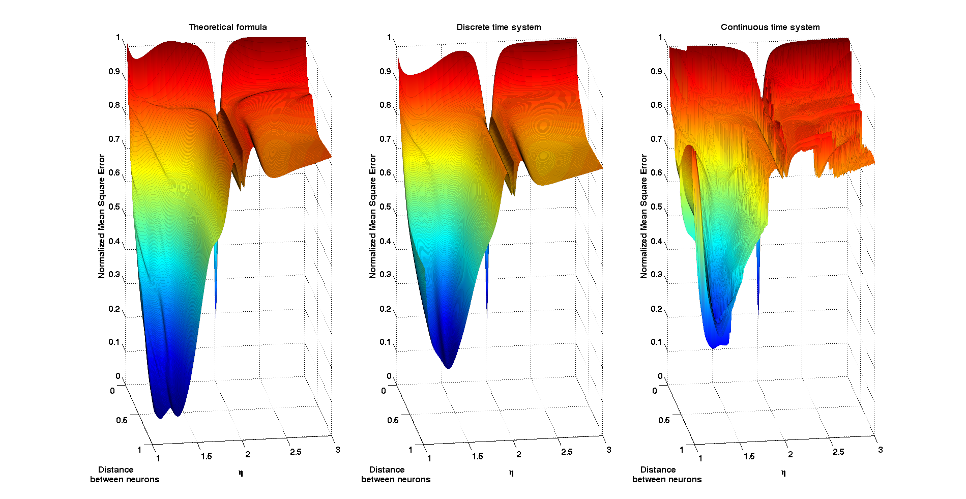
Figure 3: Error surfaces exhibited by a Mackey-Glass kernel based reservoir computer in a 6-lag quadratic memory task, as a function of the distance between neurons and the parameter $\eta$. The points in the surfaces of the middle and right panels are the result of Monte Carlo evaluations of the NMSE exhibited by the discrete and continuous time TDRs, respectively. The left panel was constructed using the formula (13) that is obtained as a result of modeling the reservoir with an approximating VAR(1) model.

In order to show that these statements are robust with respect to the choice of task and varying parameters, we have carried out a similar experiment with a RC in which we fix the feedback gain $\eta_{0}=1.0781$ and we vary the input gain $\gamma$ and the distance between neurons $d$. The quadratic memory task is reduced this time to 3-lags. We emphasize that in this setup the stable operation point is always the same and equal to $(\eta_{0}-1)^{1/2}$. Figure 4 shows how the performance of the memory capacity estimate (13) at the time of capturing the optimal parameter region is in this situation comparable to the results obtained for the 6-lag quadratic memory task represented in Figure 3. We also point out that in this case there is a lower variability of the performance which, in our opinion, has to do with the fact that modifying the parameter $\gamma$ adjusts the input gain but leaves unchanged the operation point. Additionally, the moderate difficulty of the task makes possible attaining lower optimal error rates with the same number of neurons. In order to ensure the robustness of these results with respect to the choice of nonlinear kernel, we have included in the Supplementary Material section the results of a similar experiment carried out using the Ikeda prescription.

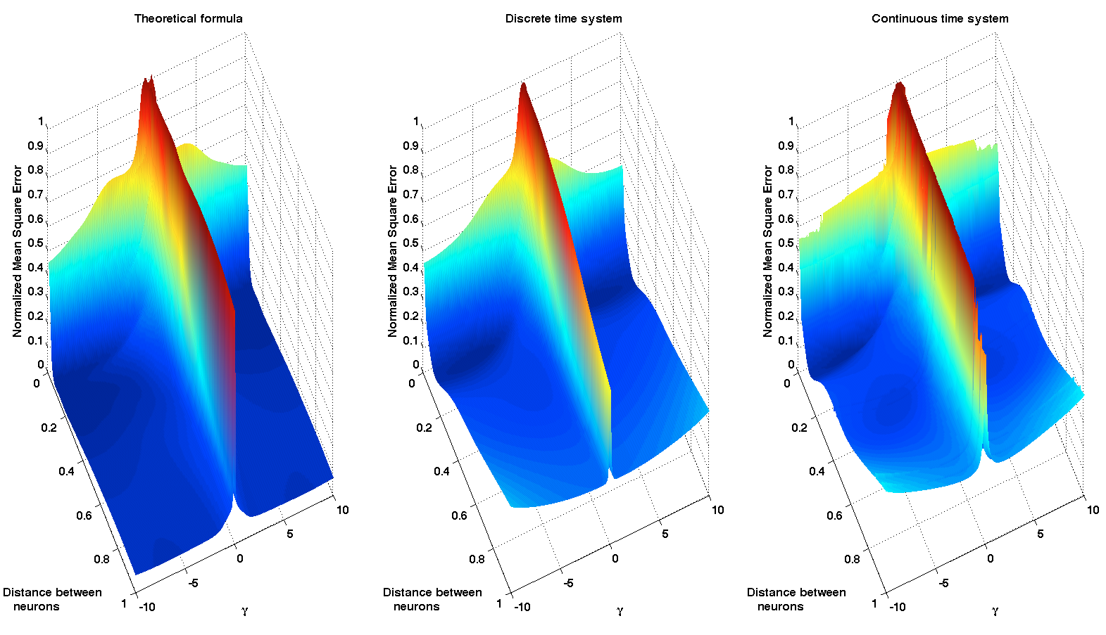
Figure 4: Error surfaces exhibited by a Mackey-Glass kernel based reservoir computer in a 3-lag quadratic memory task, as a function of the distance between neurons and the parameter $\gamma$. The points in the surfaces of the middle and right panels are the result of Monte Carlo evaluations of the NMSE exhibited by the discrete and continuous time TDRs, respectively. The left panel was constructed using the formula (13) that is obtained as a result of modeling the reservoir with an approximating VAR(1) model.

Once the adequacy of the memory capacity evaluation formula (13) has been established, we can use this result to investigate the influence of other architecture parameters in the reservoir performance. In Figure 5 we depict the results of an experiment where we study the influence of the choice of input mask ${\bf c}$ in the performance of a Mackey-Glass kernel based reservoir in a 3-lag quadratic memory task. The figure shows, for each number of neurons, the performance obtained by a RC in which the reservoir parameters $\boldsymbol{\theta}$ and the input mask ${\bf c}$ have been chosen so that the memory capacity $C_{H}(\boldsymbol{\theta},{\bf c},\lambda)$ in (13) is maximized; we have subsequently kept the optimal parameters $\boldsymbol{\theta}$ and we have randomly constructed one thousand input masks ${\bf c}$ with entries belonging to the interval $[-3,3]$. The box plots in Figure 5 give an idea of the distribution of the degraded performances with respect to the optimal mask for different numbers of virtual neurons.

Figure 5: Influence of the mask optimization on the reservoir performance in the 3-lag quadratic memory task. The red line links the points that indicate the error committed by a RC with optimized parameters and mask. The box plots give information about the distribution of performances obtained with 1,000 input masks randomly picked (only reservoir parameters have been optimized). As it is customary, on each box, the central mark is the median and the edges of the box are the 25th and 75th percentiles ($q_{1}$ and $q_{3}$, respectively). The whiskers extend to the most extreme data points not considered outliers and outliers are plotted individually using red crosses. Points are drawn as outliers if they are larger than $q_{3}+1.5(q_{3}Ðq_{1})$ or smaller than $q_{1}-1.5(q_{3}-q_{1})$. The blue line links the points that indicate the mean NMSE committed when using the 1,000 different randomly picked masks.

In conclusion, the construction of approximating models for the reservoir as well as the availability of performance evaluation formulas like (13) based on it, constitute extremely valuable analytical tools whose existence should prove very beneficial in the fast and efficient extension and customization of RC type techniques to tasks far more sophisticated than the ones we considered in this paper. This specific point is the subject of ongoing research on which we will report in a forthcoming publication.

Acknowledgments: We acknowledge partial financial support of the Région de Franche-Comté (Convention 2013C-5493), the European project PHOCUS (FP7 Grant No. 240763), the Labex ACTION program (Contract No. ANR-11-LABX-01-01), and Deployment S.L. LG acknowledges financial support from the Faculty for the Future Program of the Schlumberger Foundation.

Supplementary material for the paper “Optimal nonlinear information processing capacity in delay-based reservoir computers”

Appendix A Notation

Column vectors are denoted by bold lower or upper case symbol like $\mathbf{v}$ or $\mathbf{V}$. We write $\mathbf{v}^{\top}$ to indicate the transpose of $\mathbf{v}$. Given a vector $\mathbf{v}\in\mathbb{R}^{n}$, we denote its entries by $v_{i}$, with $i\in\left\{1,\dots,n\right\}$; we also write $\mathbf{v}=(v_{i})_{i\in\left\{1,\dots,n\right\}}$. The symbols $\mathbf{i}_{n}$ and $\mathbf{0}_{n}$ stand for the vectors of length $n$ consisting of zeros and ones, respectively.

We denote by $\mathbb{M}_{n,m}$ the space of real $n\times m$ matrices with $m,n\in\mathbb{N}$. When $n=m$, we use the symbol $\mathbb{M}_{n}$ to refer to the space of square matrices of order $n$. Given a matrix $A\in\mathbb{M}_{n,m}$, we denote its components by $A_{ij}$ and we write $A=(A_{ij})$, with $i\in\left\{1,\dots,n\right\}$, $j\in\left\{1,\dots m\right\}$. We use $\mathbb{S}_{n}$ to indicate the subspace $\mathbb{S}_{n}\subset\mathbb{M}_{n}$ of symmetric matrices, that is, $\mathbb{S}_{n}=\left\{A\in\mathbb{M}_{n}\mid A^{\top}=A\right\}$. Given a matrix $A\in\mathbb{M}_{n,m}$, the maximum row sum matrix norm is defined as $|||A|||_{\infty}=\max_{1\leq i\leq n}\sum^{m}_{j=1}|A_{ij}|$. The symbol $\otimes$ stands for the Kronecker matrix product.

We use ${C}^{r}([a,b],\mathbb{R})$, $r\geq 0$, to denote the Banach space of the $r$-times continuously differentiable real valued maps defined on the interval $[a,b]$ with the topology of the uniform convergence; given a function $g\in{C}^{r}([a,b],\mathbb{R})$ when $r\geq 1$. We designate the $l_{\infty}$-norm of an element $\phi\in{C}([a,b],\mathbb{R})$ by $||\phi||_{\infty}=\sup_{\theta\in\left[a,b\right]}|\phi(\theta)|$.

The symbols ${\rm E}[\cdot]$, ${\rm var}(\cdot)$, and ${\rm Cov}(\cdot,\cdot)$ denote the mathematical expectation, the variance, and the covariance, respectively.

Appendix B The reservoir map and the connectivity matrix

The reservoir map $F:\mathbb{R}^{N}\times\mathbb{R}^{N}\times\mathbb{R}^{K}\longrightarrow\mathbb{R}^{N}$ introduced in (4) is uniquely determined by the recursions (3) obtained out of the Euler discretization of the time-delay differential equation (TDDE)

$$\dot{x}(t)=-x(t)+f(x(t-\tau),I(t),\boldsymbol{\theta}),$$ (B.1)

and organized in neuron layers parametrized by $t\in\mathbb{Z}$. The reservoir map is obtained by using (3) in order to write down the neuron values of the layer for time $t$ in terms of those for time $t-1$ and the current input signal value. More specifically:

$$\left\{\begin{array}[]{rcl}x_{1}(t)&=&e^{-\xi}x_{N}(t-1)+(1-e^{-\xi})f(x_{1}(t-1),I_{1}(t),\boldsymbol{\theta}),\\ x_{2}(t)&=&e^{-2\xi}x_{N}(t-1)+(1-e^{-\xi})\left\{e^{-\xi}f(x_{1}(t-1),I_{1}(t),\boldsymbol{\theta})+f(x_{2}(t-1),I_{2}(t),\boldsymbol{\theta})\right\},\\ &\vdots&\\ x_{N}(t)&=&e^{-N\xi}x_{N}(t-1)+(1-e^{-\xi})\sum^{N-1}_{j=0}e^{-j\xi}f(x_{N-j}(t-1),I_{N-j}(t),\boldsymbol{\theta}),\end{array}\right.$$ (B.2)

which corresponds to a description of the form

$$\mathbf{x}(t)=F(\mathbf{x}(t-1),\mathbf{I}(t),\boldsymbol{\theta}),$$ (B.3)

that uniquely determines the reservoir map $F:\mathbb{R}^{N}\times\mathbb{R}^{N}\times\mathbb{R}^{K}\longrightarrow\mathbb{R}^{N}$.

Let $x_{0}\in\mathbb{R}$ and $\mathbf{x}_{0}:=x_{0}\mathbf{i}_{N}\in\mathbb{R}^{N}$. Let $D_{\mathbf{x}}F(\mathbf{x}_{0},{\bf 0}_{N},\boldsymbol{\theta})$ be the partial derivative of $F$ with respect to the first argument computed at the point $(\mathbf{x}_{0},{\bf 0}_{N},\boldsymbol{\theta})$. We will refer to $A(\mathbf{x}_{0},\boldsymbol{\theta}):=D_{\mathbf{x}}F(\mathbf{x}_{0},{\bf 0}_{N},\boldsymbol{\theta})$ as the connectivity matrix of the reservoir at the point $\mathbf{x}_{0}$. It is easy to show that $A(\mathbf{x}_{0},\boldsymbol{\theta})$ has the following explicit form

$$A(\mathbf{x}_{0},\boldsymbol{\theta}):=D_{\mathbf{x}}F(\mathbf{x}_{0},{\bf 0}_{N},\boldsymbol{\theta})={\small\left(\begin{array}[]{cccccc}\Phi&0&\ldots&0&{e^{-\xi}{}}\\ {e^{-\xi}}\Phi&\Phi&\ldots&0&{e^{-2\xi}{}}\\ e^{-2\xi}\Phi&e^{-\xi}\Phi&\ldots&0&{e^{-3\xi}{}}\\ \vdots&\vdots&\ddots&\vdots&\vdots\\ e^{-(N-1)\xi}\Phi&e^{-(N-2)\xi}\Phi&\ldots&{e^{-\xi}}{}\Phi&\Phi+{e^{-N\xi}{}}\end{array}\right)},$$ (B.9)

where $\Phi:=(1-e^{-\xi})\partial_{x}f(x_{0},0,\boldsymbol{\theta})$ and $\partial_{x}f(x_{0},0,\boldsymbol{\theta})$ is the first derivative of the nonlinear kernel $f$ in (B.1) with respect to the first argument and computed at the point $(x_{0},0,\boldsymbol{\theta})$. We will also use the symbol $f^{\prime}_{x_{0}}$ to denote $\partial_{x}f(x_{0},0,\boldsymbol{\theta})$.

Appendix C The approximating vector autoregressive system and information processing capacity estimations

The goal of this appendix is providing details on the construction of the approximating VAR(1) model for the TDR obtained after a partial linearization of the reservoir map on the dynamical variables and respecting the nonlinearity on the input signal. Let $x_{0}\in\mathbb{R}$ and $\mathbf{x}_{0}:=x_{0}\mathbf{i}_{N}\in\mathbb{R}^{N}$ be an equilibrium of (B.1) and a fixed point of (B.3), respectively (see Proposition D.9). These solutions are chosen with respect to the autonomous regime, that is, we set $I(t)=0$ in the time-delay differential equation (B.1) and $\mathbf{I}(t)={\bf 0}_{N}$ in the associated recursion (B.3). In practice, we choose stable solutions; Appendix D contains conditions that ensure this dynamical feature.

The VAR model setup and the construction of the approximating VAR system. The vector autoregressive (VAR) model is of much use in multivariate time series analysis and is a natural extension of the univariate linear autoregressive (AR) model. See [Lutk 05] for an extensive introduction to multivariate time series methods and the details on the VAR processes. The $N$-dimensional VAR(1) process (VAR model of order 1) is defined in mean-adjusted form as the solution to the recursions

$$\mathbf{x}(t)-\boldsymbol{\mu}_{x}=A(\mathbf{x}(t-1)-\boldsymbol{\mu}_{x})+\boldsymbol{\epsilon}(t),\enspace t=0,\pm 1,\pm 2,\ldots$$ (C.1)

where $\mathbf{x}(t)=(x_{1}(t),\ldots,x_{N}(t))^{\top}\in\mathbb{R}^{N}$ is a random vector, $A\in\mathbb{M}_{N}$ is a fixed coefficient matrix, $\boldsymbol{\mu}_{x}\in\mathbb{R}^{N}$, and $\boldsymbol{\epsilon}(t)=(\epsilon_{1}(t),\ldots,\epsilon_{N}(t))^{\top}\in\mathbb{R}^{N}$ is such that $\left\{\boldsymbol{\epsilon}(t)\right\}\sim{\rm WN}({\bf 0}_{N},\Sigma_{\epsilon})$ is a $N$-dimensional white noise (stochastic process that presents no autocorrelation) or innovation process with mean ${\bf 0}_{N}$ and covariance matrix $\Sigma_{\epsilon}\in\mathbb{S}_{N}$. We are particularly interested in stable VAR models, that is, models of the type (C.1) where the autoregression matrix $A$ is chosen such that

$$\det\left(\mathbb{I}_{N}-Az\right)\neq 0\quad\mbox{for all $z\in\mathbb{C}$ such that $|z|\leq 1$}.$$ (C.2)

It can be proved (see Proposition 2.1 in [Lutk 05]) that stable models have a unique second order stationary solution $\{\mathbf{x}(t)\}_{t\in\mathbb{Z}}$ for which $\boldsymbol{\mu}_{x}={\rm E}[\mathbf{x}(t)]$ and the autocovariance function

$$\Gamma(k):={\rm E}\left[\left(\mathbf{x}(t)-\boldsymbol{\mu}_{{x}}\right)\left(\mathbf{x}(t-k)-\boldsymbol{\mu}_{{x}}\right)^{\top}\right],\enspace k\in\mathbb{Z}$$

is time independent.

Let now $\mathbf{x}_{0}=x_{0}\mathbf{i}_{N}\in\mathbb{R}^{N}$ be the stable fixed point of the reservoir map (B.3) in autonomous regime, that is, $F({\bf x}_{0},{\bf 0}_{N},\boldsymbol{\theta})={\bf x}_{0}$. We now approximate (B.3) by its partial linearization at $\mathbf{x}_{0}$ with respect to the delayed self feedback and by the $R$th-order Taylor series expansion on the variable that determines the input signal injection. We obtain the following expression:

$$\mathbf{x}(t)=F(\mathbf{x}_{0},{\bf 0}_{N},\boldsymbol{\theta})+D_{\mathbf{x}}F(\mathbf{x}_{0},{\bf 0}_{N},\boldsymbol{\theta})(\mathbf{x}(t-1)-\mathbf{x}_{0})+\boldsymbol{\varepsilon}(t),$$ (C.3)

where $D_{\mathbf{x}}F(\mathbf{x}_{0},{\bf 0}_{N},\boldsymbol{\theta})$ is the first derivative of $F$ with respect to its first argument, computed at the point $(\mathbf{x}_{0},{\bf 0}_{N},\boldsymbol{\theta})$. We recall that $D_{\mathbf{x}}F(\mathbf{x}_{0},{\bf 0}_{N},\boldsymbol{\theta})=A(\mathbf{x}_{0},\boldsymbol{\theta})$ is the connectivity matrix introduced in (B.9). Additionally, $\boldsymbol{\varepsilon}(t)$ in (C.3) is obtained out of the Taylor series expansion of $F(\mathbf{x}(t),\mathbf{I}(t),\boldsymbol{\theta})$ in (B.2) on $\mathbf{I}(t)$ up to some fixed order $R\in\mathbb{N}$ and is given by

$$\boldsymbol{\varepsilon}(t)=(1-{e}^{-\xi})(q_{R}\left(z(t),c_{1}\right),q_{R}\left(z(t),c_{1},c_{2}\right),\dots,q_{R}\left(z(t),c_{1},\dots,c_{N}\right))^{\top},$$ (C.4)

with

$$q_{R}\left(z(t),c_{1},\dots,c_{r}\right):=\sum^{R}_{i=1}\dfrac{z(t)^{i}}{i!}(\partial_{{I}}^{(i)}f)({x}_{0},0,\boldsymbol{\theta}){\sum^{r}_{j=1}{e}^{-(r-j)\xi}c_{j}^{i}},$$ (C.5)

where $c_{i}$, $i\in\left\{1,\ldots,N\right\}$ are the entries of the input mask ${\bf c}\in\mathbb{R}^{N}$ and $(\partial_{{I}}^{(i)}f)({x}_{0},0,\boldsymbol{\theta})$ is the $i$th order partial derivative of the nonlinear reservoir kernel $f$ in (B.1) with respect to the second argument $I(t)$ computed at the point $({x}_{0},0,\boldsymbol{\theta})$.

If we now use as input signal ${z}(t)$ independent and identically distributed random variables with mean $0$ and variance $\sigma_{z}^{2}$, that is, $\left\{{z}(t)\right\}_{t\in\mathbb{Z}}\sim{\rm IID}(0,\sigma_{z}^{2})$, then the recursion (C.3) makes the reservoir layer dynamics $\{\mathbf{x}(t)\}_{t\in\mathbb{Z}}$ into a discrete time random process that, as we show in what follows, is the solution of a $N$-dimensional VAR(1) model. Indeed, it is easy to see that the assumption $\left\{{z}(t)\right\}_{t\in\mathbb{Z}}\sim{\rm IID}(0,\sigma_{z}^{2})$ implies that $\left\{\mathbf{I}(t)\right\}_{t\in\mathbb{Z}}\sim{\rm IID}({\bf 0}_{N},\Sigma_{I})$, with $\Sigma_{I}:=\sigma_{z}^{2}{\bf c}^{\top}{\bf c}$, and that $\{\boldsymbol{\varepsilon}(t)\}_{t\in\mathbb{Z}}$ is a family of $N$-dimensional independent and identically distributed random variables with mean $\boldsymbol{\mu}_{{\varepsilon}}$ and covariance matrix $\Sigma_{{\varepsilon}}$ given by the following expression:

$$\boldsymbol{\mu}_{{\varepsilon}}={\rm E}\left[\boldsymbol{\varepsilon}(t)\right]=(1-{e}^{-\xi})\left(q_{R}\left(\mu_{{z}},c_{1}\right),q_{R}\left(\mu_{{z}},c_{1},c_{2}\right),\ldots,q_{R}\left(\mu_{{z}},c_{1},\dots,c_{N}\right)\right)^{\top},$$ (C.6)

where the polynomial $q_{R}$ is the same as in (C.5) and where we use the convention that the powers $\mu_{{z}}^{i}:={\rm E}\left[z(t)^{i}\right]$, for any $i\in\left\{1,\dots,R\right\}$. For example, if the variables $z(t)$ are normal, that is, $\left\{{z}(t)\right\}_{t\in\mathbb{Z}}\sim{\rm IN}(0,\sigma_{z}^{2})$, then

$$\mu_{{z}}^{i}:={\rm E}\left[z(t)^{i}\right]=\left\{\begin{array}[]{cl}\dfrac{2l!}{2^{l}l!}\sigma_{z}^{2l}&{\rm when}\enspace i=2l,\quad l\in\mathbb{N},\\ &\\ 0&{\rm otherwise}.\end{array}\right.$$ (C.7)

Additionally, $\Sigma_{{\varepsilon}}:={\rm E}\left[(\boldsymbol{\varepsilon}(t)-\boldsymbol{\mu}_{{\varepsilon}})(\boldsymbol{\varepsilon}(t)-\boldsymbol{\mu}_{{\varepsilon}})^{\top}\right]$ has entries determined by the relation:

$$(\Sigma_{{\varepsilon}})_{ij}=(1-{e}^{-\xi})^{2}((q_{R}(\cdot,c_{1},\dots,c_{i})\cdot q_{R}(\cdot,c_{1},\dots,c_{j}))(\mu_{{z}})-q_{R}(\mu_{{z}},c_{1},\dots,c_{i})q_{R}(\mu_{{z}},c_{1},\dots,c_{j})),$$

where the first summand stands for the multiplication of the polynomials $q_{R}(\cdot,c_{1},\dots,c_{i})$ and $q_{R}(\cdot,c_{1},\dots,c_{j})$ and the subsequent evaluation of the resulting polynomial at $\mu_{z}$, and the second one is made out of the multiplication of the evaluation of the two polynomials.

With these observations it is clear that we can consider (C.3) as a VAR(1) model driven by the independent noise $\{\boldsymbol{\varepsilon}(t)\}_{t\in\mathbb{Z}}$. If the nonlinear kernel $f$ satisfies the generic condition that the polynomial in $z$ given by $\det\left(\mathbb{I}_{N}-A(\mathbf{x}_{0},\boldsymbol{\theta})z\right)$, does not have roots in and on the complex unit circle, then (C.3) has a unique second order stationary solution $\{\mathbf{x}(t)\}_{t\in\mathbb{Z}}$ with time-independent mean

$$\boldsymbol{\mu}_{{x}}={\rm E}\left[\mathbf{x}(t)\right]=(I_{N}-A(\mathbf{x}_{0},\boldsymbol{\theta}))^{-1}(F(\mathbf{x}_{0},{\bf 0}_{N},\boldsymbol{\theta})-A(\mathbf{x}_{0},\boldsymbol{\theta})\mathbf{x}_{0}+\boldsymbol{\mu}_{{\varepsilon}}).$$ (C.8)

that can be used to rewrite (C.3) in mean-adjusted form

$$\mathbf{x}(t)-\boldsymbol{\mu}_{{x}}=A(\mathbf{x}_{0},\boldsymbol{\theta})(\mathbf{x}(t-1)-\boldsymbol{\mu}_{{x}})+(\boldsymbol{\varepsilon}(t)-\boldsymbol{\mu}_{{\varepsilon}}).$$ (C.9)

In the presence of stationarity we can recursively compute the time independent autocovariance function $\Gamma(k):={\rm E}\left[\left(\mathbf{x}(t)-\boldsymbol{\mu}_{{x}}\right)\left(\mathbf{x}(t-k)-\boldsymbol{\mu}_{{x}}\right)^{\top}\right]$ at lag $k\in\mathbb{Z}$ by using the Yule-Walker equations [Lutk 05]. Indeed, $\Gamma(0)$ is given by the vectorized equality:

$${\rm vec}(\Gamma(0))=\left(\mathbb{I}_{N^{2}}-A(\mathbf{x}_{0},\boldsymbol{\theta})\otimes A(\mathbf{x}_{0},\boldsymbol{\theta})\right)^{-1}{\rm vec}(\Sigma_{{\varepsilon}}),$$ (C.10)

which determines the higher order autocovariances via the relation

$$\Gamma(k)=A(\mathbf{x}_{0},\boldsymbol{\theta})\Gamma(k-1),$$ (C.11)

and the identity $\Gamma(-k)=\Gamma(k)^{\top}$.

The nonlinear memory capacity estimations. We now concentrate on the computation of the quantitative measures of the reservoir performance introduced in the paper. In particular, we will provide details on the computation of the nonlinear memory capacity formula in (13). Recall that a $h$-lag memory task is determined by a function $H:\mathbb{R}^{h+1}\rightarrow\mathbb{R}$ (in general nonlinear) that is used to generate a one-dimensional signal $y(t):=H(z(t),z(t-1),\ldots,z(t-h))$ out of the reservoir input $\left\{z(t)\right\}_{t\in\mathbb{Z}}$.

Consider now a TDR computer with $N$ neurons. The optimal linear readout ${\mathbf{W}}_{{\rm out}}$ adapted to the memory task $H$ is given by the solution of a ridge (or Tikhonov [Tikh 43]) linear regression problem with regularization parameter $\lambda\in\mathbb{R}$ (usually tuned during the training phase via cross-validation) in which the covariates are the neuron values corresponding to the reservoir output and the explained variables are the values $\{y(t)\}$ of the memory task function. More explicitly, ${\mathbf{W}}_{{\rm out}}$ is given by the solution of the following optimization problem

$$({\mathbf{W}}_{{\rm out}},a_{\rm out}):=\mathop{\rm arg\,min}_{{\mathbf{W}}\in\mathbb{R}^{N},a\in\mathbb{R}}\left({\rm E}\left[({\mathbf{W}}^{\top}\cdot{\bf x}(t)+a-{y}(t))^{2}\right]+\lambda\|{\mathbf{W}}\|^{2}\right),$$ (C.12)

where the expectation is taken thinking of $y_{t}$ and $\mathbf{x}(t)$ as random variables due to the stochastic nature of the input signal $\left\{z(t)\right\}_{t\in\mathbb{Z}}$ and hence that of the $\left\{\mathbf{I}(t)\right\}_{t\in\mathbb{Z}}$. In order to obtain the explicit solution of (C.12), we first define $g({\mathbf{W}},a):={\rm E}\left[({\mathbf{W}}^{\top}\cdot{\bf x}(t)+a-{y}(t))^{2}\right]+\lambda\|{\mathbf{W}}\|^{2}$ and set

$$\dfrac{\partial g({\mathbf{W}},a)}{\partial w_{i}}= 2\left[\sum^{N}_{j=1}w_{j}{\rm Cov}(x_{j}(t),x_{i}(t))-{\rm Cov}(y(t),x_{i}(t))+\lambda w_{i}\right]=0,\enspace i\in\left\{1,\ldots,N\right\},$$

$$\dfrac{\partial g({\mathbf{W}},a)}{\partial a}= 2\left[a+{\mathbf{W}}^{\top}{\rm E}\left[\mathbf{x}(t)\right]-{\rm E}\left[y(t)\right]\right]=0,$$

or, equivalently,

$$({\rm Cov}(\mathbf{x}(t),\mathbf{x}(t))+\lambda I_{N}){\mathbf{W}}-{\rm Cov}(y(t),\mathbf{x}(t))=0,$$

$$a+{\mathbf{W}}^{\top}{\rm E}\left[\mathbf{x}(t)\right]-{\rm E}\left[y(t)\right]=0.$$

These equations yield the pair $({\mathbf{W}}_{\rm out},a_{\rm out})$ that minimizes $g({\mathbf{W}},a)$. We now use the fact that $\{\mathbf{x}(t)\}_{t\in\mathbb{Z}}$ is the unique stationary solution of VAR(1) approximating system (C.9) for the TDR (C.9) and hence obtain

$${\mathbf{W}}_{\rm out}= (\Gamma(0)+\lambda I_{N})^{-1}{\rm Cov}(y(t),\mathbf{x}(t)),$$ (C.13)

$$a_{\rm out}= {\rm E}\left[y(t)\right]-{\mathbf{W}}_{\rm out}^{\top}\boldsymbol{\mu}_{x},$$ (C.14)

where $\boldsymbol{\mu}_{x}$ is provided in (C.8), $\Gamma(0)\in\mathbb{S}_{N}$ is determined by the generalized Yule-Walker equations in (C.10) and ${\rm Cov}(y(t),\mathbf{x}(t))$ is a vector in $\mathbb{R}^{N}$ that has to be determined for every specific memory task $H$. Additionally, it is easy to verify that the error committed by the reservoir when using the optimal readout is

$${\rm E}\left[\left({\mathbf{W}}_{{\rm out}}^{\top}\cdot{\bf x}(t)+a_{{\rm out}}-{y}(t)\right)^{2}\right]={\mathbf{W}}_{{\rm out}}^{\top}\Gamma(0){\mathbf{W}}_{{\rm out}}+{\rm var}\left(y(t)\right)-2{\mathbf{W}}_{{\rm out}}^{\top}{\rm Cov}(y(t),\mathbf{x}(t))$$

$$={\rm var}\left(y(t)\right)-{\mathbf{W}}_{{\rm out}}^{\top}(\Gamma(0)+2\lambda\mathbb{I}_{N}){\mathbf{W}}_{{\rm out}}$$

$$={\rm var}\left(y(t)\right)-{\rm Cov}(y(t),\mathbf{x}(t))^{\top}(\Gamma(0)+\lambda\mathbb{I}_{N})^{-1}(\Gamma(0)+2\lambda\mathbb{I}_{N})(\Gamma(0)+\lambda\mathbb{I}_{N})^{-1}{\rm Cov}(y(t),\mathbf{x}(t)).$$ (C.15)

The $H$-memory capacity $C_{H}(\boldsymbol{\theta},{\bf c},\lambda)$ of a reservoir computer constructed using a nonlinear kernel $f$ with parameters $\boldsymbol{\theta}$, an input mask ${\bf c}$, and regularizing ridge parameter $\lambda$, is defined as one minus the normalized mean square error committed at the time of accomplishing the memory task $H$. Expression (C) shows that when the RC is approximated by the VAR(1) model (C.9), the corresponding $H$-memory capacity can be approximated by

$$C_{H}(\boldsymbol{\theta},{\bf c},\lambda)=\frac{{\rm Cov}(y(t),\mathbf{x}(t))^{\top}(\Gamma(0)+\lambda\mathbb{I}_{N})^{-1}(\Gamma(0)+2\lambda\mathbb{I}_{N})(\Gamma(0)+\lambda\mathbb{I}_{N})^{-1}{\rm Cov}(y(t),\mathbf{x}(t))}{{\rm var}\left(y(t)\right)}$$ (C.16)

Since the normalized error coming from the expression (C) is clearly bounded between zero and one, it is also clear that:

$$0\leq C_{H}(\boldsymbol{\theta},{\bf c},\lambda)\leq 1.$$

We emphasize that in order to evaluate (C.16) for a specific memory task, only ${\rm Cov}(y(t),\mathbf{x}(t))$ and ${\rm var}\left(y(t)\right)$ need to be computed since the autocovariance $\Gamma(0)$ is fully determined by (C.10) once the reservoir and the equilibrium $\mathbf{x}_{0}$ around which we operate have been chosen.

Once a specific reservoir and task $H$ have been fixed, the capacity function $C_{H}(\boldsymbol{\theta},{\bf c},\lambda)$ can be explicitly written down and it can hence be used to find reservoir parameters ${\boldsymbol{\theta}}_{{\rm opt}}$ and an input mask ${\bf c}_{\rm opt}$ that maximize it, by solving the optimization problem

$$({\boldsymbol{\theta}}_{{\rm opt}},{\bf c}_{\rm opt}):=\mathop{\rm arg\,max}_{{\boldsymbol{\theta}}\in\mathbb{R}^{K},{\bf c}\in\mathbb{R}^{N}}C_{H}(\boldsymbol{\theta},{\bf c},\lambda).$$ (C.17)

Two specific memory tasks. In the following paragraphs we spell out the computation of ${\rm Cov}(y(t),\mathbf{x}(t))$ and ${\rm var}\left(y(t)\right)$ necessary to evaluate the memory capacity formula (C.16) for the two most basic memory tasks, namely, the linear and the quadratic ones.

(i)

The $h$-lag linear memory task. The linear memory task is determined by the linear task functions $H:\mathbb{R}^{h+1}\rightarrow\mathbb{R}$ that we now describe. First, let ${\bf z}^{h}(t):=\left(z(t),z(t-1),\ldots,z(t-h)\right)^{\top}$ and let $\mathbf{L}\in\mathbb{R}^{h+1}$. We then set $H({\bf z}^{h}(t)):=\mathbf{L}^{\top}{\bf z}^{h}(t)$. In order to evaluate the $h$-lag memory capacity using formula (C.16), we need to evaluate ${\rm var}\left(y(t)\right)$ and ${\rm Cov}(y(t),\mathbf{x}(t))$ with $y(t):=H({\bf z}^{h}(t))$.

First, since $\left\{z(t)\right\}_{t\in\mathbb{Z}}\sim{\rm IID}(0,\sigma_{z}^{2})$, we then immediately obtain that

$${\rm var}({y}(t))=\sigma_{{z}}^{2}||\mathbf{L}||^{2}.$$ (C.18)

Next, we use the so called MA($\infty$)-representation of the VAR(1) in (C.9), namely,

$$(\mathbf{x}(t)-\boldsymbol{\mu}_{{x}})=\sum^{\infty}_{i=0}\Psi_{i}\boldsymbol{\rho}({t-i}),$$ (C.19)

with $\boldsymbol{\mu}_{{x}}$ as in (C.8), $\boldsymbol{\rho}(t):=\boldsymbol{\varepsilon}(t)-\boldsymbol{\mu}_{{\varepsilon}}$, $\boldsymbol{\mu}_{{\varepsilon}}$ defined in (C.6), $\Psi_{i}=A(\mathbf{x}_{0},\boldsymbol{\theta})^{i}$, and $A(\mathbf{x}_{0},\boldsymbol{\theta})$ the connectivity matrix of the discretized nonlinear TDR provided in (B.9). Using (C.19), we compute

$${\rm Cov}({y}(t),x_{i}(t))={\rm Cov}(\mathbf{L}^{\top}\mathbf{z}^{h}(t),x_{i}(t))=\sum^{h+1}_{j=1}L_{j}{\rm Cov}(z(t-j+1),x_{i}(t))$$

$$=\sum^{h+1}_{j=1}\sum^{\infty}_{k=0}\sum^{N}_{r=1}L_{j}(A(\mathbf{x}_{0},\boldsymbol{\theta})^{k})_{ir}{\rm E}\left[z({t-j+1})\rho_{r}({t-k})\right]$$

$$=\sum^{h+1}_{j=1}\sum^{N}_{r=1}L_{j}(A(\mathbf{x}_{0},\boldsymbol{\theta})^{j-1})_{ir}{\rm E}\left[z({t})(\varepsilon_{r}({t})-z(t)(\boldsymbol{\mu}_{\varepsilon})_{r}\right],\enspace{\rm with}\enspace i\in\{1,\ldots,N\},$$ (C.20)

which immediately yields that

$${\rm Cov}({y}(t),x_{i}(t))=(1-{e}^{-\xi})\sum^{h+1}_{j=1}\sum^{N}_{r=1}L_{j}(A(\mathbf{x}_{0},\boldsymbol{\theta})^{j-1})_{ir}p_{R}(\mu_{z},c_{1},\dots,c_{r}),\enspace{\rm with}\enspace i\in\{1,\ldots,N\},$$ (C.21)

where the polynomial $p_{R}$ on the variable $x$ is defined by $p_{R}(x,c_{1},\dots,c_{r}):=x\cdot q_{R}(x,c_{1},\dots,c_{r})$ and its evaluation follows the same convention as in (C.6). The expressions (C.18) and (C.21) can be readily substituted in (C.16) in order to obtain an explicit expression for capacity $C_{H}(\boldsymbol{\theta},{\bf c},\lambda)$ associated to the $h$-lag linear memory task as a function of the reservoir parameters $\boldsymbol{\theta}$ and the input mask ${\bf c}$. This expression can be subsequently treated as in (C.17) in order to determine optimal architecture parameters for this particular task.

(ii)

The $h$-lag quadratic memory task. In this case we use a quadratic task function $H:\mathbb{R}^{h+1}\rightarrow\mathbb{R}$ of the form

$$H({\bf z}^{h}(t)):=\mathbf{z}^{h}(t)^{\top}Q\mathbf{z}^{h}(t)=\sum^{h+1}_{i=1}\sum^{h+1}_{j=1}Q_{ij}z({t-i+1})z({t-j+1}),$$ (C.22)

for some symmetric matrix $Q\in\mathbb{S}_{h+1}$. Analogously to the linear task case, in order to evaluate the memory capacity associated to $H$, we have to derive explicit expressions for ${\rm var}\left(y(t)\right)$ and ${\rm Cov}(y(t),\mathbf{x}(t))$ with $y(t):=H({\bf z}^{h}(t))$. The same computations as in the case of the linear task apply. First, if $\left\{z(t)\right\}_{t\in\mathbb{Z}}\sim{\rm IID}(0,\sigma_{z}^{2})$, we can immediately write

$${\rm E}\left[{y}(t)\right]=\sigma_{{z}}^{2}{\rm tr}(Q),$$ (C.23)

and

$${\rm E}\left[{y}(t)^{2}\right] = \sum_{i=1}^{h+1}\sum_{j=1}^{h+1}\sum_{k=1}^{h+1}\sum_{l=1}^{h+1}{\rm E}\left[Q_{ij}Q_{kl}z(t-i+1)z(t-j+1)z(t-k+1)z(t-l+1)\right]$$ (C.24)

$$= \sum_{i=1}^{h+1}Q_{ii}^{2}{\rm E}\left[z(t-i+1)^{4}\right]+4\sum_{i=1}^{h+1}\sum_{j>i}^{h+1}Q_{ij}^{2}{\rm E}\left[z(t-i+1)^{2}z(t-j+1)^{2}\right]$$

$$+2\sum_{i=1}^{h+1}\sum_{j>i}^{h+1}Q_{ii}Q_{jj}{\rm E}\left[z(t-i+1)^{2}z(t-j+1)^{2}\right]$$

$$= \mu_{z}^{4}\sum_{i=1}^{h+1}Q_{ii}^{2}+4\sigma_{z}^{4}\sum_{i=1}^{h+1}\sum_{j>i}^{h+1}Q_{ij}^{2}+2\sigma_{z}^{4}\sum_{i=1}^{h+1}\sum_{j>i}^{h+1}Q_{ii}Q_{jj}.$$

Analogously, by (C.23),

$${\rm E}\left[{y}(t)\right]^{2}=\sigma_{{z}}^{4}{\rm tr}(Q)^{2}=\sigma_{{z}}^{4}\left(\sum_{i=1}^{h+1}Q_{ii}^{2}+2\sum_{i=1}^{h+1}\sum_{j>i}^{h+1}Q_{ii}Q_{jj}\right).$$ (C.26)

Hence, if we put together (C.24) and (C.26), we obtain

$${\rm var}({y}(t))={\rm E}\left[{y}(t)^{2}\right]-{\rm E}\left[{y}(t)\right]^{2}=(\mu_{z}^{4}-\sigma_{z}^{4})\sum_{i=1}^{h+1}Q_{ii}^{2}+4\sigma_{z}^{4}\sum_{i=1}^{h+1}\sum_{j>i}^{h+1}Q_{ij}^{2}.$$ (C.27)

Recall that for Gaussian variables, that is $\left\{z(t)\right\}_{t\in\mathbb{Z}}\sim{\rm IN}(0,\sigma_{z}^{2})$, we have that $\mu_{z}^{4}=3\sigma_{z}^{2}$, and hence in that case

$${\rm var}({y}(t))=2\sigma_{z}^{4}\left(\sum_{i=1}^{h+1}Q_{ii}^{2}+2\sum_{i=1}^{h+1}\sum_{j>i}^{h+1}Q_{ij}^{2}\right)=2\sigma_{z}^{4}\sum_{i=1}^{h+1}\sum_{j=1}^{h+1}Q_{ij}^{2}.$$ (C.28)

Regarding the computation of the covariance and analogously to the case of the linear $h$-lag memory task, we use the MA($\infty$) representation of the VAR(1) model of the TDR in (C.9) and write

$${\rm Cov}({y}(t),x_{i}(t))= \sum^{h+1}_{j=1}\sum^{h+1}_{k=1}\sum^{\infty}_{l=1}Q_{jk}{\rm E}\left[z({t-j+1})z({t-k+1})(A(\mathbf{x}_{0},\boldsymbol{\theta})^{l}\boldsymbol{\rho}({t-l}))_{i}\right]$$

$$= \sum^{\infty}_{l=0}\sum^{h+1}_{j=1}\sum^{h+1}_{k=1}\sum^{N}_{r=1}Q_{jk}(A(\mathbf{x}_{0},\boldsymbol{\theta})^{l})_{ir}\Big{\{}{\rm E}\left[z({t-j+1})z({t-k+1})\varepsilon_{r}({t-l})\right]$$

$$-(\boldsymbol{\mu}_{{\varepsilon}})_{r}{\rm E}\left[z({t-j+1})z({t-k+1})\right]\Big{\}},\enspace{\rm with}\enspace i\in\{1,\ldots,N\},$$

which leads to the following result:

$${\rm Cov}({y}(t),x_{i}(t))=(1-{e}^{-\xi})\sum^{h+1}_{j=1}\sum^{N}_{r=1}Q_{jj}(A(\mathbf{x}_{0},\boldsymbol{\theta})^{j-1})_{ir}(s_{R}(\mu_{{z}},c_{1},\dots,c_{r})-\sigma_{z}^{2}q_{R}(\mu_{z},c_{1},\dots,c_{r})),$$ (C.29)

with $i\in\{1,\ldots,N\}$. In this relation the polynomial $s_{R}$ on $x$ is defined as $s_{R}(x,c_{1},\dots,c_{r}):=x^{2}\cdot q_{R}(x,c_{1},\dots,c_{r})$ and is evaluated following the same convention as in (C.6) but taking $x^{2}$ instead of $x$.

Again, we conclude by noticing that the expressions (C.29) and (C.27) substituted in (C.16) provide an explicit formula for capacity $C_{H}(\boldsymbol{\theta},{\bf c},\lambda)$ associated to the $h$-lag quadratic memory task as a function of the reservoir parameters $\boldsymbol{\theta}$ and the input mask ${\bf c}$ and hence it can be readily used to solve the optimization problem in (C.17).

An observation that is worth to be pointed out is that only the diagonal elements in $Q$ intervene in the covariance (C.29) while all its entries are present in the variance (C.27). When these two quantities are substituted in the memory capacity formula (C.16) it can be seen that by choosing sufficiently high off-diagonal entries in $Q$, the capacity of the reservoir can be made arbitrarily small which shows a structural limitation of the architecture that we are considering that can only be fixed by using alternative signal feeding schemes.

Appendix D Equilibria of the continuous and the discrete time models for the TDR and their stability

As we already explained, the linearization of the reservoir map at a stable fixed point is at the core of the developments in this paper. That is why in this section we carry out a detailed study of the stability properties of the equilibria of the time-delay differential equation (B.1) and of the fixed points of its corresponding discrete-time approximation (B.3). More specifically, we provide sufficient stability conditions and we show that our results exhibit a remarkable consistence regardless of the use of the continuous or of the discrete time schemes.

D.1 Stationary solutions of time-delay differential equations and their stability

We start by recalling some basic facts about the properties of the solutions of the time-delay differential equations and their stability. Let $\tau\in\mathbb{R}^{+}$ be a fixed delay and consider a time-delay map

$$\begin{array}[]{ccccccc}X:&{C}^{1}([-\tau,0],\mathbb{R})\times\mathbb{R}&\longrightarrow&\mathbb{R}\\ &({\gamma},t)&\longmapsto&X(\gamma,t).\end{array}$$ (D.3)

Additionally, for any $t\in\mathbb{R}$ define the shift operator

$$\begin{array}[]{ccccccc}S_{t}:&{C}^{1}([-\tau+t,t],\mathbb{R})&\longrightarrow&{C}^{1}([-\tau,0],\mathbb{R})\\ &\gamma&\longmapsto&\gamma\circ\lambda_{t},\end{array}$$ (D.6)

where $\lambda_{t}$ is the translation operator by $t\in\mathbb{R}$, that is, $\lambda_{t}(s):=s+t$, for any $s\in\mathbb{R}$. Let now $\gamma\in{C}^{1}([-\tau,+\infty),\mathbb{R})$ be a differentiable curve. We say that $\gamma$ is a solution of the time-delay differential equation (TDDE) determined by $X$ when the equality

$$\dot{\gamma}(t)=X(S_{t}\circ\gamma|_{[-\tau+t,t]},t)$$ (D.7)

holds for any $t\in[0,+\infty)$. Note that the TDDE (B.1) that is at the core of this paper, namely

$$\dot{x}(t)=-x(t)+f(x(t-\tau),I(t),\boldsymbol{\theta}),$$ (D.8)

can be encoded as in (D.7) by using the time-delay map $X$ given by

$$\begin{array}[]{ccccccc}X:&{C}^{1}([-\tau,0],\mathbb{R})\times\mathbb{R}&\longrightarrow&\mathbb{R}\\ &({\gamma},t)&\longmapsto&-\gamma(0)+f(\gamma(-\tau),I(t),\boldsymbol{\theta}).\end{array}$$ (D.11)

Definition D.1

We say that the time-delay map $X$ is locally Lipschitzian on the open set $\Omega\subset{C}^{1}([-\tau,0],\mathbb{R})\times\mathbb{R}$ if it is Lipschitzian in any compact subset of $\Omega$, that is, for any compact subset $\Omega_{0}$ of $\Omega$ there exists a constant $K\in\mathbb{R}^{+}$ such that for all $(\gamma_{1},t)$ and $(\gamma_{2},t)$ in $\Omega_{0}$ one has

$$|X(\gamma_{1},t)-X(\gamma_{2},t)|<K||\gamma_{1}-\gamma_{2}||_{\infty}.$$ (D.12)

Theorem D.2 (Existence and uniqueness of solutions)

Let $X$ be a continuous and locally Lipschitzian time-delay map in ${C}^{1}([-\tau,0],\mathbb{R})\times\mathbb{R}$. Then, for any $\phi\in{C}^{1}([-\tau,0],\mathbb{R})$ there exists a unique $\Gamma_{\phi}\in{C}^{1}([-\tau,+\infty),\mathbb{R})$ such that

$$\Bigg{\{}\begin{array}[]{rll}\Gamma_{\phi}(t)&=\phi(t),&{\rm for}\enspace{\rm any}\enspace t\in[-\tau,0]\\ \dot{\Gamma}_{\phi}(t)&=X(S_{t}\circ\Gamma_{\phi}|_{[-\tau+t,t]},t),&{\rm for}\enspace{\rm any}\enspace t\in(0,+\infty].\end{array}$$ (D.15)

We say that $\Gamma_{\phi}$ is the solution of the time-delay differential equation determined by $X$ with initial condition $\phi$, or simply the solution through $\phi$. The associated flow is defined as the map

$$\begin{array}[]{cccc}F:&[-\tau,+\infty)\times{C}^{1}([-\tau,0],\mathbb{R})&\longrightarrow&\mathbb{R}\\ &(t,\phi)&\longmapsto&\Gamma_{\phi}(t)\end{array}$$ (D.18)

and note that $F_{\boldsymbol{\cdot}}(\phi)\in{C}^{1}([-\tau,+\infty),\mathbb{R})$.

We now recall also some basic notions of stability of common use in the TDDE context; see [Hale 77] and [Wu 10] for details. Let $x_{0}\in\mathbb{R}$ and let $\phi_{x_{0}}\in{C}^{1}([-\tau,0],\mathbb{R})$ be the constant curve at $x_{0}$. We say that the point $x_{0}$ is an equilibrium of the TDDE determined by the time-delay map and with flow $F$ whenever $F_{t}(\phi_{x_{0}})=x_{0}$, for any $t\in[-\tau,+\infty)$. The equilibrium $x_{0}$ is said to be stable (respectively asymptotically stable) if for any $\epsilon>0$ there exists a $\delta(\epsilon)>0$ such that for any $\phi\in{C}^{1}([-\tau,0],\mathbb{R})$ with $\|\phi-\phi_{x_{0}}\|_{\infty}<\delta(\epsilon)$, we have that $|F_{t}(\phi)-x_{0}|<\epsilon$, for any $t\in[-\tau,+\infty)$ (respectively $\lim\limits_{t\rightarrow\infty}F_{t}(\phi)=x_{0}$).

The following stability criterion is an extension of Lyapunov’s Second Method to the TDDE context due to Krasovskiy [Kras 63]. We state it using our notation since it will be used in the sequel.

Theorem D.3 (Lyapunov-Krasovskiy stability theorem)

let $x_{0}\in\mathbb{R}$ be an equilibrium of the time-delay differential equation (D.7) with flow $F:[-\tau,+\infty)\times{C}^{1}([-\tau,0],\mathbb{R}))\longrightarrow\mathbb{R}$. Let $u$, $v$, $w:\overline{{\mathbb{R}}^{+}}\longrightarrow\overline{\mathbb{R}^{+}}$ be continuous nondecreasing functions such that $u(0)=v(0)=0$ and $u(t),v(t),w(t)>0$ for any $t\in(0,+\infty)$. If there exists a continuously differentiable functional $V$

$$\begin{array}[]{ccccccc}V:&{C}^{1}([-\tau,+\infty),\mathbb{R})\times\mathbb{R}&\longrightarrow\mathbb{R}\end{array}$$ (D.20)

such that for any $\phi\in{C}^{1}([-\tau,0],\mathbb{R}))$ and any $t\in[0,+\infty)$ satisfies that

(i)

$u(|\phi(0)|)\leq V(F_{\boldsymbol{\cdot}}(\phi),t)\leq v(||\phi||_{\infty})$,

(ii)

$\dot{V}(F_{\boldsymbol{\cdot}}(\phi),t):=\dfrac{d}{dt}V(F_{\boldsymbol{\cdot}}(\phi),t)\leq-w(|\phi(0)|)$,

then $x_{0}$ is asymptotically stable. If $w(t)\geq 0$ then $x_{0}$ is just stable. A functional $V$ that satisfies these conditions is called a Lyapunov-Krasovskiy functional.

D.2 Equilibria of the reservoir time-delay equation and their stability

We now use Theorem D.3 to establish sufficient conditions for the stability of the equilibria of the TDDE (B.1) at the core of the paper, namely,

$$\dot{x}(t)=x(t)+f(x(t-\tau),I(t),\boldsymbol{\theta}).$$ (D.21)

where $f$ is the nonlinear kernel of the TDR. The main tool in the application of that result is the use of a Lyapunov-Krasovskiy functional of the form

$$\begin{array}[]{ccccccc}V:&{C}^{1}([-\tau,+\infty],\mathbb{R})\times\mathbb{R}&\longrightarrow&\mathbb{R}\\ &({x_{\phi}},t)&\longmapsto&\dfrac{1}{2}x_{\phi}(t)^{2}+{\mu}\int^{t}_{t-\tau}x_{\phi}(s)^{2}ds,\end{array}$$ (D.24)

where $\mu\in\mathbb{R}^{+}$ and $x_{\phi}=F_{\boldsymbol{\cdot}}(\phi)$ for some initial curve $\phi\in{C}^{1}([-\tau,0],\mathbb{R})$. See [Kras 63], [Hale 77] and [Wu 10] for the extensive discussion.

Theorem D.4

Let $x_{0}$ be an equilibrium of the time-delay differential equation (D.21) in autonomous regime, that is, when $I(t)=0$, and suppose that there exists $\varepsilon>0$ and $k_{\varepsilon}\in\mathbb{R}$ such that one of the following conditions holds

(i)

$f(x+x_{0},0,\boldsymbol{\theta})\leq k_{\varepsilon}x+x_{0}$ for all $x\in\left(-\varepsilon,\varepsilon\right)$

(ii)

$\dfrac{f(x+x_{0},0,\boldsymbol{\theta})-x_{0}}{x}\leq k_{\varepsilon}$ for all $x\in\left(-\varepsilon,\varepsilon\right)$.

If $|k_{\varepsilon}|<1$ then $x_{0}$ is asymptotically stable. If $|k_{\varepsilon}|\leq 1$ then $x_{0}$ is stable.

Proof. Notice first that the equilibria $x_{0}$ in the statement are characterized by the equality $f(x_{0},0,\boldsymbol{\theta})=x_{0}$. Consider now the Lyapunov-Krasovskiy functional introduced in (D.24). It is easy to see that since $V(x_{\phi},t)$ is positive it satisfies condition (i) in Theorem D.20. We will now show that any of the two conditions in the statement imply that condition (ii) in Theorem D.20 are satisfied and hence guarantee the stability of $x_{0}$. We start by writing

$$\dfrac{d}{dt}V(x_{\phi},t) =x_{\phi}(t)\dot{x}_{\phi}(t)+\mu\left(x_{\phi}(t)^{2}-x_{\phi}(t-\tau)^{2}\right)$$

$$=-x_{\phi}(t)^{2}+x_{\phi}(t)f(x_{\phi}(t-\tau),0,\boldsymbol{\theta})+\mu\left(x_{\phi}(t)^{2}-x_{\phi}(t-\tau)^{2}\right).$$ (D.25)

We now distinguish two cases, namely, when $x_{0}=0$ and when $x_{0}\neq 0$.

Case $x_{0}=0$. Suppose that $x_{0}=0$ is a solution of the TDDE (D.21). Under the hypothesis (i) in the statement, in the case of the trivial solution $x_{0}=0$ there exists $\varepsilon>0$ and $k_{\varepsilon}>0$ such that $f(x,0,\boldsymbol{\theta})\leq k_{\varepsilon}x$ for all $x\in(-\varepsilon,\varepsilon)$, and hence from (D.2) we can conclude that

$$\dfrac{d}{dt}V(x_{\phi},t) \leq-x_{\phi}(t)^{2}+k_{\varepsilon}x_{\phi}(t)x_{\phi}(t-\tau)+\mu\left(x_{\phi}(t)^{2}-x_{\phi}(t-\tau)^{2}\right)$$

$$=\left(x_{\phi}(t),x_{\phi}(t-\tau)\right)Q\left(x_{\phi}(t),x_{\phi}(t-\tau)\right)^{\top}$$ (D.26)

with

$$Q:=\left(\begin{array}[]{cc}\mu-1&{k_{\varepsilon}}/{2}\\ {k_{\varepsilon}}/{2}&-\mu\end{array}\right).$$

Expression (D.2) is negative for any $\left(x_{\phi}(t),x_{\phi}(t-\tau)\right)$ if the matrix $Q$ is negative definite which by the Sylvester’s law amounts to $\mu<1$ and $k_{\varepsilon}^{2}<-4\mu(\mu-1)$. Since $-4\mu(\mu-1)$ has a maximum at $\mu={1}/{2}$ for which $-4\mu(\mu-1)=1$, we obtain from Theorem D.3 that the optimal sufficient condition for asymptotic stability of $x_{0}$ is $|k_{\varepsilon}|<1$ as required. Analogously, by Theorem D.3, a sufficient condition for $x_{0}=0$ to be stable is the non-positivity of expression (D.2) or, equivalently, the negative semi-definiteness of $Q$ which amounts to $\mu\leq 1$ and $k_{\varepsilon}^{2}\leq-4\mu(\mu-1)$. Hence the optimal sufficient condition for the stability of $x_{0}=0$ is $|k_{\varepsilon}|\leq 1$ as required.

Consider (D.2) again, now under the hypothesis (ii) of the statement of the theorem. In the case of the trivial solution it implies that there exists $\varepsilon>0$ and $k_{\varepsilon}>0$, such that $\dfrac{f(x,0,\boldsymbol{\theta})}{x}\leq k_{\varepsilon}$ for all $x\in(-\varepsilon,\varepsilon)$. In order to ensure the asymptotic stability of the trivial solution using Theorem D.3, we need to find conditions under which the expression (D.2) is negative, that is $\dfrac{d}{dt}V(x_{\phi},t)<0$. We proceed by first multiplying both sides of this inequality by the positive quantity $\dfrac{1}{x_{\phi}(t-\tau)^{2}}$. We obtain

$$-\dfrac{x_{\phi}(t)^{2}}{x_{\phi}(t-\tau)^{2}}+\dfrac{x_{\phi}(t)f(x_{\phi}(t-\tau),0,\boldsymbol{\theta})}{x_{\phi}(t-\tau)^{2}}+\mu\left(\dfrac{x_{\phi}(t)^{2}}{x_{\phi}(t-\tau)^{2}}-1\right)<0.$$

Then due to the hypothesis (ii) of the theorem, a sufficient condition for this inequality to hold is

$$-\dfrac{x_{\phi}(t)^{2}}{x_{\phi}(t-\tau)^{2}}+k_{\varepsilon}\dfrac{x_{\phi}(t)}{x_{\phi}(t-\tau)}+\mu\left(\dfrac{x_{\phi}(t)^{2}}{x_{\phi}(t-\tau)^{2}}-1\right)<0.$$ (D.27)

Notice that when $x_{\phi}(t)=x_{\phi}(t-\tau)=x_{0}$, this inequality is always satisfied provided that $k_{\varepsilon}\leq 1$. Hence in order for (D.27) to hold, it suffices that the polynomial on $z$

$$-z^{2}+k_{\varepsilon}z+\mu(z^{2}-1)=(\mu-1)z^{2}+k_{\varepsilon}z-\mu$$ (D.28)

has no real roots, which happens, as in point (i) of the statement when $k_{\varepsilon}^{2}<-4\mu(\mu-1)$. Proceeding analogously as under assumption (i) of the theorem, we obtain $|k_{\varepsilon}|<1$ (respectively $|k_{\varepsilon}|\leq 1$) as the sufficient condition for the asymptotic stability (respectively stability) of $x_{0}=0$, as required.

Case $x_{0}\neq 0$. Suppose now that $x_{0}\neq 0$ and define the new variable $y(t):=x(t)-x_{0}$. With this change of variables the equation (D.21) becomes

$$\dot{y}(t)=\dot{x}(t)=-x_{0}-y(t)+f(y(t-\tau),0,\boldsymbol{\theta})$$

or, equivalently,

$$\dot{y}(t)=-y(t)+g(y(t-\tau),0,\boldsymbol{\theta}),$$ (D.29)

where the function $g$ is defined as $g(y(t),0,\boldsymbol{\theta}):=f(y(t)+x_{0},0,\boldsymbol{\theta})-x_{0}$. The equation (D.2) has an equilibrium at $y_{0}=0$ whose stability can be easily studied by mimicking the case $x_{0}=0$ discussed above. More specifically, it can be shown following the same arguments that in this case the hypothesis (i) of the statement of the theorem can be written as

$$g(y,0,\boldsymbol{\theta})\leq k_{\varepsilon}y$$ (D.30)

and $y_{0}=0$ is stable or asymptotically stable whenever $|k_{\varepsilon}|\leq 1$ or $|k_{\varepsilon}|<1$, respectively. The inequality (D.30) is equivalent to

$$f(y+x_{0},0,\boldsymbol{\theta})-x_{0}\leq k_{\varepsilon}y$$

or

$$f(y+x_{0},0,\boldsymbol{\theta})\leq k_{\varepsilon}y+x_{0},$$

which guarantees that a non-trivial equilibrium $x_{0}$ of (D.21) is stable or asymptotically stable when the same conditions on $k_{\varepsilon}$ as in the trivial case are satisfied.

Finally, the hypothesis (ii) of the statement of the theorem in the case of (D.29) has the form

$$\dfrac{g(y,0,\boldsymbol{\theta})}{y}\leq k_{\varepsilon}$$ (D.31)

and $y_{0}=0$ is stable or asymptotically stable when $|k_{\varepsilon}|\leq 1$ or $|k_{\varepsilon}|<1$, respectively. It is easy to verify that the inequality (D.31) is equivalent to

$$\dfrac{f(y+x_{0},0,\boldsymbol{\theta})-x_{0}}{y}\leq k_{\varepsilon},$$ (D.32)

which provides the same corresponding sufficient conditions on $k_{\varepsilon}$ for stability or asymptotic stability of a non-trivial equilibrium $x_{0}$ of (D.21), as required. $\square$

Corollary D.5

Let $x_{0}$ be an equilibrium of the TDDE (D.21) and suppose that the nonlinear reservoir kernel function $f$ is continuously differentiable at $x_{0}$. If $|\partial_{x}f(x_{0},0,\boldsymbol{\theta})|<1$ (respectively, $|\partial_{x}f(x_{0},0,\boldsymbol{\theta})|\leq 1$), then $x_{0}$ is asymptotically stable (respectively, stable).

Proof. First, define the function

$$g_{\varepsilon}(h):= \dfrac{f(x_{0}+h,0,\boldsymbol{\theta})-f(x_{0},0,\boldsymbol{\theta})}{h}, h\neq 0,h\in(-\varepsilon,\varepsilon)$$ (D.33a)

$$g_{\varepsilon}(h):= \partial_{x}f(x_{0},0,\boldsymbol{\theta})=\lim_{h\rightarrow 0}\dfrac{f(x_{0}+h,0,\boldsymbol{\theta})-f(x_{0},0,\boldsymbol{\theta})}{h}, h=0$$ . (D.33b)

By construction, the function $g_{\varepsilon}$ is continuous in $(-\varepsilon,\varepsilon)$, that is $g_{\varepsilon}\in C^{0}((-\varepsilon,\varepsilon),\mathbb{R})$. Hence, by the Weierstrass extreme value theorem, this function reaches a maximum $k_{\varepsilon}$ in the interval $[-{\varepsilon}/{2},{\varepsilon}/{2}]$, that is,

$$g_{\varepsilon}(h)=\dfrac{f(x_{0}+h,0,\boldsymbol{\theta})-f(x_{0},0,\boldsymbol{\theta})}{h}\leq k_{\varepsilon}\quad\mbox{for any}\quad h\in[-{\varepsilon}/{2},{\varepsilon}/{2}].$$ (D.34)

Since $x_{0}$ is an equilibrium, then $f(x_{0},0,\boldsymbol{\theta})=x_{0}$ and the condition (D.34) coincides with the hypothesis (ii) of Theorem D.4. The equilibrium $x_{0}$ can be hence proved to be asymptotically stable (respectively, stable) if $|k_{\varepsilon}|<1$ (respectively, $|k_{\varepsilon}|\leq 1$). Additionally, using (D.33a)-(D.33b) and the continuity of $g_{\varepsilon}$, it is easy to see that

$$\lim\limits_{\varepsilon\rightarrow 0}k_{\varepsilon}=\lim_{\varepsilon\rightarrow 0}g_{\varepsilon}(h)=\partial_{x}f(x_{0},0,\boldsymbol{\theta})$$

and hence the asymptotic stability (respectively, stability) of $x_{0}$ is guaranteed if $|\partial_{x}f(x_{0},0,\boldsymbol{\theta}|<1$ (respectively, $|\partial_{x}f(x_{0},0,\boldsymbol{\theta}|\leq 1$), as required. $\square$

We now study the equilibria and the parameter values that ensure their stability when Corollary D.5 is applied to the two nonlinear kernels that are most used in our work, that is, the Mackey-Glass [Mack 77] and the Ikeda [Iked 79] parametric families. We recall that the Mackey-Glass nonlinear kernel is given by the expression

$$f(x,I,\boldsymbol{\theta})=\frac{\eta\left(x+\gamma I\right)}{1+\left(x+\gamma I\right)^{p}},$$ (D.35)

where the parameter $\boldsymbol{\theta}:=(\gamma,\eta,p)\in\mathbb{R}^{3}$ is a three tuple of real values. The Ikeda nonlinear kernel corresponds to

$$f(x,I,\boldsymbol{\theta})=\eta\sin^{2}(x+\gamma I+\phi),$$ (D.36)

where the parameter vector $\boldsymbol{\theta}:=(\gamma,\eta,\phi)\in\mathbb{R}^{3}$. In both cases the parameter $\gamma$ is called the input gain and $\eta$ the feedback gain.

Corollary D.6 (Stability of the equilibria of the Mackey-Glass TDDE)

Consider the TDDE (D.21) in the autonomous regime constructed with the Mackey-Glass kernel (D.35) with $p=2$, that is,

$$f(x,0,\boldsymbol{\theta})=\dfrac{\eta x}{1+x^{2}}.$$ (D.37)

This TDDE exhibits two families of equilibria depending on the values of $\eta$:

(i)

The trivial solution $x_{0}=0$, for any $\eta\in\mathbb{R}$. The equilibrium $x_{0}=0$ is asymptotically stable (respectively, stable) if $|\eta|<1$ (respectively, $|\eta|\leq 1$).

(ii)

The non-trivial solutions $x_{0}=\pm\sqrt{\eta-1}$, for any $\eta>1$. The equilibria $x_{0}=\pm\sqrt{\eta-1}$ are asymptotically stable (respectively, stable) whenever $1<\eta<3$ (respectively, $1<\eta\leq 3$).

Proof. First, in order to characterize the equilibria of the time-delay differential equation (D.21) with the nonlinear kernel in (D.37), we solve $0=-x+f(x,0,\boldsymbol{\theta})$ or, equivalently,

$$\dfrac{\eta x}{1+x^{2}}-x=0.$$

A straightforward computation shows that this equality is equivalent to $x(x^{2}-(\eta-1))=0$ which immediately yields the two families of equilibria in the statement, namely, $x_{0}=0$, $\forall\eta\in\mathbb{R}$ and $x_{0}=\pm\sqrt{\eta-1}$ for any $\eta>1$. We now use Corollary D.5 of Theorem D.4, in order to provide the sufficient conditions for stability and asymptotic stability of these two families. Using  (D.37), we obtain that

$$\partial_{x}f(x,0,\boldsymbol{\theta})=\dfrac{\eta(1-x^{2})}{1+x^{2}}.$$ (D.38)

Then, when we evaluate this expression at the equilibria under study, we obtain:

(i)

for $x_{0}=0$, we have that $\partial_{x}f(x_{0},0,\boldsymbol{\theta})=\eta$ and hence by Corollary D.5 the trivial solution $x_{0}$ is asymptotically stable (respectively, stable) if $|\eta|<1$ (respectively, $|\eta|\leq 1$).

(ii)

for $x_{0}=\pm\sqrt{\eta-1}$ with $\eta>1$ the expression (D.38) amounts to $\partial_{x}f(x_{0},0,\boldsymbol{\theta})={2-\eta}$ and hence by Corollary D.5 the non-trivial solutions $x_{0}$ are asymptotically stable (respectively, stable) whenever $\eta\in(1,3)$ (respectively, $\eta\in(1,3]$), as required.

$\square$

Corollary D.7 (Stability of the equilibria of the Ikeda TDDE)

Consider the TDDE (D.21) in the autonomous regime constructed with the Ikeda kernel (D.36), that is,

$$f(x,0,\boldsymbol{\theta})=\eta\sin^{2}(x+\phi).$$ (D.39)

The Ikeda nonlinear TDDE exhibits two families of equilibria:

(i)

The trivial solution $x_{0}=0$ for any $\eta\in\mathbb{R}$ and $\phi=\pi n$, $n\in\mathbb{Z}$. The equilibium $x_{0}=0$ is asymptotically stable for any $\eta\in\mathbb{R}$.

(ii)

The non-trivial equilibria $x_{0}$ are obtained as solutions of the equation $x_{0}=\eta\sin^{2}(x_{0}+\phi)$, for any $\eta\in\mathbb{R}$ and $\phi\neq\pi n$, $n\in\mathbb{Z}$. These equilibria are asymptotically stable (respectively, stable) whenever

$$|\sin(2x_{0}+2\phi)|<\dfrac{1}{|\eta|}\quad(\mbox{respectively,\ }|\sin(2x_{0}+2\phi)|\leq\dfrac{1}{|\eta|}).$$ (D.40)

When $|\eta|<1$ (respectively, $|\eta|\leq 1$), there exists only one non-trivial equilibrium that is always asymptotically stable (respectively, stable).

Proof. The equilibria of the time-delay differential equation (D.21) with the Ikeda kernel (D.39), are characterized by the roots $x_{0}$ of the equation $0=-x+f(x,0,\boldsymbol{\theta})$ or, equivalently,

$$\eta\sin^{2}(x+\phi)-x=0.$$ (D.41)

We divide the solutions of this equation into two families, namely, the trivial equilibrium $x_{0}=0$, for any $\eta\in\mathbb{R}$ and $\phi=\pi n$, $n\in\mathbb{Z}$, and the non-trivial ones obtained when $\phi\neq\pi n$, $n\in\mathbb{Z}$. Using  (D.39), we compute

$$\partial_{x}f(x,0,\boldsymbol{\theta})=\eta\sin(2x+2\phi)$$ (D.42)

and evaluate it at the two families of equilibria under study.

(i)

For $x_{0}=0$ the expression (D.42) yields $\partial_{x}f(x_{0},0,\boldsymbol{\theta})=\eta\sin(2\phi)\equiv 0$, since $\phi=\pi n$, $n\in\mathbb{Z}$. Hence by Corollary D.5 the trivial solution $x_{0}$ is always asymptotically stable.

(ii)

For non-trivial equilibria $x_{0}$, the expression (D.42) amounts to $\partial_{x}f(x_{0},0,\boldsymbol{\theta})=\eta\sin(2x_{0}+2\phi)$ and hence by Corollary D.5 the non-trivial solutions $x_{0}$ are asymptotically stable (respectively, stable) whenever $|\sin(2x_{0}+2\phi)|<\dfrac{1}{|\eta|}$ (respectively, $|\sin(2x_{0}+2\phi)|\leq\dfrac{1}{|\eta|}$). We now consider the case $|\eta|<1$ (respectively, $|\eta|\leq 1$); in that situation the stability inequalities (D.40) always hold true but it remains to be shown that only one equilibrium exists. That claim is a consequence of the following lemma.

Lemma D.8

If $|\eta|<1$, then the equation (D.41) has at most one root.

Proof of Lemma. Consider the function $g(x):=\eta\sin^{2}(x+\phi)-x$. As $g^{\prime}(x)=\eta\sin(2x+2\phi)-1$, we have that if $|\eta|\leq 1$, then $g^{\prime}(x)\leq\eta-1\leq 0$ for any $x\in\mathbb{R}$. The function $g(x)$ is hence a monotonously decreasing function and intersects the $OX$ axis in at most one point. Since $g(0)>0$ (recall that in this case $\phi\neq\pi n$, $n\in\mathbb{Z}$) and for any $x>\eta$ we have that $g(x)<0$, we conclude that $g(x)$ intersects the $OX$ axis in exactly one point, as required. $\square$

Figure D.1 illustrates the statement of Corollary D.7.

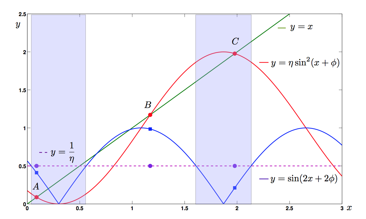
Figure D.1: Illustration of the statement of Corollary D.7. The parameter vector $\boldsymbol{\theta}$ in (D.39) is set to $(2,-0.3)$. Non-trivial equilibria $x_{0}=0.088$ (point $A$), $x_{0}=1.172$ (point $B$), $x_{0}=1.977$ (point $C$) are provided by the relation (D.41). Grey bands represent the regions where the sufficient stability conditions (D.40) in the statement of the corollary are satisfied; the equilibria that correspond to the points $A$ and $C$ are hence stable.

D.3 Fixed points of the reservoir map and their stability

In this section we consider the discrete time TDR, we characterize its fixed points and establish sufficient conditions for their stability which, as we will show, are analogous to the ones that we obtained for the continuous time case.

We place ourselves in the autonomous regime, that is, $I(t)=0$ in the time-delay differential equation (B.1) and $\mathbf{I}(t)={\bf 0}_{N}$ in the associated recursion (B.3). In this case, we can state the following proposition that shows that there is a bijective correspondence between the equilibria of the discrete and continuous time TDRs.

Proposition D.9

The point $x_{0}\in\mathbb{R}$ is an equilibrium of the time-delay differential equation (D.21) in autonomous regime, that is when $I(t)=0$, if and only if the vector $\mathbf{x}_{0}:=x_{0}\mathbf{i}_{N}$ is a fixed point of the $N$-dimensional discretized nonlinear time-delay reservoir

$$\dot{\mathbf{x}}(t)=F(\mathbf{x}(t-1),\mathbf{I}(t),\boldsymbol{\theta})$$ (D.43)

in autonomous regime, that is, when $\mathbf{I}(t)={\bf 0}_{N}$.

Proof. Suppose first that $x_{0}$ is an equilibrium of the time-delay differential equation (D.21) and hence satisfies $x_{0}=f(x_{0},0,\boldsymbol{\theta})$. In order to show that $F(\mathbf{x}(t-1),\mathbf{0}_{N},\boldsymbol{\theta})=\mathbf{x}_{0}$, we evaluate the components of the right hand side of (B.2) at $\mathbf{x}_{0}$ and obtain

$$(F(\mathbf{x}_{0},{\bf 0}_{N},\boldsymbol{\theta}))_{i}={e}^{-i\xi}x_{0}+(1-{e}^{-\xi})\sum^{i-1}_{j=0}{e}^{-j\xi}f(x_{0},0,\boldsymbol{\theta})={e}^{-i\xi}x_{0}+(1-{e}^{-\xi})\sum^{i-1}_{j=0}{e}^{-j\xi}x_{0}=x_{0},$$

as required. The proof of the converse implication is also straightforward using (B.2). $\square$

We now provide sufficient conditions for the stability of the fixed points of the type $\mathbf{x}_{0}=x_{0}\mathbf{i}_{N}$ described in Proposition D.9. The asymptotic stability (respectively, stability) of those fixed points is guaranteed whenever the connectivity matrix $A(\mathbf{x}_{0},\boldsymbol{\theta})$ in (B.9) satisfies $\rho(A(\mathbf{x}_{0},\boldsymbol{\theta}))<1$ (respectively, $\rho(A(\mathbf{x}_{0},\boldsymbol{\theta}))\leq 1)$). Since it is not possible to compute the eigenvalues of $A(\mathbf{x}_{0},\boldsymbol{\theta})$ for an arbitrary number of neurons $N$, we proceed by finding upper bounds of its spectral radius $\rho(A(\mathbf{x}_{0},\boldsymbol{\theta}))$. This can be done with the help of the Gershgorin disks theorem (see for instance Corollary 6.1.5 in [Horn 13]) or by using a matrix norm $|||\cdot|||$ and noting that $\rho(A(\mathbf{x}_{0},\boldsymbol{\theta}))\leq|||A(\mathbf{x}_{0},\boldsymbol{\theta})|||$. After a detailed study using all these possibilities we found that the best result is obtained by using the maximum row sum matrix norm $|||A(\mathbf{x}_{0},\boldsymbol{\theta})|||_{\infty}$ defined in Section A, which allows us to formulate the following result.

Theorem D.10

Let $\mathbf{x}_{0}=x_{0}\mathbf{i}_{N}$ be a fixed point of the $N$-dimensional recursion $\mathbf{x}(t)=F(\mathbf{x}(t-1),\mathbf{I}(t),\boldsymbol{\theta})$ in autonomous regime. Then, $\mathbf{x}_{0}\in\mathbb{R}^{N}$ is asymptotically stable (respectively stable) if $|\partial_{{x}}f({x}_{0},{0},\boldsymbol{\theta})|<1$ (respectively, $|\partial_{{x}}f({x}_{0},{0},\boldsymbol{\theta})|\leq 1$).

Proof. We first recall that the connectivity matrix (B.9) of the discretized nonlinear TDR with $N$ virtual nodes is given by

$$A(\mathbf{x}_{0},\boldsymbol{\theta}):={\small\left(\begin{array}[]{cccccc}\Phi&0&\ldots&0&{e^{-\xi}}\\ \Phi{e^{-\xi}}&\Phi&\ldots&0&{e^{-2\xi}}\\ \Phi e^{-2\xi}&\Phi e^{-\xi}&\ldots&0&{e^{-3\xi}}\\ \vdots&\vdots&\vdots&&\vdots\\ \Phi e^{-(N-1)\xi}&\Phi e^{-(N-2)\xi}&\ldots&\Phi e^{-\xi}&\Phi+{e^{-N\xi}}\end{array}\right)},$$ (D.49)

where $\Phi:=(1-e^{-\xi})\cdot\partial_{{x}}f({x}_{0},{0},\boldsymbol{\theta})$ and recall that $\partial_{{x}}f({x}_{0},{0},\boldsymbol{\theta})$ is the first derivative of the nonlinear kernel $f$ in (B.1) with respect to the first argument and computed at the point $({\bf x}_{0},{\bf 0}_{N},\boldsymbol{\theta})$, with $\xi=\log(1+d)$ and $d\in(0,1]$ the Euler discretization step or, equivalently, the separation between the virtual neurons. We will use the notation $f^{\prime}_{x_{0}}:=\partial_{{x}}f({x}_{0},{0},\boldsymbol{\theta})$ in what follows.

We proceed by finding sufficient conditions on $f^{\prime}_{x_{0}}$ that guarantee that the spectral radius of $A(\mathbf{x}_{0},\boldsymbol{\theta})$ is bounded above by $1$. These conditions will be obtained by enforcing $|||A(\mathbf{x}_{0},\boldsymbol{\theta})|||_{\infty}<1$ and by recalling that

$$\rho(A(\mathbf{x}_{0},\boldsymbol{\theta}))\leq|||A(\mathbf{x}_{0},\boldsymbol{\theta})|||_{\infty}=\max_{1\leq i\leq N}\sum^{N}_{j=1}|a_{ij}|.$$ (D.50)

In the view of the rows of the matrix $A(\mathbf{x}_{0},\boldsymbol{\theta})$, it is clear that $|||A(\mathbf{x}_{0},\boldsymbol{\theta})|||_{\infty}$ is given by the sum of the absolute values of one of the rows with numbers $1$, $N-1$, or $N$. We can hence write

$$|||A(\mathbf{x}_{0},\boldsymbol{\theta})|||_{\infty}={\max}\Bigg{\{}\begin{array}[]{cl}u:=&e^{-\xi}+(1-e^{-\xi})|f^{\prime}_{x_{0}}|\\ v:=&e^{-(N-1)\xi}+(1-e^{-(N-1)\xi})|f^{\prime}_{x_{0}}|\\ w:=&|e^{-N\xi}+(1-e^{-\xi})f^{\prime}_{x_{0}}|+e^{-\xi}(1-e^{-(N-1)\xi})|f^{\prime}_{x_{0}}|\end{array}\Bigg{\}}.$$ (D.51)

It can be easily verified that this expression can be split into two cases, namely

$$|||A(\mathbf{x}_{0},\boldsymbol{\theta})|||_{\infty}= \max\{u,w\}, |f^{\prime}_{x_{0}}|\leq 1$$ if (D.52a)

$$|||A(\mathbf{x}_{0},\boldsymbol{\theta})|||_{\infty}= \max\{v,w\}, |f^{\prime}_{x_{0}}|\geq 1$$ if (D.52b)

Additionally, by definition of the absolute value, we have two cases:

$$|f^{\prime}_{x_{0}}|= f^{\prime}_{x_{0}}, f^{\prime}_{x_{0}}\in[0,+\infty)$$ if (D.53a)

$$|f^{\prime}_{x_{0}}|= -f^{\prime}_{x_{0}}, f^{\prime}_{x_{0}}\in(-\infty,0)$$ if (D.53b)

and hence

$$|e^{-N\xi}+(1-e^{-\xi})f^{\prime}_{x_{0}}|= e^{-N\xi}+(1-e^{-\xi})f^{\prime}_{x_{0}}, f^{\prime}_{x_{0}}\in\bigg{[}-\dfrac{e^{-N\xi}}{1-e^{-\xi}},+\infty\bigg{)}$$ if (D.54a)

$$|e^{-N\xi}+(1-e^{-\xi})f^{\prime}_{x_{0}}|= -e^{-N\xi}-(1-e^{-\xi})f^{\prime}_{x_{0}}, f^{\prime}_{x_{0}}\in\bigg{(}-\infty,-\dfrac{e^{-N\xi}}{1-e^{-\xi}}\bigg{)}$$ if . (D.54b)

We now consider in detail all the possible combinations of cases that provide the conditions on $f^{\prime}_{x_{0}}$ that ensure stability by enforcing that $|||A(\mathbf{x}_{0},\boldsymbol{\theta})|||_{\infty}<1$.

Case I (D.52a), (D.53a), (D.54a).

On one hand, (D.52a), (D.53a), (D.54a) give that $f^{\prime}_{x_{0}}\in[0,1)$. On the other hand (D.52a) amounts to

$$|||A(\mathbf{x}_{0},\boldsymbol{\theta})|||_{\infty}=\max\{u,w\}= u, f^{\prime}_{x_{0}}\in(-\infty,1]$$ if (D.55a)

$$|||A(\mathbf{x}_{0},\boldsymbol{\theta})|||_{\infty}=\max\{u,w\}= w, f^{\prime}_{x_{0}}\in(1,+\infty).$$ if (D.55b)

Notice that since $f^{\prime}_{x_{0}}\in[0,1)$, then these cases reduce to:

$$|||A(\mathbf{x}_{0},\boldsymbol{\theta})|||_{\infty}=u,$$ (D.56)

and hence

$$\rho(A(\mathbf{x}_{0},\boldsymbol{\theta}))\leq u=e^{-\xi}+(1-e^{-\xi})f^{\prime}_{x_{0}}<1\enspace\Longrightarrow f^{\prime}_{x_{0}}\in(-\infty,1).$$

We finally write that in this case stability is guaranteed whenever

$$f^{\prime}_{x_{0}}\in I1:=[0,1).$$ (D.57)

Case II (D.52a), (D.53a), (D.54b).

On one hand, (D.52a), (D.53a) imply that $f^{\prime}_{x_{0}}\in[0,1)$ but by (D.54b) it is required at the same time that $f^{\prime}_{x_{0}}\in(-\infty,-\dfrac{e^{-N\xi}}{1-e^{-\xi}})$ which immediately yields in this case:

$$f^{\prime}_{x_{0}}\in I2:=\emptyset.$$ (D.58)

Case III (D.52a), (D.53b), (D.54a).

On one hand, (D.52a), (D.53b), (D.54a) imply that

$$f^{\prime}_{x_{0}}\in\Big{[}\max\Big{\{}-1,-\dfrac{e^{-N\xi}}{1-e^{-\xi}}\Big{\}},0\Big{)}.$$ (D.59)

On the other hand, the condition that defines (D.52a) amounts to

$$\!\!\!\!\!\!\!\!\!\!\!\!\!\!\!\!\!\!\!\!\!\!\!\!\!\!\!\!|||A(\mathbf{x}_{0},\boldsymbol{\theta})|||_{\infty}=\max\{u,w\}= u, f^{\prime}_{x_{0}}\in\bigg{[}-\dfrac{e^{-\xi}-e^{-N\xi}}{|2-3e^{-\xi}+e^{-N\xi}|},\dfrac{e^{-\xi}-e^{-N\xi}}{|2-3e^{-\xi}+e^{-N\xi}|}\bigg{]}$$ if (D.60a)

$$\!\!\!\!\!\!\!\!\!\!\!\!\!\!\!\!\!\!\!\!\!\!\!\!\!\!\!\!|||A(\mathbf{x}_{0},\boldsymbol{\theta})|||_{\infty}=\max\{u,w\}= w, \begin{array}[]{l}{\rm if}\enspace f^{\prime}_{x_{0}}\in\bigg{(}-\infty,-\dfrac{e^{-\xi}-e^{-N\xi}}{|2-3e^{-\xi}+e^{-N\xi}|}\bigg{)}\\ \cup\bigg{(}\dfrac{e^{-\xi}-e^{-N\xi}}{|2-3e^{-\xi}+e^{-N\xi}|},+\infty\bigg{)}\end{array}.$$ (D.60d)

Notice now that at the same time we require that $|||A(\mathbf{x}_{0},\boldsymbol{\theta})|||_{\infty}<1$. Hence for the case (D.60a) we have

$$\rho(A(\mathbf{x}_{0},\boldsymbol{\theta}))\leq|||A(\mathbf{x}_{0},\boldsymbol{\theta})|||_{\infty}=u=e^{-\xi}-(1-e^{-\xi})f^{\prime}_{x_{0}}<1\Longrightarrow f^{\prime}_{x_{0}}\in(-1,+\infty)$$ (D.61)

which put together with the conditions for $f^{\prime}_{x_{0}}$ in (D.60a), (D.61), and (D.59) yields

$$f^{\prime}_{x_{0}}\in I3:=\Bigg{(}\max\Bigg{\{}-1,-\dfrac{e^{-N\xi}}{1-e^{-\xi}},-\dfrac{e^{-\xi}-e^{-N\xi}}{|2-3e^{-\xi}+e^{-N\xi}|}\Bigg{\}},0\Bigg{)}.$$ (D.62)

We now consider the case (D.60d) and in an analogous way using (D.50) we have that

$$\rho(A(\mathbf{x}_{0},\boldsymbol{\theta}))\leq|||A(\mathbf{x}_{0},\boldsymbol{\theta})|||_{\infty}= w=e^{-N\xi}+(1-2e^{-\xi}+e^{-N\xi})f^{\prime}_{x_{0}}<1\Longrightarrow$$

$$f^{\prime}_{x_{0}}\in\bigg{(}-\dfrac{1-e^{-N\xi}}{|1-2e^{-\xi}+e^{-N\xi}|},\dfrac{1-e^{-N\xi}}{|1-2e^{-\xi}+e^{-N\xi}|}\bigg{)}$$ (D.63)

If we put together the conditions for $f^{\prime}_{x_{0}}$ in (D.60d), (D.3), and (D.59) we obtain

$$f^{\prime}_{x_{0}}\in I4:=\Bigg{(}\max\Bigg{\{}-1,-\dfrac{e^{-N\xi}}{1-e^{-\xi}},-\dfrac{1-e^{-N\xi}}{|1-2e^{-\xi}+e^{-N\xi}|}\Bigg{\}},-\dfrac{e^{-\xi}-e^{-N\xi}}{|2-3e^{-\xi}+e^{-N\xi}|}\Bigg{)}.$$ (D.64)

Case IV (D.52a), (D.53b), (D.54b).

On one hand, (D.52a), (D.53b), (D.54b) imply that

$$f^{\prime}_{x_{0}}\in\Big{(}-1,-\dfrac{e^{-N\xi}}{1-e^{-\xi}}\Big{)}.$$ (D.65)

On the other hand, the case (D.52a) amounts to

$$|||A(\mathbf{x}_{0},\boldsymbol{\theta})|||_{\infty}=\max\{u,w\}= u, f^{\prime}_{x_{0}}\in\bigg{[}-\dfrac{1+e^{-(N-1)\xi}}{1-e^{-(N-1)\xi}},+\infty\bigg{)}$$ if (D.66a)

$$|||A(\mathbf{x}_{0},\boldsymbol{\theta})|||_{\infty}=\max\{u,w\}= w, f^{\prime}_{x_{0}}\in\bigg{(}-\infty,-\dfrac{1+e^{-(N-1)\xi}}{1-e^{-(N-1)\xi}}\bigg{)}$$ if . (D.66b)

It can be easily verified that the condition defining (D.66b) is incompatible with (D.65) since the relation $-1\geq-\dfrac{1+e^{-(N-1)\xi}}{1-e^{-(N-1)\xi}}$ holds for any $\xi\in(0,1]$ and $N\in\mathbb{N}$. We hence conclude using the case (D.66a) that

$$\rho(A(\mathbf{x}_{0},\boldsymbol{\theta}))\leq|||A(\mathbf{x}_{0},\boldsymbol{\theta})|||_{\infty}=u=e^{-\xi}-(1-e^{-\xi})f^{\prime}_{x_{0}}<1\Longrightarrow f^{\prime}_{x_{0}}\in(-1,+\infty).$$

Hence, together with (D.65) this amounts to

$$f^{\prime}_{x_{0}}\in I5:=\Big{(}-1,-\dfrac{e^{-N\xi}}{1-e^{-\xi}}\Big{)}.$$ (D.67)

Case V (D.52b), (D.53a), (D.54a).

On one hand, (D.52b), (D.53a), (D.54a) imply that

$$f^{\prime}_{x_{0}}\in[1,+\infty].$$ (D.68)

On the other hand, the case (D.52a) amounts to

$$|||A(\mathbf{x}_{0},\boldsymbol{\theta})|||_{\infty}=\max\{v,w\}= v, f^{\prime}_{x_{0}}\in(-\infty,-1]$$ if (D.69a)

$$|||A(\mathbf{x}_{0},\boldsymbol{\theta})|||_{\infty}=\max\{v,w\}= w, f^{\prime}_{x_{0}}\in(-1,+\infty)$$ if . (D.69b)

Due to (D.68)

$$\rho(A(\mathbf{x}_{0},\boldsymbol{\theta}))\leq|||A(\mathbf{x}_{0},\boldsymbol{\theta})|||_{\infty}=w=e^{-N\xi}+(1-e^{-N\xi})f^{\prime}_{x_{0}}<1\Longrightarrow f^{\prime}_{x_{0}}\in(-\infty,1),$$

which yields

$$f^{\prime}_{x_{0}}\in I6:=\emptyset.$$ (D.70)

Case VI (D.52b), (D.53a), (D.54b).

The conditions (D.52b), (D.53a), and (D.54b) immediately yield

$$f^{\prime}_{x_{0}}\in I7:=\emptyset.$$ (D.71)

Case VII (D.52b), (D.53b), (D.54a).

On one hand, (D.52b), (D.53b), (D.54a) imply that

$$f^{\prime}_{x_{0}}\in\Big{[}-\dfrac{e^{-N\xi}}{1-e^{-\xi}},-1\Big{]}.$$ (D.72)

On the other hand, the case (D.52b) amounts to

$$|||A(\mathbf{x}_{0},\boldsymbol{\theta})|||_{\infty}=\max\{v,w\}= v, f^{\prime}_{x_{0}}\in\bigg{(}-\infty,-\dfrac{e^{-(N-1)\xi}}{2-e^{-(N-1)\xi}}\bigg{]}$$ if , (D.73a)

$$|||A(\mathbf{x}_{0},\boldsymbol{\theta})|||_{\infty}=\max\{v,w\}= w, f^{\prime}_{x_{0}}\in\bigg{(}-\dfrac{e^{-(N-1)\xi}}{2-e^{-(N-1)\xi}},+\infty\bigg{)}.$$ if (D.73b)

Hence, for the case (D.73a) we have

$$\rho(A(\mathbf{x}_{0},\boldsymbol{\theta}))\leq|||A(\mathbf{x}_{0},\boldsymbol{\theta})|||_{\infty}=v=e^{-(N-1)\xi}-(1-e^{-(N-1)\xi})f^{\prime}_{x_{0}}<1\Longrightarrow f^{\prime}_{x_{0}}\in(-1,+\infty)$$

which due to (D.72) gives

$$f^{\prime}_{x_{0}}\in I8:=\emptyset.$$ (D.74)

We now consider the case (D.73b) and in an analogous way we have that

$$\rho(A(\mathbf{x}_{0},\boldsymbol{\theta}))\leq|||A(\mathbf{x}_{0},\boldsymbol{\theta})|||_{\infty}= w=e^{-N\xi}+(1-2e^{-\xi}+e^{-N\xi})f^{\prime}_{x_{0}}<1\Longrightarrow$$

$$f^{\prime}_{x_{0}}\in\bigg{(}-\dfrac{1-e^{-N\xi}}{|1-2e^{-\xi}+e^{-N\xi}|},\dfrac{1-e^{-N\xi}}{|1-2e^{-\xi}+e^{-N\xi}|}\bigg{)}.$$ (D.75)

Hence by (D.3), (D.73b) and (D.72) we can write

$$f^{\prime}_{x_{0}}\in I9:=\bigg{(}\max\bigg{\{}-\dfrac{e^{-N\xi}}{1-e^{-\xi}},-\dfrac{e^{-(N-1)\xi}}{2-e^{-(N-1)\xi}},-\dfrac{1-e^{-N\xi}}{|1-2e^{-\xi}+e^{-N\xi}|}\bigg{\}},-1\bigg{]}=\emptyset,$$ (D.76)

where the last equality follows from the fact that $-\dfrac{e^{-(N-1)\xi}}{2-e^{-(N-1)\xi}}\geq-1$, for any $\xi\in(0,1]$ and $N\in\mathbb{N}$.

Case VIII (D.52b), (D.53b), (D.54b).

On one hand, (D.52b), (D.53b), (D.54b) imply that

$$f^{\prime}_{x_{0}}\in\Big{(}-\infty,\min\bigg{\{}-\dfrac{e^{-N\xi}}{1-e^{-\xi}},-1\bigg{\}}\Big{)}.$$ (D.77)

On the other hand, the case (D.52b) amounts to

$$|||A|||_{\infty}=\max\{v,w\}= v, f^{\prime}_{x_{0}}\in\bigg{[}-\dfrac{1+e^{-\xi}}{1-e^{-\xi}},+\infty\bigg{)}$$ if (D.78a)

$$|||A|||_{\infty}=\max\{v,w\}= w, f^{\prime}_{x_{0}}\in\bigg{(}-\infty,-\dfrac{1+e^{-\xi}}{1-e^{-\xi}}\bigg{)}.$$ if (D.78b)

Hence for the case (D.78a) we have

$$\rho(A(\mathbf{x}_{0},\boldsymbol{\theta}))\leq|||A(\mathbf{x}_{0},\boldsymbol{\theta})|||_{\infty}=v=e^{-(N-1)\xi}-(1-e^{-(N-1)\xi})f^{\prime}_{x_{0}}<1\Longrightarrow f^{\prime}_{x_{0}}\in(-1,+\infty)$$

which due to (D.77) implies that

$$f^{\prime}_{x_{0}}\in I10:=\emptyset.$$ (D.79)

We now consider the case (D.78b) and in an analogous way we have that

$$\rho(A(\mathbf{x}_{0},\boldsymbol{\theta}))\leq|||A(\mathbf{x}_{0},\boldsymbol{\theta})|||_{\infty}=w=-e^{-N\xi}+(-1+e^{-N\xi})f^{\prime}_{x_{0}}<1\Longrightarrow f^{\prime}_{x_{0}}\in\bigg{(}-\dfrac{1+e^{-N\xi}}{1-e^{-N\xi}},+\infty\bigg{)}.$$ (D.80)

Hence by (D.80), (D.78b) and (D.77) we can write

$$f^{\prime}_{x_{0}}\in I11:=\bigg{(}-\dfrac{1+e^{-N\xi}}{1-e^{-N\xi}},\min\bigg{\{}-\dfrac{e^{-N\xi}}{1-e^{-\xi}},-1,-\dfrac{1+e^{-\xi}}{1-e^{-\xi}}\bigg{\}}\bigg{)}=\emptyset,$$ (D.81)

for any $\xi\in(0,1]$ and $N\in\mathbb{N}$.

Finally, we put together all the non-empty intervals provided by the Cases I-VIII that guarantee that when $f^{\prime}_{x_{0}}$ belongs to them, then the fixed point $\mathbf{x}_{0}$ is stable:

$$f^{\prime}_{x_{0}}\in\Big{(}-1,-\dfrac{e^{-N\xi}}{1-e^{-\xi}}\Big{)} \cup\Bigg{(}\max\Bigg{\{}-1,-\dfrac{e^{-N\xi}}{1-e^{-\xi}},-\dfrac{1-e^{-N\xi}}{|1-2e^{-\xi}+e^{-N\xi}|}\Bigg{\}},-\dfrac{e^{-\xi}-e^{-N\xi}}{|2-3e^{-\xi}+e^{-N\xi}|}\Bigg{)}$$

$$\cup\Bigg{(}\max\Bigg{\{}-1,-\dfrac{e^{-N\xi}}{1-e^{-\xi}},-\dfrac{e^{-\xi}-e^{-N\xi}}{|2-3e^{-\xi}+e^{-N\xi}|}\Bigg{\}},0\Bigg{)}\cup[0,1).$$ (D.82)

Now, it is easy to see that

$$\max\Bigg{\{}-1,-\dfrac{e^{-N\xi}}{1-e^{-\xi}},-\dfrac{e^{-\xi}-e^{-N\xi}}{|2-3e^{-\xi}+e^{-N\xi}|}\Bigg{\}}\geq-1,$$

$$\max\Bigg{\{}-1,-\dfrac{e^{-N\xi}}{1-e^{-\xi}},-\dfrac{1-e^{-N\xi}}{|1-2e^{-\xi}+e^{-N\xi}|}\Bigg{\}}\geq-1,$$

and hence the condition (D.3) reduces to

$$|f^{\prime}_{x_{0}}|<1.$$

Notice that the proof remains valid for the case of (not necessary asymptotic) stability in the statement of the theorem. In this case we require

$$\rho(A(\mathbf{x}_{0},\boldsymbol{\theta}))\leq|||A(\mathbf{x}_{0},\boldsymbol{\theta})|||_{\infty}=\max_{1\leq i\leq N}\sum^{N}_{j=1}|a_{ij}|\leq 1,$$

which results in the condition

$$|f^{\prime}_{x_{0}}|\leq 1,$$

as required. $\square$

The following theorem provides the characteristic polynomial of the connectivity matrix $A(\mathbf{x}_{0},\boldsymbol{\theta})$ and an explicit expression for its spectral radius under some conditions. Another way to find upper bounds for this spectral radius would consist of using the Cauchy bound [Rahm 02] of this polynomial. In our experience this approach produces mediocre results in comparison with the statement in Theorem D.10.

Theorem D.11

Let $A(\mathbf{x}_{0},\boldsymbol{\theta})$ be the connectivity matrix of the reservoir map in (B.9). Define $\Phi:=(1-e^{-\xi})f^{\prime}_{x_{0}}$ and let $\left\{\lambda_{1},\dots,\lambda_{N}\right\}$ be the roots of the polynomial equation

$$\lambda^{N}-\left(\dfrac{e^{-N\xi}}{\Phi}+N\right)\lambda^{N-1}+\sum^{N-2}_{j=0}\left(\begin{array}[]{c}N\\ j\end{array}\right)(-1)^{N-j}\lambda^{j}=0.$$ (D.83)

Then $\rho(A(\mathbf{x}_{0},\boldsymbol{\theta}))=\max\left\{|\Phi\lambda_{1}|,\dots,|\Phi\lambda_{N}|\right\}$. Moreover, if (D.83) has a root $\lambda$ such that $\lambda>1$, then $\rho(A(\mathbf{x}_{0},\boldsymbol{\theta}))=\lambda|\Phi|$ necessarily.

Proof. Define first $B:=\dfrac{1}{\Phi}A(\mathbf{x}_{0},\boldsymbol{\theta})$. We then write

$$B:={\small\left(\begin{array}[]{cccccc}1&0&\ldots&0&\dfrac{e^{-\xi}}{\Phi}\\ {e^{-\xi}}&1&\ldots&0&\dfrac{e^{-2\xi}}{\Phi}\\ e^{-2\xi}&e^{-\xi}&\ldots&0&\dfrac{e^{-3\xi}}{\Phi}\\ \vdots&\vdots&\vdots&&\vdots\\ e^{-(N-1)\xi}&e^{-(N-2)\xi}&\ldots&e^{-\xi}&1+\dfrac{e^{-N\xi}}{\Phi}\end{array}\right)}.$$

Let $\mathbf{v}=(v_{1},\dots,v_{N})$ be an eigenvector of $B$ with eigenvalue $\lambda$, that is, $B\mathbf{v}=\lambda\mathbf{v}$. This equality can be rewritten as

$$\left\{\begin{array}[]{lcl}v_{1}&=&\dfrac{e^{-\xi}}{(\lambda-1)\Phi}v_{N},\\ v_{2}&=&\dfrac{e^{-2\xi}}{(\lambda-1)\Phi}v_{N}\dfrac{\lambda}{\lambda-1},\\ v_{3}&=&\dfrac{e^{-3\xi}}{(\lambda-1)\Phi}v_{N}\dfrac{\lambda^{2}}{(\lambda-1)^{2}},\\ \vdots&\vdots&\ \ \ \ \ \ \ \ \ \vdots\\ v_{N-1}&=&\dfrac{e^{-(N-1)\xi}}{(\lambda-1)\Phi}v_{N}\dfrac{\lambda^{N-2}}{(\lambda-1)^{N-2}},\end{array}\right.$$ (D.84)

together with the identity

$$\sum^{N}_{j=1}b_{Nj}v_{j}=\lambda v_{N},$$

which is equivalent to

$$\dfrac{v_{N}}{(\lambda-1)\Phi}e^{-N\xi}\left(1+\dfrac{\lambda}{\lambda-1}+\dfrac{\lambda^{2}}{(\lambda-1)^{2}}+\cdots+\dfrac{\lambda^{N-2}}{(\lambda-1)^{N-2}}\right)+v_{N}\left(1+\dfrac{e^{-N\xi}}{\Phi}\right)=\lambda v_{N},$$

or, equivalently, to

$$v_{N}\left(\dfrac{e^{-N\xi}}{\Phi}\dfrac{\lambda^{N-1}-(\lambda-1)^{N-1}}{(\lambda-1)^{N-1}}+(\lambda-1)+\dfrac{e^{-N\xi}}{\Phi}\right)=0.$$

If we assume that $b_{N}\neq 0$ and $\lambda\neq 1$, this amounts to

$$\dfrac{(\lambda-1)^{N}}{\lambda^{N-1}}=\dfrac{e^{-N\xi}}{\Phi}.$$

Consequently, the eigenvalues of $A$ are given by the roots $\left\{\lambda_{1},\dots,\lambda_{N}\right\}$ of the polynomial equation

$$\lambda^{N}-\left(\dfrac{e^{-N\xi}}{\Phi}+N\right)\lambda^{N-1}+\sum^{N-2}_{j=0}\left(\begin{array}[]{c}N\\ j\end{array}\right)(-1)^{N-j}\lambda^{j}=0$$

and hence

$$\rho(A(\mathbf{x}_{0},\boldsymbol{\theta}))=\max\left\{|\Phi\lambda_{1}|,\dots,|\Phi\lambda_{N}|\right\}.$$

If there exists some $\lambda>1$, the expressions (D.84) show that the eigenvector $\mathbf{v}$ of $B$ (or of $-B$ if $\Phi<0$) can be chosen positive. In that situation Corollary 8.1.30 in [Horn 13] guarantees that $\rho(B)=\lambda$ with $\lambda>1$ the eigenvalue corresponding to $\mathbf{v}$ and hence $\rho(A(\mathbf{x}_{0},\boldsymbol{\theta}))=|\Phi\lambda|$ as required. $\square$

Appendix E Robustness of the empirical tests with respect to the choice of nonlinear kernel

In this section we show the robustness of the empirical results in Sections 1.1 and 2 of the paper with respect to the choice of the nonlinear kernel used in the construction of the TDR.

First, in Section 1.1 we carried out an experiment using the Ikeda kernel and a quadratic memory task that showed that optimal performance is obtained when the input mean and variance are tuned so that the dynamics of the reservoir takes place in the neighborhood of a stable steady state and making sure that multimodality is avoided. We have repeated here the same experiment but, this time, using the Mackey-Glass kernel. More specifically, we nonsider a TDR with $N=20$ neurons $d=0.943$, $\gamma=4.7901$, $\eta=1.3541$, and $p=2$. As we explained in Corollary D.6, with these parameter values $x_{0}=-\sqrt{\eta-1}=-0.5951$ is an equilibrium that satisfies the sufficient conditions for asymptotic stability. In order to verify that the optimal performance is obtained when the RC operates in a neighborhood of that stable equilibrium, we study the normalized mean square error (NMSE) exhibited by a TDR initialized at $x_{0}=-0.5951$ when we present to it a quadratic memory task. More specifically, we inject in a TDR under study an independent and identically normally distributed signal $z(t)$ with mean zero and variance $10^{-4}$ and we then train a linear readout $W_{{\rm out}}$ (obtained with a ridge penalization of $\lambda=10^{-15}$) in order to recover the quadratic function $z(t-1)^{2}+z(t-2)^{2}+z(t-3)^{2}$ out of the reservoir output. The top left panel in Figure E.1 shows how the NMSE behaves as a function of the mean and the variance of the input mask ${\bf c}$. It is clear that by modifying any of these two parameters we control how far the reservoir dynamics separates from the stable equilibrium, which we quantitatively evaluate in the two bottom panels by representing the RC performance in terms of the mean and the variance of the resulting reservoir output. Both panels depict how the injection of a signal slightly shifted in mean or with a sufficiently high variance results in reservoir outputs that separate from the stable equilibrium and in a severely degraded performance. An important factor in this deterioration seems to be the multi modality, that is, if the shifting in mean or the input signal variance are large enough then the reservoir output visits the stability basin of the other stable point placed at $x_{0}=\sqrt{\eta-1}=0.5951$; in the top right and bottom panels we have marked with red color the values for which bimodality has occurred so that the negative effect of this phenomenon is noticeable.

Figure E.1: Behavior of the performance of a Mackey-Glass based reservoir in a quadratic memory task as a function of the mean and the variance of the input mask. The modification of any of these two parameters influences how the reservoir dynamics separates from the stable equilibrium. The top panels show how the performance degrades very quickly as soon as the mean and the variance of the input mask (and hence of the input signal) separate from zero. The bottom panels depict the reservoir performance as a function of the various output means and variances obtained when changing the input means and variances. In the top right and bottom panels we have indicated with red markers the cases in which the reservoir visits the stability basin of a contiguous equilibrium hence showing how unimodality is associated to optimal performance.

Second, in Section 2 we used a Mackey-Glass based reservoir to compare the empirical performance surfaces in terms of various parameters with that coming from the formula (13) that was obtained as a result of modeling the reservoir with an approximating VAR(1) process. In this section we have repeated the same exercise with an Ikeda based reservoir in order to show that the formula (13) produces in this case results of comparable quality. The outcome of this experiment are contained in Figure E.2 where we represent the normalized mean square error as a function of the distance between neurons and the feedback gain $\eta$. The other fixed parameter values used are $\gamma=0.523$ and $\phi=0.3106$; the reservoir was constructed using 20 neurons and we presented to it the three-lag quadratic memory task corresponding to the diagonal matrix $Q$ with diagonal entries given by the vector $(0,1,1,1)$. The optimal output mask ${\mathbf{W}}_{{\rm out}}$ was computed using a ridge regression with $\lambda=10^{-15}$. As it can be seen in the figure, we restrict the values of the parameter $\eta$ to the interval $[0,1]$ which ensures, using one of the results in Corollary D.7, that the TDR exhibits for each value of $\eta$ a unique equilibrium (unimodality is hence guaranteed) that is always stable. The TDR is always initialized at that stable configuration.

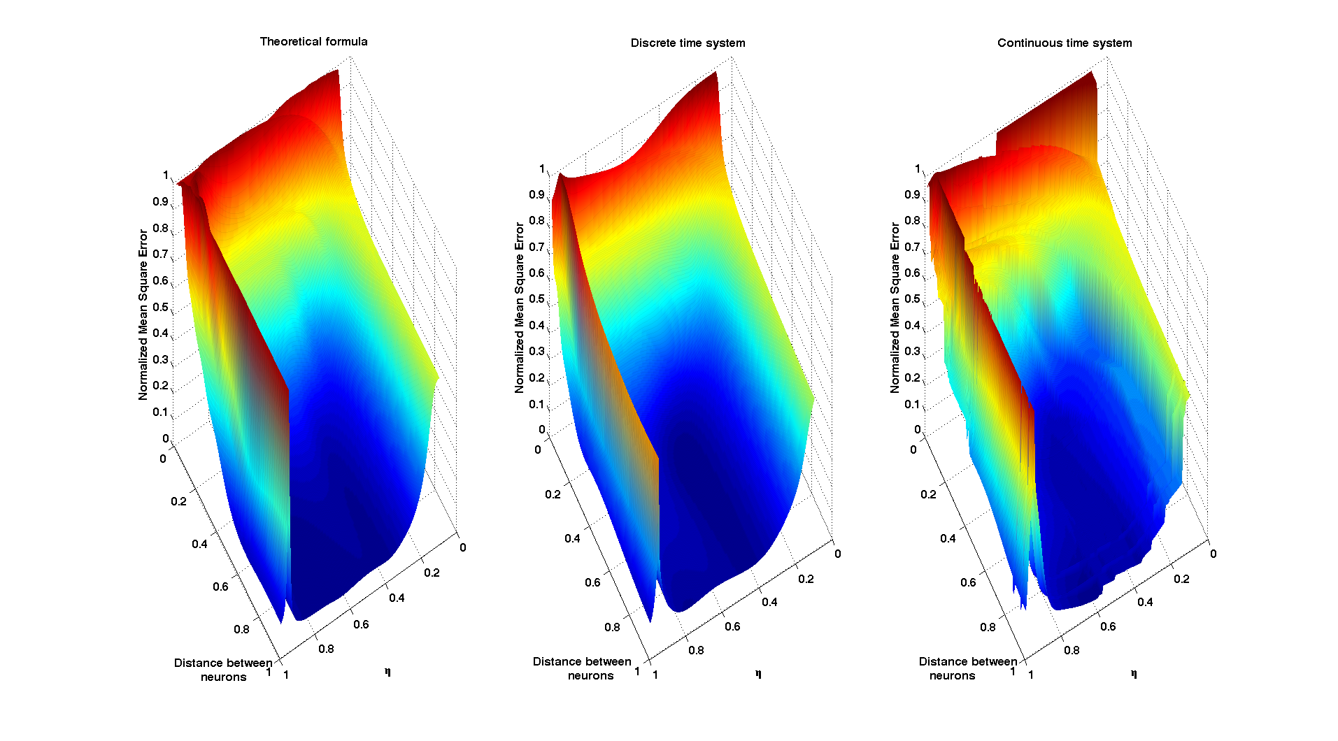
Figure E.2: Error surfaces exhibited by an Ikeda based reservoir computer in a 3-lag quadratic memory task, as a function of the distance between neurons and the parameter $\eta$. The points in the surfaces of the middle and right panels are the result of Monte Carlo evaluations of the NMSE exhibited by the discrete and continuous time TDRs, respectively. The left panel was constructed using the formula (13) that is obtained as a result of modeling the reservoir with an approximating VAR(1) process.

References

- [Appe 11] L. Appeltant, M. C. Soriano, G. Van der Sande, J. Danckaert, S. Massar, J. Dambre, B. Schrauwen, C. R. Mirasso, and I. Fischer. “Information processing using a single dynamical node as complex system”. Nature Communications, Vol. 2, p. 468, Jan. 2011.
- [Atiy 00] A. F. Atiya and A. G. Parlos. “New results on recurrent network training: unifying the algorithms and accelerating convergence”. IEEE transactions on neural networks / a publication of the IEEE Neural Networks Council, Vol. 11, No. 3, pp. 697–709, Jan. 2000.
- [Boyd 85] S. Boyd and L. Chua. “Fading memory and the problem of approximating nonlinear operators with Volterra series”. IEEE Transactions on Circuits and Systems, Vol. 32, No. 11, pp. 1150–1161, Nov. 1985.
- [Brun 13] D. Brunner, M. C. Soriano, C. R. Mirasso, and I. Fischer. “Parallel photonic information processing at gigabyte per second data rates using transient states”. Nature Communications, Vol. 4, No. 1364, 2013.
- [Caul 10] H. J. Caulfield and S. Dolev. “Why future supercomputing requires optics”. Nature Photonics, Vol. 4, No. 5, pp. 261–263, May 2010.
- [Croo 07] N. Crook. “Nonlinear transient computation”. Neurocomputing, Vol. 70, pp. 1167–1176, 2007.
- [Crut 10] J. P. Crutchfield, W. L. Ditto, and S. Sinha. “Introduction to focus issue: intrinsic and designed computation: information processing in dynamical systems-beyond the digital hegemony”. Chaos (Woodbury, N.Y.), Vol. 20, No. 3, p. 037101, Sep. 2010.
- [Damb 12] J. Dambre, D. Verstraeten, B. Schrauwen, and S. Massar. “Information processing capacity of dynamical systems”. Scientific reports, Vol. 2, No. 514, 2012.
- [Gang 08] S. Ganguli, D. Huh, and H. Sompolinsky. “Memory traces in dynamical systems.”. Proceedings of the National Academy of Sciences of the United States of America, Vol. 105, No. 48, pp. 18970–5, Dec. 2008.
- [Grig 14] L. Grigoryeva, J. Henriques, L. Larger, and J.-P. Ortega. “Stochastic time series forecasting using time-delay reservoir computers: performance and universality”. Neural Networks, Vol. 55, pp. 59–71, 2014.
- [Guti 12] J. M. Gutiérrez, D. San-Martín, S. Ortín, and L. Pesquera. “Simple reservoirs with chain topology based on a single time-delay nonlinear node”. In: 20th European Symposium on Artificial Neural Networks, Computational Intelligence and Machine Learning, pp. 13–18, 2012.
- [Hale 77] J. Hale. Theory of Functional Differential Equations. Springer-Verlag, 1977.
- [Herm 10] M. Hermans and B. Schrauwen. “Memory in linear recurrent neural networks in continuous time.”. Neural networks : the official journal of the International Neural Network Society, Vol. 23, No. 3, pp. 341–55, Apr. 2010.
- [Horn 13] R. A. Horn and C. R. Johnson. Matrix Analysis. Cambridge University Press, second Ed., 2013.
- [Iked 79] K. Ikeda. “Multiple-valued stationary state and its instability of the transmitted light by a ring cavity system”. Optics Communications, Vol. 30, No. 2, pp. 257–261, Aug. 1979.
- [Jaeg 01] H. Jaeger. “The ’echo state’ approach to analysing and training recurrent neural networks”. Tech. Rep., German National Research Center for Information Technology, 2001.
- [Jaeg 02] H. Jaeger. “Short term memory in echo state networks”. Fraunhofer Institute for Autonomous Intelligent Systems. Technical Report., Vol. 152, 2002.
- [Jaeg 04] H. Jaeger and H. Haas. “Harnessing Nonlinearity: Predicting Chaotic Systems and Saving Energy in Wireless Communication”. Science, Vol. 304, No. 5667, pp. 78–80, 2004.
- [Jaeg 07] H. Jaeger, M. Lukoševičius, D. Popovici, and U. Siewert. “Optimization and applications of echo state networks with leaky-integrator neurons”. Neural Networks, Vol. 20, No. 3, pp. 335–352, 2007.
- [Kras 63] N. N. Krasovskiy. Stability of Motion. Stanford University Press, 1963.
- [Larg 12] L. Larger, M. C. Soriano, D. Brunner, L. Appeltant, J. M. Gutierrez, L. Pesquera, C. R. Mirasso, and I. Fischer. “Photonic information processing beyond Turing: an optoelectronic implementation of reservoir computing”. Optics Express, Vol. 20, No. 3, p. 3241, Jan. 2012.
- [Luko 09] M. Lukoševičius and H. Jaeger. “Reservoir computing approaches to recurrent neural network training”. Computer Science Review, Vol. 3, No. 3, pp. 127–149, 2009.
- [Lutk 05] H. Lütkepohl. New Introduction to Multiple Time Series Analysis. Springer-Verlag, Berlin, 2005.
- [Maas 02] W. Maass, T. Natschläger, and H. Markram. “Real-time computing without stable states: a new framework for neural computation based on perturbations”. Neural Computation, Vol. 14, pp. 2531–2560, 2002.
- [Maas 11] W. Maass. “Liquid state machines: motivation, theory, and applications”. In: S. S. Barry Cooper and A. Sorbi, Eds., Computability In Context: Computation and Logic in the Real World, Chap. 8, pp. 275–296, 2011.
- [Mack 77] M. C. Mackey and L. Glass. “Oscillation and chaos in physiological control systems”. Science, Vol. 197, pp. 287–289, 1977.
- [Orti 12] S. Ortin, L. Pesquera, and J. M. Gutiérrez. “Memory and nonlinear mapping in reservoir computing with two uncoupled nonlinear delay nodes”. In: Proceedings of the European Conference on Complex Systems, pp. 895–899, 2012.
- [Paqu 12] Y. Paquot, F. Duport, A. Smerieri, J. Dambre, B. Schrauwen, M. Haelterman, and S. Massar. “Optoelectronic reservoir computing”. Scientific reports, Vol. 2, p. 287, Jan. 2012.
- [Rahm 02] Q. I. Rahman and G. Schmeisser. Analytic Theory of Polynomials. Clarendon Press, Oxford, 2002.
- [Roda 11] A. Rodan and P. Tino. “Minimum complexity echo state network.”. IEEE transactions on neural networks / a publication of the IEEE Neural Networks Council, Vol. 22, No. 1, pp. 131–44, Jan. 2011.
- [Tikh 43] A. N. Tikhonov. “On the stability of inverse problems”. Dokl. Akad. Nauk SSSR, Vol. 39, No. 5, pp. 195–198, 1943.
- [Vers 07] D. Verstraeten, B. Schrauwen, M. D’Haene, and D. Stroobandt. “An experimental unification of reservoir computing methods”. Neural Networks, Vol. 20, pp. 391–403, 2007.
- [Whit 04] O. White, D. Lee, and H. Sompolinsky. “Short-Term Memory in Orthogonal Neural Networks”. Physical Review Letters, Vol. 92, No. 14, p. 148102, Apr. 2004.
- [Wood 12] D. Woods and T. J. Naughton. “Optical computing: Photonic neural networks”. Nature Physics, Vol. 8, No. 4, pp. 257–259, Apr. 2012.
- [Wu 10] M. Wu, Y. He, and J.-H. She. Stability Analysis and Robust Control of Time-Delay Systems. Springer, 2010.