Casimir effect with quantized charged spinor matter in
background magnetic field

Abstract

We study the influence of a background uniform magnetic field and boundary conditions on the vacuum of a quantized charged spinor matter field confined between two parallel neutral plates; the magnetic field is directed orthogonally to the plates. The admissible set of boundary conditions at the plates is determined by the requirement that the Dirac Hamiltonian operator be self-adjoint. It is shown that, in the case of a sufficiently strong magnetic field and a sufficiently large separation of the plates, the generalized Casimir force is repulsive, being independent of the choice of a boundary condition, as well as of the distance between the plates. The detection of this effect seems to be feasible in the foreseeable future.

PACS: 03.70.+k, 11.10.-z, 12.20.Ds

Keywords: Casimir force, background magnetic field, boundary conditions, self-adjointness

1 Introduction

Zero-point oscillations in the vacuum of quantized matter fields that are subject to boundary conditions have been studied intensively over more than six decades since H.B.G.Casimir [1, 2] predicted a force between grounded metal plates, see reviews in [3, 4, 5]. The existence of this force is one of the few macroscopic manifestations of quantum theory, together with other remarkable phenomena such as superfluidity, superconductivity, kaon and neutrino oscillations, spectrum of black-body radiation. The Casimir force between material boundaries has now been measured quite accurately, it agrees with theoretical predictions, see, e.g., [6, 7], as well as other publications cited in [5], and this opens a way for various applications in modern nanotechnology.

The Casimir force is closely related to the van der Waals force between material bodies at such separation distances ($>10^{-8}\rm m$) that the retardation owing to the finiteness of the velocity of light becomes important. In view of this, it seems that the following two circumstances have to be clearly noted. The first one is that, as long as the intermolecular van der Waals forces are attractive, almost all experimental measurements reveal the attractive Casimir force; an evidence for the repulsive Casimir force has appeared just several years ago [8]. The second one is that, as long as the intermolecular van der Waals forces are due to electromagnetic fluctuations, the Casimir effect is caused by zero-point oscillations in the vacuum of the quantized electromagnetic field. The Casimir effect with other (nonelectromagnetic) quantized fields is mostly regarded as merely an academic exercise that could hardly be validated in laboratory. However, the nonelectromagnetic fields can be charged, and this opens a new prospect allowing one to consider the Casimir effect as that caused by zero-point oscillations in the vacuum of quantized charged matter fields in the presence of material boundaries and a background (classical) electromagnetic field inside the quantization volume. Whether the Casimir effect of this kind is attractive or repulsive – we shall get an answer in the present paper.

Let us start by recalling that the effect of the background uniform electromagnetic field alone on the vacuum of quantized charged matter was studied long ago, see [9, 10, 11, 12, 13] and review in [14]. The case of a background field filling the whole (infinite) space is hard to be regarded as realistic, whereas the case of a background field confined to the bounded quantization volume for charged matter looks much more plausible, it can even be regarded as realizable in laboratory. Moreover, there is no way to detect the energy density which is induced in the vacuum in the first case, whereas the pressure from the vacuum onto the boundary, resulting in the second case, is in principle detectable. One may suggest intuitively that the pressure, at least in certain circumstances, is positive, i.e. directed from the inside to the outside of the quantization volume. A natural question is then, whether the pressure depends on a boundary condition imposed on the quantized charged matter field at the boundary?

Thus, an issue of a choice of boundary conditions acquires a primary importance, requiring a thorough examination. It should be recalled that, in the conventional case of the Casimir effect with the quantized electromagnetic field, there exist physical motivations for different boundary conditions, for instance, corresponding to metallic or dielectric plates, see, e.g., [5]. Such motivations seem to be lacking for the case of quantized charged matter fields, but it was not distressing as long as this case, as we have already mentioned, was regarded as a purely academic one. Otherwise, in a situation which is supposed to be physically sensible, one should be guided by general principles, such as comprehensiveness and mathematical consistency, while seeking out boundary conditions. Namely, in the context of first-quantized theory, a quest is for the operator of a physical observable to be self-adjoint rather than Hermitian. This is stipulated by the mere fact that a multiple action is well defined for the self-adjoint operator only, allowing for the construction of functions of the operator, such as evolution, resolvent, zeta-function and heat kernel operators, with further implications upon second quantization. Whether the quest can be fulfilled successfully is in general determined by the Weyl – von Neumann theory of self-adjoint operators, see, e.g., [15, 16]. Thus, the requirement of the self-adjointness for the operator of one-particle energy (Dirac Hamiltonian operator in the case of quantized relativistic spinor fields) renders the most general set of boundary conditions, which may be further restricted by additional physical considerations.

To avoid a misunderstanding, let us emphasize once more that quantized matter fields are assumed to be confined within the boundaries, and an issue of what is out of the boundaries is not touched upon. In a sense, this setup is the same as that in modeling hadrons as bags containing the quark matter, see [17, 18]. In distinction to the conventional setup for the Casimir effect, the impact of background fields on confined quantized matter fields is added along the lines discussed above. This generalization implies that the boundaries perceive an additional physical meaning, serving as a source of background fields which are inside the quantization volume.

In the present paper, we consider the Casimir effect in the generalized setup for a quantized charged spinor matter field in the background of an external uniform magnetic field; both the quantized and external fields are confined between two parallel plates, and the external field is orthogonal to the plates. It should be noted that a similar problem has been studied more than a decade ago [19, 20, 21] in a setup which is somewhat closer to the conventional setup for the Casimir effect. Namely, the authors of [19, 20, 21] assume that both the quantized and external fields are not confined between the plates but extend outside; the plates in their setup are regarded as the places where constraints on quantized fields are imposed, rather than as the real boundaries of the quantization volume. One of the purposes of the present paper is to compare the results obtained in these two different physical situations. According to [19, 20, 21], there is no room for the validation of the aforementioned intuitive suggestion: the pressure in all circumstances is negative, i.e. the plates are attracted. On the contrary, by studying a response of the vacuum of the confined quantized spinor matter field on the external magnetic field with the strength lines terminating at the plates, I shall show that, in the case of a sufficiently strong magnetic field and a sufficiently large separation of the plates, the pressure from the vacuum onto the plates is positive, being independent of the choice of a boundary condition and even of the distance between the plates.

In the next section we consider in general the problem of the self-adjointness for the Dirac Hamiltonian operator. In Section 3 we discuss the vacuum energy which is induced by an external uniform magnetic field and compare the appropriate expressions for the cases of the unbounded quantization volume and the quantization volume bounded by two parallel plates. A condition determining the spectrum of wave number vector in the direction of the magnetic field is chosen in Section 4. Expressions for the Casimir energy and force are obtained in Section 5. The conclusions are drawn and discussed in Section 6. Some details of the derivation of results are given in Appendices A and B.

2 Self-adjointness of the Dirac Hamiltonian operator

Defining a scalar product as

$$(\xi,\chi)=\int\limits_{\Omega}{\rm d}^{3}r\,{\xi}^{{\dagger}}\chi\,,$$

we get, using integration by parts,

$$(\xi,H\chi)=(H^{{\dagger}}\xi,\chi)-{\rm i}\int\limits_{\partial{\Omega}}{\rm d}\boldsymbol{\sigma}\cdot\bar{\xi}\boldsymbol{\gamma}\chi,$$

where $\bar{\xi}={\xi}^{{\dagger}}\gamma^{0}$ and

$$H=H^{{\dagger}}=-{\rm i}\gamma^{0}\boldsymbol{\gamma}\cdot(\boldsymbol{\partial}-{\rm i}e\mathbf{A})+eA_{0}+\gamma^{0}m,$$

is the formal expression for the Dirac Hamiltonian operator in an external electromagnetic field (natural units ${\hbar}=c=1$ are used), $\partial{\Omega}$ is a two-dimensional surface bounding the three-dimensional spatial region $\Omega$. Operator $H$ is Hermitian (or symmetric in mathematical parlance),

$$(\xi,H\chi)=(H^{{\dagger}}\xi,\chi),$$

if

$$\int\limits_{\partial{\Omega}}{\rm d}\boldsymbol{\sigma}\cdot\bar{\xi}\boldsymbol{\gamma}\chi=0.$$

It is almost evident that the latter condition can be satisfied by imposing different boundary conditions for $\chi$ and $\xi$. But, a nontrivial task is to find a possibility that a boundary condition for $\xi$ is the same as that for $\chi$; then the domain of definition of $H^{{\dagger}}$ (set of functions $\xi$) coincides with that of $H$ (set of functions $\chi$), and operator $H$ is called self-adjoint. The action of a self-adjoint operator results in functions belonging to its domain of definition only, and, therefore, a multiple action and functions of such an operator can be consistently defined.

Condition (4) is certainly fulfilled when the integrand in (4) vanishes, i.e.

$$\boldsymbol{n}\cdot\bar{\xi}\boldsymbol{\gamma}\chi|_{\mathbf{r}\in\partial{\Omega}}=0,$$

where $\boldsymbol{n}$ is the unit normal which may be chosen as pointing outward to the boundary. To fulfill the latter condition, we impose the same boundary condition for $\chi$ and $\xi$ in the form

$$\chi|_{\mathbf{r}\in\partial{\Omega}}=K\chi|_{\mathbf{r}\in\partial{\Omega}},\quad\xi|_{\mathbf{r}\in\partial{\Omega}}=K\xi|_{\mathbf{r}\in\partial{\Omega}},$$

where $K$ is a matrix (element of the Clifford algebra) which is determined by two conditions:

$$K^{2}=I$$

and

$$K^{{\dagger}}\gamma^{0}\boldsymbol{n}\cdot\boldsymbol{\gamma}K=-\gamma^{0}\boldsymbol{n}\cdot\boldsymbol{\gamma}.$$

Using the standard representation for $\gamma$-matrices,

$$\gamma^{0}=\begin{pmatrix}I&0\\ 0&-I\end{pmatrix},\qquad\boldsymbol{\gamma}=\begin{pmatrix}0&\boldsymbol{\sigma}\\ -\boldsymbol{\sigma}&0\end{pmatrix}$$

($\sigma^{1},\sigma^{2}$ and $\sigma^{3}$ are the Pauli matrices), one can get

$$K=\begin{pmatrix}0&{\varrho}^{-1}\\ \varrho&0\end{pmatrix},$$

where condition

$$\boldsymbol{n}\cdot\boldsymbol{\sigma}\varrho=-{\varrho}^{{\dagger}}\boldsymbol{n}\cdot\boldsymbol{\sigma}$$

defines $\varrho$ as a rank-2 matrix depending on four arbitrary parameters [22]. An explicit form for matrix $K$ is

$$K=\frac{(1+u^{2}-v^{2}-{\boldsymbol{t}}^{2})I+(1-u^{2}+v^{2}+{\boldsymbol{t}}^{2})\gamma^{0}}{2{\rm i}(u^{2}-v^{2}-{\boldsymbol{t}}^{2})}(u\boldsymbol{n}\cdot\boldsymbol{\gamma}+v\gamma^{5}-{\rm i}\boldsymbol{t}\cdot\boldsymbol{\gamma}),$$

where $\gamma^{5}=-{\rm i}\gamma^{0}\gamma^{1}\gamma^{2}\gamma^{3}$, and $\boldsymbol{t}=(t^{1},t^{2})$ is a two-dimensional vector which is tangential to the boundary. Hence, the boundary condition ensuring the self-adjointness of operator $H$ (2) is written explicitly as

$$\biggl{\{}I-\frac{I(\cosh^{2}\tilde{\vartheta}+1)-\gamma^{0}\sinh^{2}\tilde{\vartheta}}{2{\rm i}\cosh\tilde{\vartheta}}[\boldsymbol{n}\cdot\boldsymbol{\gamma}\cosh\vartheta+\gamma^{5}\sinh\vartheta\cos\theta$$

$$-{\rm i}(\gamma^{1}\cos\phi+\gamma^{2}\sin\phi)\sinh\vartheta\sin\theta]\biggr{\}}\chi|_{\mathbf{r}\in\partial{\Omega}}=0$$

(the same condition is for $\xi$), where

$$[\boldsymbol{n}\cdot\boldsymbol{\gamma},\,\gamma^{1}]_{+}=[\boldsymbol{n}\cdot\boldsymbol{\gamma},\,\gamma^{2}]_{+}=[\gamma^{1},\gamma^{2}]_{+}=0,$$

and we have employed parametrization

$$u=\cosh\tilde{\vartheta}\cosh\vartheta,\quad v=\cosh\tilde{\vartheta}\sinh\vartheta\cos\theta,$$

$$t^{1}=\cosh\tilde{\vartheta}\sinh\vartheta\sin\theta\cos\phi,\quad t^{2}=\cosh\tilde{\vartheta}\sinh\vartheta\sin\theta\sin\phi,$$

$$-\infty<\vartheta<\infty,\quad 0\leq\tilde{\vartheta}<\infty,\quad 0\leq\theta<\pi,\quad 0\leq\phi<2\pi.$$

Parameters of the boundary condition, $\vartheta$, $\tilde{\vartheta}$, $\theta$ and $\phi$, can be interpreted as the self-adjoint extension parameters. It should be noted that, in addition to (5), the following combination of $\chi$ and $\xi$ is also vanishing at the boundary:

$$\frac{1}{2}\bar{\xi}[I(\cosh^{2}\tilde{\vartheta}+1)+\gamma^{0}\sinh^{2}\tilde{\vartheta}][I\cosh\vartheta-\boldsymbol{n}\cdot\boldsymbol{\gamma}\gamma^{5}\sinh\vartheta\cos\theta$$

$$+{\rm i}\boldsymbol{n}\cdot\boldsymbol{\gamma}(\gamma^{1}\cos\phi+\gamma^{2}\sin\phi)\sinh\vartheta\sin\theta]\chi|_{\mathbf{r}\in\partial{\Omega}}=0.$$

Clearly, parametrization (15) is relevant for the case of $1\leq u^{2}-v^{2}-{\boldsymbol{t}}^{2}<\infty$ only. The case of $0<u^{2}-v^{2}-{\boldsymbol{t}}^{2}\leq 1$ corresponds to the imaginary values of $\tilde{\vartheta}$: ${\rm Re}\tilde{\vartheta}=0$, $0\leq{\rm Im}\tilde{\vartheta}<\pi/2$. At $\vartheta=\tilde{\vartheta}=\theta=\phi=0$ one obtains the well-known MIT bag boundary condition [23, 24], see reviews in [17, 18]:

$$(I+{\rm i}\boldsymbol{n}\cdot\boldsymbol{\gamma})\chi|_{\mathbf{r}\in\partial{\Omega}}=(I+{\rm i}\boldsymbol{n}\cdot\boldsymbol{\gamma})\xi|_{\mathbf{r}\in\partial{\Omega}}=0,$$

and relation (16) takes form

$$\bar{\xi}\chi|_{\mathbf{r}\in\partial{\Omega}}=0.$$

The case of $-\infty<u^{2}-v^{2}-{\boldsymbol{t}}^{2}<0$ is hard to be regarded as physically acceptable, since a link to the MIT bag boundary condition is lacking.

It should be noted that, in the case of the two-dimensional Dirac-Weyl hamiltonian operator emerging in the framework of the tight-binding model description of long-wavelength electronic excitations in graphene, the most general boundary condition is also four-parametric [25], but the $K$-matrix is chosen to be Hermitian in this case.

Returning to the case of operator $H$ (2), we note that, if the boundary is disconnected, consisting of several connected components, $\partial{\Omega}=\bigcup\limits_{J}\,\,\partial{\Omega}^{(J)}$, then there are four ($\vartheta_{J}$, $\tilde{\vartheta}_{J}$, $\theta_{J}$ and $\phi_{J}$) self-adjoint extension parameters corresponding to each of the components, $\partial{\Omega}^{(J)}$. However, if some symmetry is present, then the number of self-adjoint extension parameters can be diminished. For instance, let us consider spatial region $\Omega$ which is bounded by two noncompact noncontiguous surfaces, $\partial{\Omega}^{(+)}$ and $\partial{\Omega}^{(-)}$. Choosing coordinates $\mathbf{r}=(x,y,z)$ in such a way that $x$ and $y$ are tangential to the boundary, while $z$ is normal to it, we identify the position of $\partial{\Omega}^{(\pm)}$ with, say, $z=\pm{a/2}$. If region $\Omega$ is invariant under rotations around a normal to the boundary surfaces (that is the case of a region bounded by parallel planes), then the boundary condition should be independent of the components of the $\boldsymbol{\gamma}$-vector, which are tangential to the boundary, i.e.

$$\theta_{+}=\theta_{-}=0.$$

Operator $H$ (2) acting on functions which are defined in such a region is self-adjoint if condition

$$[I-\frac{I(\cosh^{2}\tilde{\vartheta}_{\pm}+1)-\gamma^{0}\sinh^{2}\tilde{\vartheta}_{\pm}}{2{\rm i}\cosh\tilde{\vartheta}_{\pm}}({\pm}{\gamma}^{3}\cosh\vartheta_{\pm}+\gamma^{5}\sinh\vartheta_{\pm})]\chi|_{z=\pm{a/2}}=0,$$

holds (with the same condition holding for $\xi$). The latter ensures the fulfilment of constraint

$$\bar{\xi}\gamma^{3}\chi|_{z=\pm{a/2}}=0,$$

as well as of relation

$$\frac{1}{2}\bar{\xi}[I(\cosh^{2}\tilde{\vartheta}_{\pm}+1)+\gamma^{0}\sinh^{2}\tilde{\vartheta}_{\pm}](I\cosh\vartheta_{\pm}\mp{\gamma}^{3}\gamma^{5}\sinh\vartheta_{\pm})\chi|_{z=\pm{a/2}}=0.$$

3 Induced vacuum energy in the magnetic field background

The operator of a spinor field which is quantized in a static background is presented in the form

$$\hat{\Psi}(t,\mathbf{r})=\sum\!\!\!\!\!\!\!\!\!\!\!\int\limits_{E_{\lambda}>0}{\rm e}^{-{\rm i}E_{\lambda}t}\psi_{\lambda}(\mathbf{r})\hat{a}_{\lambda}+\sum\!\!\!\!\!\!\!\!\!\!\!\int\limits_{E_{\lambda}<0}{\rm e}^{-{\rm i}E_{\lambda}t}\psi_{\lambda}(\mathbf{r})\hat{b}^{{\dagger}}_{\lambda},$$

where $\hat{a}^{{\dagger}}_{\lambda}$ and $\hat{a}_{\lambda}$ ($\hat{b}^{{\dagger}}_{\lambda}$ and $\hat{b}_{\lambda}$) are the spinor particle (antiparticle) creation and destruction operators, satisfying anticommutation relations

$$[\hat{a}_{\lambda},\hat{a}_{\lambda^{\prime}}^{\dagger}]_{+}=[\hat{b}_{\lambda},\hat{b}_{\lambda^{\prime}}^{\dagger}]_{+}=\left\langle\lambda|\lambda^{\prime}\right\rangle,$$

wave functions $\psi_{\lambda}(\textbf{r})$ form a complete set of solutions to the stationary Dirac equation

$$H\psi_{\lambda}(\mathbf{r})=E_{\lambda}\psi_{\lambda}(\mathbf{r});$$

$\lambda$ is the set of parameters (quantum numbers) specifying a one-particle state with energy $E_{\lambda}$; symbol $\sum\!\!\!\!\!\!\!\int\,$ denotes summation over discrete and integration (with a certain measure) over continuous values of $\lambda$. Ground state $|\texttt{vac}>$ is defined by condition

$$\hat{a}_{\lambda}|\texttt{vac}>=\hat{b}_{\lambda}|\texttt{vac}>=0.$$

The temporal component of the operator of the energy-momentum tensor is given by expression

$$\hat{T}^{00}=\frac{\rm{i}}{4}[\hat{\Psi}^{{\dagger}}({\partial_{0}}\hat{\Psi})-({\partial_{0}}\hat{\Psi}^{T})\hat{\Psi}^{{{\dagger}}T}-({\partial_{0}}\hat{\Psi}^{{\dagger}})\hat{\Psi}+\hat{\Psi}^{T}({\partial_{0}}\hat{\Psi}^{{{\dagger}}T})],$$

where superscript $T$ denotes a transposed spinor. Consequently, the formal expression for the vacuum expectation value of the energy density is

$$\varepsilon=<\texttt{vac}|\hat{T}^{00}|\texttt{vac}>=-\frac{1}{2}\sum\!\!\!\!\!\!\!\!\!\int\,|E_{\lambda}|\psi_{\lambda}^{{\dagger}}(\textbf{r})\psi_{\lambda}(\textbf{r}).$$

Let us consider the quantized charged massive spinor field in the background of a static uniform magnetic field; then $A_{0}=0$ and the gauge in $H$ (2) can be chosen as $\mathbf{A}=(-yB,0,0)$, where $B$ is the magnetic field strength which is directed along the $z$-axis in Cartesian coordinates $\mathbf{r}=(x,y,z)$. The one-particle energy spectrum is

$$E_{nk}=\pm\omega_{nk},$$

where

$$\omega_{nk}=\sqrt{2n|eB|+k^{2}+m^{2}},\;-\infty<k<\infty,\;n=0,1,2,...\,,$$

$k$ is the value of the wave number vector along the $z$-axis, and $n$ numerates the Landau levels. Although a solution to the Dirac equation in the background of a static uniform magnetic field is well-described in the literature, see, e.g., [26], we list it below for self-consistency. Taking $eB>0$ for definiteness, the solution with positive energy, $E_{nk}=\omega_{nk}$, is

$$\psi_{qnk}(\mathbf{r})=\frac{{\rm e}^{{\rm i}qx}{\rm e}^{{\rm i}kz}}{2\pi\sqrt{2\omega_{nk}(\omega_{nk}+m)}}\left[C_{1}\begin{pmatrix}(\omega_{nk}+m)Y_{n}^{q}(y)\\ 0\\ kY_{n}^{q}(y)\\ \sqrt{2neB}Y_{n-1}^{q}(y)\end{pmatrix}\right.$$

$$\left.+C_{2}\begin{pmatrix}0\\ (\omega_{nk}+m)Y_{n-1}^{q}(y)\\ \sqrt{2neB}Y_{n}^{q}(y)\\ -kY_{n-1}^{q}(y)\end{pmatrix}\right],\quad n\geq 1$$

and

$$\psi^{(0)}_{q0k}(\mathbf{r})=\frac{{\rm e}^{{\rm i}qx}{\rm e}^{{\rm i}kz}}{2\pi\sqrt{2\omega_{0k}(\omega_{0k}+m)}}C_{0}Y_{0}^{q}(y)\begin{pmatrix}\omega_{0k}+m\\ 0\\ k\\ 0\end{pmatrix},$$

where $-\infty<q<\infty$ and

$$Y_{n}^{q}(y)=\sqrt{\frac{(eB)^{1/2}}{2^{n}n!\pi^{1/2}}}\exp{\left[-\frac{eB}{2}\left(y+\frac{q}{eB}\right)^{2}\right]H_{n}\left[\sqrt{eB}\left(y+\frac{q}{eB}\right)\right]},$$

$H_{n}(u)$ is the Hermite polynomial. The solution with negative energy, $E_{nk}=-\omega_{nk}$, is given in Appendix A, see (A.1) and (A.2). The case of $eB<0$ is obtained by charge conjugation, i.e. changing $eB\rightarrow{-eB}$ and multiplying the complex conjugates of the previous expressions by ${\rm i}{\gamma}^{2}$ (the energy sign is changed to the opposite).

In the case of $n\geq 1$, two linearly independent solutions, $\psi_{qnk}^{(1)}(\mathbf{r})$ and $\psi_{qnk}^{(2)}(\mathbf{r})$, are orthogonal, if the appropriate coefficients, $C_{j}^{(1)}$ and $C_{j}^{(2)}\,(j=1,2)$, obey condition

$$\sum\limits_{j=1,2}C_{j}^{(1)*}C_{j}^{(2)}=0.$$

By imposing further condition

$$\sum\limits_{j=1,2}|C_{j}^{(j^{\prime})}|^{2}=|C_{0}|^{2}=1,\quad j^{\prime}=1,2,$$

we arrive at the wave functions satisfying the requirements of orthonormality

$$\int{\rm d}^{3}r\,\psi^{(j){\dagger}}_{qnk}(\mathbf{r})\psi_{q^{\prime}n^{\prime}k^{\prime}}^{(j^{\prime})}(\mathbf{r})=\delta_{jj^{\prime}}\delta_{nn^{\prime}}\delta(q-q^{\prime})\delta(k-k^{\prime}),\quad j,j^{\prime}=0,1,2$$

and completeness

$$\sum\limits_{{\rm sgn}(E_{nk})}\,\int\limits_{-\infty}^{\infty}{\rm{d}}q\int\limits_{-\infty}^{\infty}{\rm{d}}k\left[\psi^{(0)}_{q0k}(\mathbf{r})\psi^{(0){\dagger}}_{q0k}(\mathbf{r^{\prime}})+\sum\limits_{n=1}^{\infty}\sum\limits_{j=1,2}\psi^{(j)}_{qnk}(\mathbf{r})\psi^{(j){\dagger}}_{qnk}(\mathbf{r^{\prime}})\right]=I\delta(\mathbf{r}-\mathbf{r^{\prime}}).$$

With the use of relation

$$\int\limits_{-\infty}^{\infty}{\rm{d}}q\,\left[Y^{q}_{n}(y)\right]^{2}=|eB|,$$

the formal expression for the vacuum expectation value of the energy density in the uniform magnetic field is readily obtained:

$$\varepsilon^{\infty}=-\frac{|eB|}{2\pi^{2}}\int\limits_{-\infty}^{\infty}{\rm d}k\sum\limits_{n=0}^{\infty}i_{n}\omega_{nk},$$

where $i_{n}=1-\frac{1}{2}\delta_{n0}$; the superscript on the left-hand side indicates that the magnetic field fills the whole (infinite) space. The integral and the sum in (39) are divergent and require regularization and renormalization. This problem has been solved long ago by Heisenberg and Euler [11] (see also [13]), and we just list here their result

$$\varepsilon^{\infty}_{\rm ren}=\frac{1}{8\pi^{2}}\int\limits_{0}^{\infty}\frac{{\rm d}\tau}{\tau}{\rm e}^{-\tau}\left[\frac{eBm^{2}}{\tau}\coth\left(\frac{eB\tau}{m^{2}}\right)-\frac{m^{4}}{\tau^{2}}-\frac{1}{3}e^{2}B^{2}\right];$$

note that the renormalization procedure involves subtraction at $B=0$ and renormalization of the charge.

Let us turn now to the quantized charged massive spinor field in the background of a static uniform magnetic field in spatial region $\Omega$ bounded by two parallel surfaces $\partial{\Omega}^{(+)}$ and $\partial{\Omega}^{(-)}$; the position of $\partial{\Omega}^{(\pm)}$ is identified with $z=\pm{a/2}$, and the magnetic field is orthogonal to the boundary. In addition to the plane wave propagating with wave number vector $k$ along the $z$-axis, see (31) and (32), let us consider also the plane wave propagating in the opposite direction, which in the case of $eB>0$ takes form

$$\psi_{qn-k}(\mathbf{r})=\frac{{\rm e}^{{\rm i}qx}{\rm e}^{-{\rm i}kz}}{2\pi\sqrt{2\omega_{nk}(\omega_{nk}+m)}}\left[\tilde{C}_{1}\begin{pmatrix}(\omega_{nk}+m)Y_{n}^{q}(y)\\ 0\\ -kY_{n}^{q}(y)\\ \sqrt{2neB}Y_{n-1}^{q}(y)\end{pmatrix}\right.$$

$$\left.+\tilde{C}_{2}\begin{pmatrix}0\\ (\omega_{nk}+m)Y_{n-1}^{q}(y)\\ \sqrt{2neB}Y_{n}^{q}(y)\\ kY_{n-1}^{q}(y)\end{pmatrix}\right],\quad n\geq 1$$

and

$$\psi^{(0)}_{q0-k}(\mathbf{r})=\frac{{\rm e}^{{\rm i}qx}{\rm e}^{-{\rm i}kz}}{2\pi\sqrt{2\omega_{0k}(\omega_{0k}+m)}}\tilde{C}_{0}Y_{0}^{q}(y)\begin{pmatrix}\omega_{0k}+m\\ 0\\ -k\\ 0\end{pmatrix}.$$

Then the solution to (25) in region $\Omega$ is chosen as a superposition of two plane waves propagating in opposite directions,

$$\psi_{qnl}(\mathbf{r})=\psi_{qnk_{l}}(\mathbf{r})+\psi_{qn-k_{l}}(\mathbf{r}),$$

where all restrictions on the values of coefficients $C_{j}$ and $\tilde{C}_{j}\;(j=0,1,2)$ are withdrawn for a while, and the values of wave number vector $k_{l}\;(l=0,\pm 1,\pm 2,...)$ are determined from boundary condition, see (20),

$$[I-\frac{I(\cosh^{2}\tilde{\vartheta}_{\pm}+1)-\gamma^{0}\sinh^{2}\tilde{\vartheta}_{\pm}}{2{\rm i}\cosh\tilde{\vartheta}_{\pm}}({\pm}{\gamma}^{3}\cosh\vartheta_{\pm}+\gamma^{5}\sinh\vartheta_{\pm})]\psi_{qnl}(\mathbf{r})|_{z=\pm{a/2}}=0.$$

The last condition can be written as a set of conditions on the coefficients:

$$\left\{\begin{array}[]{l}M_{11}^{(n)}C_{1}+M_{12}^{(n)}C_{2}+M_{13}^{(n)}\tilde{C}_{1}+M_{14}^{(n)}\tilde{C}_{2}=0\\ M_{21}^{(n)}C_{1}+M_{22}^{(n)}C_{2}+M_{23}^{(n)}\tilde{C}_{1}+M_{24}^{(n)}\tilde{C}_{2}=0\\ M_{31}^{(n)}C_{1}+M_{32}^{(n)}C_{2}+M_{33}^{(n)}\tilde{C}_{1}+M_{34}^{(n)}\tilde{C}_{2}=0\\ M_{41}^{(n)}C_{1}+M_{42}^{(n)}C_{2}+M_{43}^{(n)}\tilde{C}_{1}+M_{44}^{(n)}\tilde{C}_{2}=0\end{array}\right\},\,n\geq 1$$

and

$$\left\{\begin{array}[]{l}[M_{11}^{(0)}\Theta(eB)+M_{22}^{(0)}\Theta(-eB)]C_{0}+[M_{13}^{(0)}\Theta(eB)+M_{24}^{(0)}\Theta(-eB)]\tilde{C}_{0}=0\\ \,[M_{31}^{(0)}\Theta(eB)+M_{42}^{(0)}\Theta(-eB)]C_{0}+[M_{33}^{(0)}\Theta(eB)+M_{44}^{(0)}\Theta(-eB)]\tilde{C}_{0}=0\end{array}\right\},$$

where

$$\left\{\begin{array}[]{l}M_{11}^{(n)}=\biggl{[}(\omega_{nl}+m)\left({\rm e}^{{\vartheta}_{{\rm sgn}(eB)}}\cosh\tilde{\vartheta}_{{\rm sgn}(eB)}\right)^{\Theta(E_{nl})}\\ +{\rm i}k_{l}\left({\rm e}^{{\vartheta}_{{\rm sgn}(eB)}}\cosh\tilde{\vartheta}_{{\rm sgn}(eB)}\right)^{\Theta(-E_{nl})}\biggr{]}{\rm e}^{{\rm i}k_{l}a/2},\\ M_{12}^{(n)}={\rm i}\sqrt{2n|eB|}\left({\rm e}^{{\vartheta}_{{\rm sgn}(eB)}}\cosh\tilde{\vartheta}_{{\rm sgn}(eB)}\right)^{\Theta(-E_{nl})}{\rm e}^{{\rm i}k_{l}a/2},\\ M_{13}^{(n)}=M_{11}^{(n)*},M_{14}^{(n)}=-M_{12}^{(n)*},\\ M_{21}^{(n)}=-{\rm i}\sqrt{2n|eB|}\left({\rm e}^{-{\vartheta}_{{\rm sgn}(eB)}}\cosh\tilde{\vartheta}_{{\rm sgn}(eB)}\right)^{\Theta(-E_{nl})}{\rm e}^{{\rm i}k_{l}a/2},\\ M_{22}^{(n)}=\biggl{[}(\omega_{nl}+m)\left({\rm e}^{-{\vartheta}_{{\rm sgn}(eB)}}\cosh\tilde{\vartheta}_{{\rm sgn}(eB)}\right)^{\Theta(E_{nl})}\\ +{\rm i}k_{l}\left({\rm e}^{-{\vartheta}_{{\rm sgn}(eB)}}\cosh\tilde{\vartheta}_{{\rm sgn}(eB)}\right)^{\Theta(-E_{nl})}\biggr{]}{\rm e}^{{\rm i}k_{l}a/2},\\ M_{23}^{(n)}=-M_{21}^{(n)*},M_{24}^{(n)}=M_{22}^{(n)*},\\ M_{31}^{(n)}=M_{33}^{(n)*},M_{32}^{(n)}=-M_{34}^{(n)*},\\ M_{33}^{(n)}=\biggl{[}(\omega_{nl}+m)\left({\rm e}^{-{\vartheta}_{-{\rm sgn}(eB)}}\cosh\tilde{\vartheta}_{-{\rm sgn}(eB)}\right)^{\Theta(E_{nl})}\\ +{\rm i}k_{l}\left({\rm e}^{-{\vartheta}_{-{\rm sgn}(eB)}}\cosh\tilde{\vartheta}_{-{\rm sgn}(eB)}\right)^{\Theta(-E_{nl})}\biggr{]}{\rm e}^{{\rm i}k_{l}a/2},\\ M_{34}^{(n)}=-{\rm i}\sqrt{2n|eB|}\left({\rm e}^{-{\vartheta}_{-{\rm sgn}(eB)}}\cosh\tilde{\vartheta}_{-{\rm sgn}(eB)}\right)^{\Theta(-E_{nl})}{\rm e}^{{\rm i}k_{l}a/2},\\ M_{41}^{(n)}=-M_{43}^{(n)*},M_{42}^{(n)}=M_{44}^{(n)*},\\ M_{43}^{(n)}={\rm i}\sqrt{2n|eB|}\left({\rm e}^{{\vartheta}_{-{\rm sgn}(eB)}}\cosh\tilde{\vartheta}_{-{\rm sgn}(eB)}\right)^{\Theta(-E_{nl})}{\rm e}^{{\rm i}k_{l}a/2},\\ M_{44}^{(n)}=\biggl{[}(\omega_{nl}+m)\left({\rm e}^{{\vartheta}_{-{\rm sgn}(eB)}}\cosh\tilde{\vartheta}_{-{\rm sgn}(eB)}\right)^{\Theta(E_{nl})}\\ +{\rm i}k_{l}\left({\rm e}^{{\vartheta}_{-{\rm sgn}(eB)}}\cosh\tilde{\vartheta}_{-{\rm sgn}(eB)}\right)^{\Theta(-E_{nl})}\biggr{]}{\rm e}^{{\rm i}k_{l}a/2}\end{array}\right\};$$

here the step function is defined as $\Theta(u)=1$ at $u>0$ and $\Theta(u)=0$ at $u<0$, ${\rm sgn}(u)=\Theta(u)-\Theta(-u)$ is the sign function, and we have introduced notations

$$\omega_{nl}\equiv\omega_{nk_{l}}=\sqrt{2n|eB|+k_{l}^{2}+m^{2}}$$

and, similarly, $E_{nl}\equiv E_{nk_{l}}$.

Thus, the spectrum of wave number vector $k_{l}$ is determined from condition

$$\det M^{(n)}=0,$$

where

$$\det M^{(n)}=(m+\omega_{nl})^{2}$$

$$\times\biggl{\{}{\rm e}^{2{\rm i}k_{l}a}\biggl{[}m(\cosh^{2}\tilde{\vartheta}_{+}+1)+{\rm sgn}(E_{nl})\omega_{nl}\sinh^{2}\tilde{\vartheta}_{+}+2{\rm i}k_{l}\cosh\tilde{\vartheta}_{+}\cosh\vartheta_{+}\biggr{]}$$

$$\times\biggl{[}m(\cosh^{2}\tilde{\vartheta}_{-}+1)+{\rm sgn}(E_{nl})\omega_{nl}\sinh^{2}\tilde{\vartheta}_{-}+2{\rm i}k_{l}\cosh\tilde{\vartheta}_{-}\cosh\vartheta_{-}\biggr{]}$$

$$-2\biggl{[}m(\cosh^{2}\tilde{\vartheta}_{+}+1)+{\rm sgn}(E_{nl})\omega_{nl}\sinh^{2}\tilde{\vartheta}_{+}\biggr{]}$$

$$\times\biggl{[}m(\cosh^{2}\tilde{\vartheta}_{-}+1)+{\rm sgn}(E_{nl})\omega_{nl}\sinh^{2}\tilde{\vartheta}_{-}\biggr{]}$$

$$-4k_{l}^{2}(\cosh^{2}\tilde{\vartheta}_{+}+\cosh^{2}\tilde{\vartheta}_{-}+2\cosh\tilde{\vartheta}_{+}\cosh\tilde{\vartheta}_{-}\sinh\vartheta_{+}\sinh\vartheta_{-})$$

$$+{\rm e}^{-2{\rm i}k_{l}a}\biggl{[}m(\cosh^{2}\tilde{\vartheta}_{+}+1)+{\rm sgn}(E_{nl})\omega_{nl}\sinh^{2}\tilde{\vartheta}_{+}-2{\rm i}k_{l}\cosh\tilde{\vartheta}_{+}\cosh\vartheta_{+}\biggr{]}$$

$$\times\biggl{[}m(\cosh^{2}\tilde{\vartheta}_{-}+1)+{\rm sgn}(E_{nl})\omega_{nl}\sinh^{2}\tilde{\vartheta}_{-}-2{\rm i}k_{l}\cosh\tilde{\vartheta}_{-}\cosh\vartheta_{-}\biggr{]}\biggr{\}},n\geq 1$$

and

$$\det M^{(0)}\equiv[M_{11}^{(0)}\Theta(eB)+M_{22}^{(0)}\Theta(-eB)][M_{33}^{(0)}\Theta(eB)+M_{44}^{(0)}\Theta(-eB)]$$

$$-[M_{13}^{(0)}\Theta(eB)+M_{24}^{(0)}\Theta(-eB)][M_{31}^{(0)}\Theta(eB)+M_{42}^{(0)}\Theta(-eB)]$$

$$={\rm e}^{{\rm i}k_{l}a}\biggl{[}(m+\omega_{0l})\left({\rm e}^{{\vartheta}_{+}}\cosh\tilde{\vartheta}_{+}\right)^{\Theta(E_{0l})}+{\rm i}k_{l}\left({\rm e}^{{\vartheta}_{+}}\cosh\tilde{\vartheta}_{+}\right)^{\Theta(-E_{0l})}\biggr{]}$$

$$\times\biggl{[}(m+\omega_{0l})\left({\rm e}^{-{\vartheta}_{-}}\cosh\tilde{\vartheta}_{-}\right)^{\Theta(E_{0l})}+{\rm i}k_{l}\left({\rm e}^{-{\vartheta}_{-}}\cosh\tilde{\vartheta}_{-}\right)^{\Theta(-E_{0l})}\biggr{]}$$

$$-{\rm e}^{-{\rm i}k_{l}a}\biggl{[}(m+\omega_{0l})\left({\rm e}^{{\vartheta}_{+}}\cosh\tilde{\vartheta}_{+}\right)^{\Theta(E_{0l})}-{\rm i}k_{l}\left({\rm e}^{{\vartheta}_{+}}\cosh\tilde{\vartheta}_{+}\right)^{\Theta(-E_{0l})}\biggr{]}$$

$$\times\biggl{[}(m+\omega_{0l})\left({\rm e}^{-{\vartheta}_{-}}\cosh\tilde{\vartheta}_{-}\right)^{\Theta(E_{0l})}-{\rm i}k_{l}\left({\rm e}^{-{\vartheta}_{-}}\cosh\tilde{\vartheta}_{-}\right)^{\Theta(-E_{0l})}\biggr{]}.$$

It should be recalled that, owing to boundary condition (44), the normal component of current

$$\boldsymbol{j}_{qnl}=\bar{\psi}_{qnl}(\mathbf{r})\boldsymbol{\gamma}\psi_{qnl}(\mathbf{r})$$

vanishes at the boundary, see (21):

$$j^{3}_{qnl}|_{z=\pm{a/2}}=0.$$

This signifies that the quantized matter is confined within the boundaries.

Given solution $\psi_{q0l}^{(0)}(\mathbf{r})$, we impose the condition on its coefficients $C_{0}$ and $\tilde{C}_{0}$:

$$\left\{\begin{array}[]{l}|C_{0}|^{2}+|\tilde{C}_{0}|^{2}=\frac{2\pi}{a},\\[8.53581pt] C_{0}^{*}\tilde{C}_{0}+\tilde{C}_{0}^{*}C_{0}=0;\end{array}\right.$$

in particular, the coefficients can be chosen as

$$C_{0}=\sqrt{\frac{\pi}{a}}{\rm e}^{\rm{i}\pi/4},\quad\tilde{C}_{0}=\sqrt{\frac{\pi}{a}}{\rm e}^{-\rm{i}\pi/4}.$$

In the case of $n\geq 1$, two linearly independent solutions, $\psi_{qnl}^{(1)}(\mathbf{r})$ and $\psi_{qnl}^{(2)}(\mathbf{r})$, are orthogonal, if the appropriate coefficients, $C_{j}^{(1)},\,\tilde{C}_{j}^{(1)}$ and $C_{j}^{(2)},\,\tilde{C}_{j}^{(2)}$ $(j=1,2)$, obey condition

$$\left\{\begin{array}[]{l}\sum\limits_{j=1,2}C_{j}^{(1)*}C_{j}^{(2)}=0,\\[8.53581pt] C_{j}^{(1)}C_{j^{\prime}}^{(2)}=\tilde{C}_{j}^{(1)}\tilde{C}_{j^{\prime}}^{(2)},\,|C_{j}^{(j^{\prime})}|=|\tilde{C}_{j}^{(j^{\prime})}|,\quad j,j^{\prime}=1,2.\end{array}\right.$$

We impose further condition:

$$\left\{\begin{array}[]{l}\sum\limits_{j=1,2}|C_{j}^{(j^{\prime})}|^{2}=\frac{\pi}{a},\\[17.07164pt] \sum\limits_{j=1,2}[C_{j}^{(j^{\prime})*}\tilde{C}_{j}^{(j^{\prime})}+\tilde{C}_{j}^{(j^{\prime})*}C_{j}^{(j^{\prime})}]=0,\quad j^{\prime}=1,2;\end{array}\right.$$

in particular, the coefficients can be chosen as

$$C_{1}^{(1)}=\sqrt{\frac{\pi}{2a}}{\rm e}^{\rm{i}\pi/4},\,\tilde{C}_{1}^{(1)}=\sqrt{\frac{\pi}{2a}}{\rm e}^{-\rm{i}\pi/4},\,C_{2}^{(1)}=\sqrt{\frac{\pi}{2a}}{\rm e}^{-\rm{i}\pi/4},\,\tilde{C}_{2}^{(1)}=\sqrt{\frac{\pi}{2a}}{\rm e}^{-3\rm{i}\pi/4}$$

and

$$C_{1}^{(2)}=\sqrt{\frac{\pi}{2a}}{\rm e}^{-\rm{i}\pi/4},\,\tilde{C}_{1}^{(2)}=\sqrt{\frac{\pi}{2a}}{\rm e}^{\rm{i}\pi/4},\,C_{2}^{(2)}=\sqrt{\frac{\pi}{2a}}{\rm e}^{\rm{i}\pi/4},\,\tilde{C}_{2}^{(2)}=\sqrt{\frac{\pi}{2a}}{\rm e}^{3\rm{i}\pi/4}$$

As a result, wave functions $\psi^{(j)}_{qnl}(\mathbf{r})\,(j=0,1,2)$ satisfy the requirements of orthonormality

$$\int\limits_{\Omega}{{\rm d}^{3}r}\,{\psi^{(j){\dagger}}_{qnl}(\mathbf{r})}\psi_{q^{\prime}n^{\prime}l^{\prime}}^{(j^{\prime})}(\mathbf{r})=\delta_{jj^{\prime}}\delta_{nn^{\prime}}\delta_{ll^{\prime}}\delta(q-q^{\prime}),\quad j,j^{\prime}=0,1,2$$

and completeness

$$\sum\limits_{{\rm sgn}(E_{nl})}\,\int\limits_{-\infty}^{\infty}{\rm{d}}q\sum\limits_{l}\left[\psi^{(0)}_{q0l}(\mathbf{r})\psi^{(0){\dagger}}_{q0l}(\mathbf{r^{\prime}})+\sum\limits_{n=1}^{\infty}\sum\limits_{j=1,2}\psi^{(j)}_{qnl}(\mathbf{r})\psi^{(j){\dagger}}_{qnl}(\mathbf{r^{\prime}})\right]=I\delta(\mathbf{r}-\mathbf{r^{\prime}}).$$

Consequently, we obtain the following formal expression for the vacuum expectation value of the energy per unit area of the boundary surface

$$\frac{E}{S}\equiv\int\limits_{-a/2}^{a/2}{\rm{d}}z\,\varepsilon=-\frac{|eB|}{2\pi}\sum\limits_{{\rm sgn}(E_{nl})}\sum\limits_{l}\sum\limits_{n=0}^{\infty}i_{n}\omega_{nl}.$$

4 Determination of the spectrum of wave
number vector along the magnetic field

The spectrum of wave number vector in the direction of the magnetic field depends on four self-adjoint extension parameters, $\vartheta_{+},\tilde{\vartheta}_{+},\vartheta_{-}$ and $\tilde{\vartheta}_{-}$, see (44). In general, the values of these self-adjoint extension parameters may vary arbitrarily from point to point of the boundary surface. However, such a generality seems to be excessive, lacking physical motivation, and we shall assume in the following that the self-adjoint extension parameters are independent of coordinates $x$ and $y$.

The equation determining the spectrum of $k_{l}$, see (49), can be given in the form

$${\rm e}^{2{\rm i}k_{l}a}={\rm e}^{-2{\rm i}\eta_{k_{l}}},$$

or

$$\sin(k_{l}a+\eta_{k_{l}})=0,$$

where

$$\eta_{k_{l}}=\frac{1}{2}{\rm arctan}\frac{2k_{l}\cosh\tilde{\vartheta}_{+}\cosh\vartheta_{+}}{m(\cosh^{2}\tilde{\vartheta}_{+}+1)+{\rm sgn}(E_{nl})\omega_{nl}\sinh^{2}\tilde{\vartheta}_{+}}$$

$$+\frac{1}{2}{\rm arctan}\frac{2k_{l}\cosh\tilde{\vartheta}_{-}\cosh\vartheta_{-}}{m(\cosh^{2}\tilde{\vartheta}_{-}+1)+{\rm sgn}(E_{nl})\omega_{nl}\sinh^{2}\tilde{\vartheta}_{-}}\mp\frac{1}{2}{\rm arctan}\frac{2k_{l}\sqrt{\Delta}}{\beta},\quad n\geq 1,$$

$$\Delta=\biggl{\{}\biggl{[}m(\cosh^{2}\tilde{\vartheta}_{+}+1)+{\rm sgn}(E_{nl})\omega_{nl}\sinh^{2}\tilde{\vartheta}_{+}\biggr{]}\cosh\tilde{\vartheta}_{-}\sinh\vartheta_{-}$$

$$-\biggl{[}m(\cosh^{2}\tilde{\vartheta}_{-}+1)+{\rm sgn}(E_{nl})\omega_{nl}\sinh^{2}\tilde{\vartheta}_{-}\biggr{]}\cosh\tilde{\vartheta}_{+}\sinh\vartheta_{+}\biggr{\}}^{2}$$

$$+4k_{l}^{2}\cosh\tilde{\vartheta}_{+}\cosh\tilde{\vartheta}_{-}\biggl{[}\cosh\tilde{\vartheta}_{+}\cosh\tilde{\vartheta}_{-}(\sinh\vartheta_{+}-\sinh\vartheta_{-})^{2}$$

$$-(\cosh\tilde{\vartheta}_{+}-\cosh\tilde{\vartheta}_{-})^{2}\sinh\vartheta_{+}\sinh\vartheta_{-}\biggr{]}+2n|eB|(\sinh^{2}\tilde{\vartheta}_{+}-\sinh^{2}\tilde{\vartheta}_{-})^{2},$$

$$\beta=\biggl{[}m(\cosh^{2}\tilde{\vartheta}_{+}+1)+{\rm sgn}(E_{nl})\omega_{nl}\sinh^{2}\tilde{\vartheta}_{+}\biggr{]}$$

$$\times\biggl{[}m(\cosh^{2}\tilde{\vartheta}_{-}+1)+{\rm sgn}(E_{nl})\omega_{nl}\sinh^{2}\tilde{\vartheta}_{-}\biggr{]}$$

$$+2k_{l}^{2}(\cosh^{2}\tilde{\vartheta}_{+}+\cosh^{2}\tilde{\vartheta}_{-}+2\cosh\tilde{\vartheta}_{+}\cosh\tilde{\vartheta}_{-}\sinh\vartheta_{+}\sinh\vartheta_{-})$$

[two signs in (65) correspond to two roots of the quadratic equation for variable ${\rm e}^{2{\rm i}k_{l}a}$], and

$$\eta_{k_{l}}=\arctan\biggl{[}\frac{k_{l}}{m+\omega_{0l}}\left({\rm e}^{{\vartheta}_{+}}\cosh\tilde{\vartheta}_{+}\right)^{-{\rm sgn}(E_{0l})}\biggr{]}$$

$$+\arctan\biggl{[}\frac{k_{l}}{m+\omega_{0l}}\left({\rm e}^{-{\vartheta}_{-}}\cosh\tilde{\vartheta}_{-}\right)^{-{\rm sgn}(E_{0l})}\biggr{]}\quad(n=0).$$

It should be noted that value $k_{l}=0$ is not permissible. Really, we have in the case of $k_{l}=0$:

$$\psi_{qnl}^{(j)}({\bf r})|_{z=a/2}=\psi_{qnl}^{(j)}({\bf r})|_{z=-a/2},$$

and boundary condition (44) can be presented in the form

$$R\,\psi_{qnl}^{(j)}({\bf r})|_{k_{l}=0}=0,$$

where

$$\left\{\begin{array}[]{l}R_{11}=-{\rm i}{\rm e}^{{\vartheta}_{+}}\cosh\tilde{\vartheta}_{+},\quad R_{12}=0,\quad R_{13}=1,\quad R_{14}=0,\\ R_{21}=0,\quad R_{22}={\rm i}{\rm e}^{-{\vartheta}_{+}}\cosh\tilde{\vartheta}_{+},\quad R_{23}=0,\quad R_{24}=1,\\ R_{31}={\rm i}{\rm e}^{-{\vartheta}_{-}}\cosh\tilde{\vartheta}_{-},\quad R_{32}=0,\quad R_{33}=1,\quad R_{34}=0,\\ R_{41}=0,\quad R_{42}=-{\rm i}{\rm e}^{{\vartheta}_{-}}\cosh\tilde{\vartheta}_{-},\quad R_{43}=0,\quad R_{44}=1\end{array}\right\}.$$

The determinant of matrix $R$ is nonzero at all values of the self-adjoint extension parameters:

$$\det R=\cosh^{2}\tilde{\vartheta}_{+}+2\cosh\tilde{\vartheta}_{+}\cosh\tilde{\vartheta}_{-}\cosh({\vartheta}_{+}+{\vartheta}_{-})+\cosh^{2}\tilde{\vartheta}_{-}.$$

Hence, equation (70) allows for the trivial solution only, $\psi_{qnl}^{(j)}({\bf r})|_{k_{l}=0}=0$; consequently, value $k_{l}=0$ is excluded by the boundary condition.

It is not clear which of the signs in (65) should be chosen. This ambiguity can be avoided by imposing restriction

$$\vartheta_{+}=\vartheta_{-}=\vartheta,\quad\tilde{\vartheta}_{+}=\tilde{\vartheta}_{-}=\tilde{\vartheta},$$

then (65) and (68) take form

$$\eta_{k_{l}}=\arctan\frac{2k_{l}\cosh\tilde{\vartheta}\cosh\vartheta}{m(\cosh^{2}\tilde{\vartheta}+1)+{\rm sgn}(E_{nl})\omega_{nl}\sinh^{2}\tilde{\vartheta}},\quad n\geq 0,$$

and the spectrum of $k_{l}$ consists of values of the same sign, say, $k_{l}>0$; values of the opposite sign ($k_{l}<0$) should be excluded to avoid double counting. Note that the spectrum of $k_{l}$ depends on the number of the Landau level, $n$, and on the sign of the one-particle energy, ${\rm sgn}(E_{nl})$, in this case as does in general.

By imposing further restriction

$$\tilde{\vartheta}=0,$$

we arrive at the $k_{l}$-spectrum which is determined by condition

$$\cos(k_{l}a)+\frac{m}{k_{l}\cosh\vartheta}\sin(k_{l}a)=0,$$

being the same for all Landau levels and for both signs of the one-particle energy. Note, that relations (20) and (22) in this case take forms

$$(I\pm{\rm i}{\gamma}^{3}\cosh\vartheta+{\rm i}\gamma^{5}\sinh\vartheta)\chi|_{z=\pm{a/2}}=0$$

and

$$\bar{\xi}(I\cosh\vartheta\mp{\gamma}^{3}\gamma^{5}\sinh\vartheta)\chi|_{z=\pm{a/2}}=0,$$

respectively.

In the following our concern will be in the case of one self-adjoint extension parameter with the $k_{l}$-spectrum that is independent of $n$ and of ${\rm sgn}(E_{nl})$, see (76).

5 Casimir energy and force

As was already mentioned, the expression for the induced vacuum energy per unit area of the boundary surface, see (62), can be regarded as purely formal, since it is ill-defined due to the divergence of infinite sums over $l$ and $n$. To tame the divergence, a factor containing a regularization parameter should be inserted in (62). A summation over values $k_{l}>0$, which are determined by (76), can be performed with the use of the Abel-Plana formula and its generalizations [27, 28]. In the case of $\cosh\vartheta=\infty$, which is formally equivalent to the case of $m=0$, the well-known version of the Abel-Plana formula (see, e.g., [5]),

$$\left.\sum\limits_{k_{l}>0}f(k_{l}^{2})\right|_{\cos(k_{l}a)=0}=\frac{a}{2\pi}\int\limits_{-\infty}^{\infty}{\rm{d}}k{f(k^{2})}+\frac{{\rm i}a}{\pi}\int\limits_{0}^{\infty}{\rm{d}}\kappa\frac{f[(-{\rm i}\kappa)^{2})]-f[({\rm i}\kappa)^{2})]}{{\rm e}^{2{\kappa}a}+1},$$

is used. In the case of $m/\cosh\vartheta>0$, the use is made of the following version of the Abel-Plana formula, that is derived in Appendix B and which, at $\vartheta=0$, coincides after redefinition $f(\omega^{2})\rightarrow f(\omega^{2})\left[1+\frac{m}{a(\omega^{2}+m^{2})}\right]$ with formula (15) in [28],

$$\sum\limits_{k_{l}>0}f(k_{l}^{2})=\frac{a}{2\pi}\int\limits_{-\infty}^{\infty}{\rm{d}}k{f(k^{2})}+\frac{{\rm i}a}{\pi}\int\limits_{0}^{\infty}{\rm{d}}\kappa\Lambda(\kappa)\{f[(-{\rm i}\kappa)^{2})]-f[({\rm i}\kappa)^{2})]\}$$

$$-\frac{1}{2}f(0)+\frac{m\cosh\vartheta}{2\pi}\int\limits_{-\infty}^{\infty}{\rm{d}}k\frac{f(k^{2})}{k^{2}\cosh^{2}\vartheta+m^{2}},$$

where

$$\Lambda(\kappa)=\frac{\kappa\cosh\vartheta-m-\frac{m\cosh\vartheta}{a(\kappa\cosh\vartheta+m)}}{(\kappa\cosh\vartheta+m){\rm e}^{2\kappa a}+\kappa\cosh\vartheta-m}.$$

Here, in (79) and (80), $f(\omega^{2})$ as a function of complex variable $\omega$ decreases sufficiently fast at large distances from the origin of the complex $\omega$-plane. The regularization in the second term on the right-hand side of (79) and (80) can be removed; then

$${\rm i}\{f[(-{\rm i}\kappa)^{2})]-f[({\rm i}\kappa)^{2})]\}=-\frac{2|eB|}{\pi}\sum\limits_{n=0}^{\infty}i_{n}\sqrt{\kappa^{2}-2n|eB|-m^{2}}$$

with the range of $\kappa$ restricted to $\kappa>\sqrt{2n|eB|+m^{2}}$ for the corresponding terms. As to the first term on the right-hand side of (79) and (80), one immediately recognizes that it is equal to $\varepsilon^{\infty}$ (39) multiplied by $a$. Hence, if one ignores for a moment the last terms on the right-hand side of (80), then the problem of regularization and removal of the divergency in expression (62) is the same as that in the case of no boundaries, when the magnetic field fills the whole space. Defining the generalized Casimir energy as the vacuum energy per unit area of the boundary surface, which is renormalized in the same way as in the case of no boundaries, we obtain at $m/\cosh\vartheta>0$:

$$\frac{E_{\rm ren}}{S}=a\varepsilon^{\infty}_{\rm ren}-\frac{2|eB|}{\pi^{2}}a\sum\limits_{n=0}^{\infty}i_{n}\int\limits_{M_{n}}^{\infty}{\rm d}\kappa\Lambda(\kappa)\sqrt{\kappa^{2}-M_{n}^{2}}$$

$$+\frac{|eB|}{2\pi}\sum\limits_{n=0}^{\infty}i_{n}M_{n}-\frac{|eB|m\cosh\vartheta}{2\pi^{2}}\int\limits_{-\infty}^{\infty}{\rm d}k\sum\limits_{n=0}^{\infty}i_{n}\frac{\sqrt{k^{2}+M_{n}^{2}}}{k^{2}\cosh^{2}\vartheta+m^{2}},$$

where

$$M_{n}=\sqrt{2n|eB|+m^{2}},$$

$\varepsilon^{\infty}_{\rm ren}$ is given by (40). The sums and the integral in the last line on the right-hand side of (83) [which are due to the terms in the last line on the right-hand side of (80) and which can be interpreted as describing the proper energies of the boundary planes containing the sources of the magnetic field] are divergent, but this divergency is of no concern for us, because it has no physical consequences. Rather than the generalized Casimir energy, a physically relevant quantity is the generalized Casimir force which is defined as

$$F=-\frac{\partial}{\partial a}\frac{E_{\rm ren}}{S},$$

and which is free from divergencies. We obtain

$$F=-\varepsilon^{\infty}_{\rm ren}-\frac{2|eB|}{\pi^{2}}\sum\limits_{n=0}^{\infty}i_{n}\int\limits_{M_{n}}^{\infty}{\rm d}\kappa\Upsilon(\kappa)\sqrt{\kappa^{2}-M_{n}^{2}},$$

where

$$\Upsilon(\kappa)\equiv-\frac{\partial}{\partial a}a\Lambda(\kappa)$$

$$=\frac{\left[\left(2\kappa a-1\right)\left(\kappa^{2}\cosh^{2}\vartheta-m^{2}\right)-2{\kappa}m\cosh\vartheta\right]{\rm e}^{2{\kappa}a}-\left(\kappa\cosh\vartheta-m\right)^{2}}{\left[\left(\kappa\cosh\vartheta+m\right){\rm e}^{2{\kappa}a}+\kappa\cosh\vartheta-m\right]^{2}}.$$

It should be noted that limit $\cosh\vartheta\rightarrow\infty$ for $F$ (86) is smooth [i.e. the limiting value coincides with the result obtained with the use of (79)]. Thus, for a particular choice of the boundary condition yielding spectrum $k_{l}=\frac{\pi}{a}(l+\frac{1}{2})$ $(l=0,1,2,...)$, we obtain

$$\left.\frac{E_{\rm ren}}{S}\right|_{\vartheta=\pm\infty}=a\varepsilon^{\infty}_{\rm ren}-\frac{2|eB|}{\pi^{2}}a\sum\limits_{n=0}^{\infty}i_{n}\int\limits_{M_{n}}^{\infty}{\rm d}\kappa\frac{\sqrt{\kappa^{2}-M_{n}^{2}}}{{\rm e}^{2{\kappa}a}+1}$$

and, using integration by parts,

$$\left.F\right|_{\vartheta=\pm\infty}=-\varepsilon^{\infty}_{\rm ren}-\frac{2|eB|}{\pi^{2}}\sum\limits_{n=0}^{\infty}i_{n}\int\limits_{M_{n}}^{\infty}\frac{{\rm d}\kappa}{{\rm e}^{2{\kappa}a}+1}\frac{\kappa^{2}}{\sqrt{\kappa^{2}-M_{n}^{2}}}.$$

The integral in (88) can be taken after expanding the factor with denominator as $\sum\limits_{j=1}^{\infty}(-1)^{j-1}{\rm e}^{-2j{\kappa}a}$ . In this way, we obtain the following expressions for the Casimir energy

$$\left.\frac{E_{\rm ren}}{S}\right|_{\vartheta=\pm\infty}=a\varepsilon^{\infty}_{\rm ren}-\frac{|eB|}{\pi^{2}}\sum\limits_{n=0}^{\infty}i_{n}M_{n}\sum\limits_{j=1}^{\infty}(-1)^{j-1}\frac{1}{j}K_{1}(2jM_{n}a)$$

and the Casimir force

$$\left.F\right|_{\vartheta=\pm\infty}=-\varepsilon^{\infty}_{\rm ren}-\frac{2|eB|}{\pi^{2}}\sum\limits_{n=0}^{\infty}i_{n}M_{n}^{2}\sum\limits_{j=1}^{\infty}(-1)^{j-1}\left[K_{0}(2jM_{n}a)+\frac{1}{2jM_{n}a}K_{1}(2jM_{n}a)\right],$$

where $K_{\rho}(u)$ is the Macdonald function of order $\rho$. The case of $\vartheta=\pm\infty$, as was already mentioned, is formally equivalent to the case of a massless spinor field, $m=0$; however, it has to be kept in mind that the $\vartheta$-independent piece of the Casimir force, $-\varepsilon^{\infty}_{\rm ren}$, diverges in the limit of $m\rightarrow 0$, see (40).

Note also that the antiperiodic boundary condition,

$$\chi|_{z=a/2}+\chi|_{z=-a/2}=0$$

(the same condition is for $\xi$), ensures the self-adjointness of the Dirac Hamiltonian operator, but current (52) does not vanish at the boundary: instead, the influx of the quantized matter at one boundary surface equals the outflux of the quantized matter at the other boundary surface. The spectrum of the wave number vector which is orthogonal to the boundary is $k_{l}=\frac{2\pi}{a}(l+\frac{1}{2})$ $(l=0,\pm 1,\pm 2,...)$, and the Casimir energy and force take forms

$$\left(\frac{E_{\rm ren}}{S}\right)_{\rm antiperiod}=a\varepsilon^{\infty}_{\rm ren}-\frac{2|eB|}{\pi^{2}}a\sum\limits_{n=0}^{\infty}i_{n}\int\limits_{M_{n}}^{\infty}{\rm d}\kappa\frac{\sqrt{\kappa^{2}-M_{n}^{2}}}{{\rm e}^{{\kappa}a}+1}$$

and

$$(F)_{\rm antiperiod}=-\varepsilon^{\infty}_{\rm ren}-\frac{2|eB|}{\pi^{2}}\sum\limits_{n=0}^{\infty}i_{n}\int\limits_{M_{n}}^{\infty}\frac{{\rm d}\kappa}{{\rm e}^{{\kappa}a}+1}\frac{\kappa^{2}}{\sqrt{\kappa^{2}-M_{n}^{2}}},$$

respectively, or, in the alternative representation,

$$\left(\frac{E_{\rm ren}}{S}\right)_{\rm antiperiod}=a\varepsilon^{\infty}_{\rm ren}-\frac{2|eB|}{\pi^{2}}\sum\limits_{n=0}^{\infty}i_{n}M_{n}\sum\limits_{j=1}^{\infty}(-1)^{j-1}\frac{1}{j}K_{1}(jM_{n}a),$$

and

$$(F)_{\rm antiperiod}=-\varepsilon^{\infty}_{\rm ren}-\frac{2|eB|}{\pi^{2}}\sum\limits_{n=0}^{\infty}i_{n}M_{n}^{2}\sum\limits_{j=1}^{\infty}(-1)^{j-1}\left[K_{0}(jM_{n}a)+\frac{1}{jM_{n}a}K_{1}(jM_{n}a)\right].$$

6 Conclusion and discussion

In the present paper, we have considered the influence of a background uniform magnetic field and boundary conditions on the vacuum of a quantized charged spinor matter field confined between two parallel plates separated by distance $a$. If the magnetic field is directed orthogonally to the plates and the normal component of the current of quantized matter is assumed to vanish at the plates, then the Dirac Hamiltonian operator is self-adjoint under a set of boundary conditions depending on four arbitrary functions of two coordinates which are tangential to the plates. Ignoring this functional dependence and restricting ourselves to the case when the spectrum of the wave number vector along the magnetic field is independent of the number of the Landau level, see (76), we arrive at a set of boundary conditions depending on one parameter, $\vartheta$, see (77). Under these circumstances the Casimir force is shown to take the form of (86), where $\varepsilon^{\infty}_{\rm{ren}}$ is given by (40) and $\Upsilon(\kappa)$ is given by (87). For a particular boundary condition, $\vartheta=\pm\infty$, the Casimir force is given by (89) or, alternatively, by (91). The latter is to be compared with the case of the antiperiodic boundary condition, see (92), when the normal component of the current is not vanishing at the boundary and the Casimir force takes the form of (94) or, alternatively, of (96).

In the limit of a weak magnetic field, $|B|\ll{m^{2}|e|^{-1}}$, one has (see [11])

$$\varepsilon^{\infty}_{\rm{ren}}=-\frac{1}{360\pi^{2}}\frac{e^{4}B^{4}}{m^{4}}.$$

Thus, at $|B|\rightarrow 0$ the first term on the right-hand side of (86) vanishes, and, substituting the sum in the remaining piece there by integral $\int\limits_{0}^{\infty}{\rm d}n$, we get

$$F+\varepsilon^{\infty}_{\rm ren}=-\frac{2}{3\pi^{2}}\int\limits_{m}^{\infty}{\rm d}\kappa\Upsilon(\kappa)(\kappa^{2}-m^{2})^{3/2},\quad|eB|\ll{m^{2}},$$

which in the limits of large and small distances between the plates take the forms:

$$F+\varepsilon^{\infty}_{\rm ren}=\left\{\begin{array}[]{l}-\frac{3}{16\pi^{3/2}}\frac{m^{3/2}}{a^{5/2}}{\rm e}^{-2ma}[1+O(\frac{1}{ma})],\quad\vartheta=0\\[17.07164pt] -\frac{\tanh^{2}(\vartheta/2)}{2\pi^{3/2}}\frac{m^{5/2}}{a^{3/2}}{\rm e}^{-2ma}[1+O(\frac{1}{ma})],\quad\vartheta\neq 0\end{array}\right\},\,ma\gg 1$$

and

$$F+\varepsilon^{\infty}_{\rm ren}=-\frac{7}{8}\frac{\pi^{2}}{120}\frac{1}{a^{4}},\quad ma\ll 1.$$

Result (99) at $\vartheta=0$ is already known, see [3], as well as result (100) is for a long time [17] (the latter equals $1/16$ of the appropriate result in the case of the antiperiodic boundary condition [29]).

In the limit of a strong magnetic field, $|B|\gg{m}^{2}|e|^{-1}$, one has (see, e.g., [14])

$$\varepsilon^{\infty}_{\rm ren}=-\frac{e^{2}B^{2}}{24\pi^{2}}\ln\frac{2|eB|}{m^{2}},$$

while the remaining piece of the force is

$$F+\varepsilon^{\infty}_{\rm ren}=-\frac{|eB|}{\pi^{2}}\left[\int\limits_{m}^{\infty}{\rm d}\kappa\Upsilon(\kappa)\sqrt{\kappa^{2}-m^{2}}+2\sum\limits_{n=1}^{\infty}\int\limits_{\sqrt{2n|eB|}}^{\infty}\frac{{\rm d}\kappa}{{\rm e}^{2{\kappa}a}+1}\frac{\kappa^{2}}{\sqrt{\kappa^{2}-2n|eB|}}\right].$$

The latter expression in the limit of large distances between the plates take forms

$$F+\varepsilon^{\infty}_{\rm ren}=\left\{\begin{array}[]{l}-\frac{|eB|}{16\pi^{3/2}}\frac{m^{1/2}}{a^{3/2}}{\rm e}^{-2ma}[1+O(\frac{1}{ma})],\quad\vartheta=0\\[17.07164pt] -\frac{|eB|\tanh^{2}(\vartheta/2)}{2\pi^{3/2}}\frac{m^{3/2}}{a^{1/2}}{\rm e}^{-2ma}[1+O(\frac{1}{ma})],\quad\vartheta\neq 0\end{array}\right\},$$

$$\sqrt{|eB|}a\gg{ma}\gg 1$$

and

$$F+\varepsilon^{\infty}_{\rm ren}=-\frac{|eB|}{\pi^{2}}\int\limits_{m}^{\infty}{\rm d}\kappa\Upsilon(\kappa)\sqrt{\kappa^{2}-m^{2}}-\left(\frac{\sqrt{2}}{\pi}\right)^{3/2}\frac{|eB|^{7/4}}{\sqrt{a}}{\rm e}^{-2\sqrt{2|eB|}a}$$

$$\times\biggl{\{}1+O[(\sqrt{|eB|}a)^{-1}]+O[{\rm e}^{-2(\sqrt{2}-1)\sqrt{2|eB|}a}]\biggr{\}},\quad\sqrt{|eB|}a\gg 1,$$

while, in the limit of small distances between the plates, we get

$$F+\varepsilon^{\infty}_{\rm ren}=-\frac{|eB|}{48a^{2}},\quad ma\ll 1,\,\sqrt{|eB|}a\gg 1$$

and (100) at $ma\ll\sqrt{|eB|}a\ll 1$. Result (103) at $\vartheta=0$ and result (105) were obtained erarlier in [20]; the latter of the results equals 1/4 of the appropriate result in the case of the antiperiodic boundary condition [19].

We can conclude that the Heisenberg-Euler term, $\varepsilon_{\rm ren}^{\infty}$ (40), is dominating at a relatively large separation of the plates, $a\gg m^{-1}$, at a nonweak magnetic field. Since the right-hand side of (40) is negative, the Casimir force in this case, $F\approx-\varepsilon_{\rm ren}^{\infty}$, is repulsive (the pressure from the vacuum onto the plates is positive), being independent of the choice of boundary conditions at the plates, as well as of the distance between the plates. In the opposite case of a relatively small separation of the plates, $a\ll m^{-1}$, at a sufficiently weak magnetic field, $|B|\ll m^{2}|e|^{-1}$, the Heisenberg-Euler term is negligible, and the Casimir force is attractive, being power dependent on the distance between the plates, see (100) and (105). We remind that the results for the case of the MIT bag boundary condition are obtained at $\vartheta=0$, while the results for the case of the antiperiodic boundary condition are obtained at $\vartheta=\pm\infty$ by change $a\rightarrow{a/2}$.

Let us compare our results with those of the authors of [19, 20, 21]. As was already mentioned in Introduction, these authors assume that both the quantized and external fields are not confined within the plates. Due to this circumstance, the Heisenberg-Euler-term contribution to the Casimir effect is absent in their approach. As to the remaining part, it is calculated in the cases of the antiperiodic boundary condition [19, 21] and the MIT bag boundary condition [20]; our results for $F+\varepsilon^{\infty}_{\rm ren}$ in these particular cases agree with the results in [19, 20, 21]. Note also that the Casimir effect with a quantized charged scalar matter field in the background of an external uniform magnetic field has been comprehensively analyzed in [30].

Usually, the Casimir effect is validated experimentally for the separation of parallel plates to be of order of $10^{-8}-10^{-5}\,\rm m$, see, e.g., Ref.[5]. So, even if one takes the lightest charged particle, electron (the Compton wavelength, $\lambda_{C}=\hbar(mc)^{-1}$, equals $3.86\times 10^{-13}\,\rm m$), then it becomes clear that the limiting case of $a\lambda^{-1}_{C}\ll 1$ [which is appropriate to (100) and (105), when constants $\hbar$ and $c$ are recovered] has no relation to physics reality. In the realistic case of $a\lambda^{-1}_{C}\gg 1$ the Casimir force is prevailed by the Heisenberg-Euler term, $F\approx-\varepsilon_{\rm ren}^{\infty}$ , since the corrections depending on the separation distance and boundary conditions are exponentially damped, see (99) and (103). Thus, in the limit of a strong magnetic field, $|B|{\gg}B_{\rm crit}$, we obtain

$$F=\frac{1}{24\pi^{2}}\frac{{\hbar}c}{\lambda_{C}^{4}}\left(\frac{B}{B_{\rm crit}}\right)^{2}\ln\frac{2|B|}{B_{\rm crit}},$$

where constants $\hbar$ and $c$ are recovered, and $B_{\rm crit}={\hbar}c(\lambda_{C}^{2}|e|)^{-1}$ equals $4.41\times 10^{13}\,\rm G$. Such supercritical magnetic fields may be attainable in some astrophysical objects, such as neutron stars and magnetars [31], and also gamma-ray bursters in scenarios involving protomagnetars [32]; the proper account for the influence of Casimir pressure (106) on physical processes in these objects should be taken.

Supercritical magnetic fields are not feasible in terrestrial laboratories where the maximal values of steady magnetic fields are of order of $10^{5}\,\rm G$, see, e.g., [33]. In the case of a subcritical magnetic field, $|B|{\ll}B_{\rm crit}$, we obtain by rewriting (97):

$$F=\frac{1}{360\pi^{2}}\frac{{\hbar}c}{\lambda_{C}^{4}}\left(\frac{B}{B_{\rm crit}}\right)^{4}.$$

Let us compare this with the attractive Casimir force which is due to the quantized electromagnetic field [1],

$$F^{(EM)}=-\frac{\pi^{2}}{240}\frac{{\hbar}c}{a^{4}},$$

and define ratio

$$\frac{F}{F^{(EM)}}=-\frac{2}{3\pi^{4}}\left(\frac{a}{\lambda_{C}}\right)^{4}\left(\frac{B}{B_{\rm crit}}\right)^{4}.$$

At $a=10^{-6}\,\rm m$ and $B=10^{5}\,\rm G$ the attraction is prevailing over the repulsion by six orders of magnitude, $F^{(EM)}/F\approx-10^{6}$, and the Casimir force is $F^{(EM)}\approx-1.3\,\rm mPa$. However, at $a=10^{-4}\,\rm m$ and $B=10^{5}\,\rm G$ the repulsion becomes dominant over the attraction by two orders of magnitude, $F/F^{(EM)}\approx-10^{2}$ and the Casimir force takes value $F\approx 0.009\,\rm mPa$. Otherwise, the same value of the Casimir force is achieved at $a=10^{-5}\,\rm m$ and $B=10^{6}\,\rm G$. Thus, an experimental observation of the influence of the background magnetic field on the Casimir pressure seems to be possible in a foreseen future in terrestrial laboratories.

Appendix A. Solution to the Dirac equation with negative energy

The solution with negative energy, $E_{nk}=-\omega_{nk}$, takes the following form in the case of $eB>0$ (magnetic field is directed along the $z$-axis):

$$\psi_{qnk}(\mathbf{r})=\frac{{\rm e}^{-{\rm i}qx}{\rm e}^{-{\rm i}kz}}{2\pi\sqrt{2\omega_{nk}(\omega_{nk}+m)}}\left[\tilde{C}_{1}\begin{pmatrix}kY_{n}^{-q}(y)\\ -\sqrt{2neB}Y_{n-1}^{-q}(y)\\ (\omega_{nk}+m)Y_{n}^{-q}(y)\\ 0\end{pmatrix}\right.$$

$$\left.+\tilde{C}_{2}\begin{pmatrix}-\sqrt{2neB}Y_{n}^{-q}(y)\\ -kY_{n-1}^{-q}(y)\\ 0\\ (\omega_{nk}+m)Y_{n-1}^{-q}(y)\end{pmatrix}\right],\quad n\geq 1$$

and

$$\psi^{(0)}_{q0k}(\mathbf{r})=\frac{{\rm e}^{-{\rm i}qx}{\rm e}^{-{\rm i}kz}}{2\pi\sqrt{2\omega_{0k}(\omega_{0k}+m)}}\tilde{C}_{0}Y_{0}^{-q}(y)\begin{pmatrix}k\\ 0\\ \omega_{0k}+m\\ 0\end{pmatrix}.$$

The solution corresponding to the plane wave propagating along the $z$-axis in the opposite direction is obtained from (A.1) and (A.2) by changing $k\rightarrow-k$ (coefficients $\tilde{C}_{0},\tilde{C}_{1},\tilde{C}_{2}$ should be changed to $C_{0},C_{1},C_{2}$).

Appendix B. Abel-Plana summation formula

Let us rewrite condition (76) as

$$P(k_{l})=0,$$

where

$$P(k)=\cos(ka)+\frac{m}{k\cosh\vartheta}\sin(ka).$$

We assign labels $l=0,1,2,...$, to the consecutively increasing positive roots of (B.1), $k_{l}>0$; appropriately, labels $l=-1,-2,...$, are assigned to the consecutively decreasing negative roots of (B.1), $k_{l}<0$. Then one can write

$$\sum\limits_{l=0}^{\infty}f(k_{l}^{2})=\frac{1}{2}\sum\limits_{l=-\infty}^{\infty}f(k_{l}^{2})=\frac{a}{4\pi}\int\limits_{C_{\underline{\overline{\,\,\,\,}}}}{\rm d}\omega{f(\omega^{2})}G(\omega),$$

where

$$G(\omega)=1+\frac{\rm i}{a}\frac{\rm d}{{\rm d}\omega}\ln{P(\omega)}$$

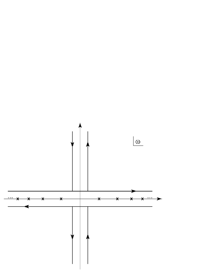
Figure 1: Contours $C_{\underline{\overline{\,\,\,\,}}}$, $C_{\sqcap}$ and $C_{\sqcup}$ on the complex $\omega$-plane; the positions of poles of $G(\omega)$ are indicated by crosses.

and contour $C_{\underline{\overline{\,\,\,\,}}}$ on the complex $\omega$-plane consists of two parallel infinite lines going closely on the lower and upper sides of the real axis, see Fig.1. By deforming the parts of contour $C_{\underline{\overline{\,\,\,\,}}}$ into contours $C_{\sqcap}$ and $C_{\sqcup}$ enclosing the lower and upper imaginary semiaxes, see Fig.1, we get

$$\int\limits_{C_{\underline{\overline{\,\,\,\,}}}}{\rm d}\omega{f(\omega^{2})}G(\omega)=\int\limits_{C_{\sqcap}}{\rm d}\omega{f(\omega^{2})}G(\omega)+\int\limits_{C_{\sqcup}}{\rm d}\omega{f(\omega^{2})}G(\omega),$$

where it is implied that all singularities of $f$ as a function of complex variable $\omega$ lie on the imaginary axis at some distances from the origin. In view of obvious relation

$$\lim\limits_{k\rightarrow{0+}}(k\pm{{\rm i}\kappa})^{2}=\lim\limits_{k\rightarrow{0+}}(-k\mp{{\rm i}\kappa})^{2}=(\pm{{\rm i}\kappa})^{2}$$

for real positive $k$ and $\kappa$, the right-hand side of (B.5) is rewritten in the following way:

$$\int\limits_{C_{\underline{\overline{\,\,\,\,}}}}{\rm d}\omega{f(\omega^{2})}G(\omega)={\rm i}\int\limits_{0}^{\infty}{\rm{d}}\kappa\{f[(-{\rm i}\kappa)^{2}]-f[({\rm i}\kappa)^{2}]\}[G(-{\rm i}\kappa)-G({\rm i}\kappa)].$$

Taking account for relation

$$G(-{\rm i}\kappa)+G({\rm i}\kappa)=2,$$

we further obtain

$$\int\limits_{C_{\underline{\overline{\,\,\,\,}}}}{\rm d}\omega{f(\omega^{2})}G(\omega)=2{\rm i}\int\limits_{0}^{\infty}{\rm{d}}\kappa\{f[(-{\rm i}\kappa)^{2})]-f[({\rm i}\kappa)^{2})]\}G(-{\rm i}\kappa)$$

$$-2{\rm i}\int\limits_{0}^{\infty}{\rm{d}}{\kappa}f[(-{\rm i}\kappa)^{2})]+2{\rm i}\int\limits_{0}^{\infty}{\rm{d}}{\kappa}f[({\rm i}\kappa)^{2})].$$

By rotating the paths of integration in the last and before the last integrals in (B.8) by $90^{\circ}$ in the clockwise and anticlockwise directions, respectively, we finally get

$$\int\limits_{C_{\underline{\overline{\,\,\,\,}}}}{\rm d}\omega{f(\omega^{2})}G(\omega)=2{\rm i}\int\limits_{0}^{\infty}{\rm{d}}\kappa\{f[(-{\rm i}\kappa)^{2})]-f[({\rm i}\kappa)^{2})]\}G(-{\rm i}\kappa)+4\int\limits_{0}^{\infty}{\rm{d}}kf(k^{2}).$$

Note that the explicit form of function $G(\omega)$ is

$$G(\omega)=\frac{(\omega\cosh\vartheta+{\rm i}m){\rm e}^{-{\rm i}{\omega}a}-{\rm i}m\frac{\sin({\omega}a)}{{\omega}a}}{{\omega}\cosh\vartheta\cos({\omega}a)+m\sin({\omega}a)}.$$

Since the numerator of $G(\omega)$ (B.10) contributes to the integral on the left-hand side of (B.9) at values $\omega=k_{l}$ only, one may change the numerator with the use of relation (B.1). We can employ this arbitrariness and change $G(\omega)$ to $\tilde{G}(\omega)$ in such a way that $\tilde{G}(-{\rm i}\kappa)$ will become exponentially decreasing at large values of $\kappa$. Namely, we make substitution

$$m\frac{\sin({\omega}a)}{{\omega}a}\rightarrow-\frac{m^{2}}{{\omega}^{2}\cosh^{2}\vartheta+m^{2}}\,\frac{\cosh\vartheta}{a\cos({\omega}a)}.$$

However, then additional simple poles appear at $\omega=0$ and at $\cos({\omega}a)=0$. Subtracting the contribution of these poles, we obtain

$$\int\limits_{C_{\underline{\overline{\,\,\,\,}}}}{\rm d}\omega{f(\omega^{2})}G(\omega)=2{\rm i}\int\limits_{0}^{\infty}{\rm{d}}\kappa\{f[(-{\rm i}\kappa)^{2})]-f[({\rm i}\kappa)^{2})]\}\tilde{G}(-{\rm i}\kappa)+4\int\limits_{0}^{\infty}{\rm{d}}kf(k^{2})$$

$$-\frac{\rm i}{a}\int\limits_{C_{\underline{\overline{\,\,\,\,}}}}{\rm d}\omega\frac{f(\omega^{2})}{\omega}+\frac{m\cosh\vartheta}{a}\int\limits_{C_{\underline{\overline{\,\,\,\,}}}}{\rm d}\omega\frac{f(\omega^{2})}{{\omega}^{2}\cosh^{2}\vartheta+m^{2}}\frac{{\rm e}^{-{\rm i}{\omega}a}}{\cos({\omega}a)},$$

where

$$\tilde{G}(\omega)=\frac{(\omega\cosh\vartheta+{\rm i}m){\rm e}^{-{\rm i}{\omega}a}+\frac{{\rm i}m^{2}}{{\omega}^{2}\cosh^{2}\vartheta+m^{2}}\,\frac{\cosh\vartheta}{a\cos({\omega}a)}}{{\omega}\cosh\vartheta\cos({\omega}a)+m\sin({\omega}a)}.$$

The last integral on the right-hand side of (B.12) is transformed into integrals along the imaginary axis on the complex $\omega$-plane in the same manner as previously, see (B.5)-(B.9). In this way we get

$$\int\limits_{C_{\underline{\overline{\,\,\,\,}}}}{\rm d}\omega{f(\omega^{2})}G(\omega)=4{\rm i}\int\limits_{0}^{\infty}{\rm{d}}\kappa\{f[(-{\rm i}\kappa)^{2})]-f[({\rm i}\kappa)^{2})]\}\Lambda(\kappa)+4\int\limits_{0}^{\infty}{\rm{d}}kf(k^{2})$$

$$-\frac{2\pi}{a}f(0)+4\frac{m\cosh\vartheta}{a}\int\limits_{0}^{\infty}{\rm{d}}k\frac{f(k^{2})}{k^{2}\cosh^{2}\vartheta+m^{2}},$$

where the contribution of the pole at $\omega=0$ is explicitly written, and

$$\Lambda(\kappa)=\frac{1}{2}\biggl{[}\tilde{G}(-{\rm i}\kappa)-\frac{1}{a}\,\,\frac{m\cosh\vartheta}{\kappa^{2}\cosh^{2}\vartheta-m^{2}}\,\,\frac{{\rm e}^{-{\kappa}a}}{\cosh({\kappa}a)}\biggr{]}$$

is explicitly given by (81). It should be noted that the contribution of poles on the imaginary axis at $\omega=\pm{\rm i}m/\cosh\vartheta$, stemming from substitution (B.11), is canceled. Recalling (B.3), we rewrite (B.14) into the form given by (80).

References

[1] H.B.G.Casimir, Proc. Kon. Ned. Akad. Wetenschap
B51, 793 (1948),
[14]
G.V.Dunne, ’Heisenberg-Euler effective lagrangians: Basics and
extensions’. In: Ian Kogan Memorial Collection ’From Fields
to Strings: Circumnavigating Theoretical Physics’. Ed. by
M.Shifman, A.Vainshtein and J.Wheater (World Scientific,
Singapore, 2004) Vol.1, pp. 445-522.
[15]
J.von Neumann, Mathematische Grundlagen der Quantummechanik
(Springer, Berlin, 1932).
[16]
N.I.Akhiezer and I.M.Glazman, Theory of Linear Operators in
Hilbert Space. Vol. 2 (Pitman, Boston, 1981).
[17]
K.Johnson, Acta Phys. Pol. B6, 865 (1975).
[18]
P.Hasenfratz and J.Kuti, Phys. Rep.40 C, 75 (1978).
[19] M.V.Cougo-Pinto, C.Farina and A.C.Tort, Braz. J. Phys.31, 84 (2001).
[20] E.Elizalde, F.C.Santos and A.C.Tort, J. Phys. A: Math. Theor.35, 7403 (2002).
[25]
A.R.Akhmerov and C.W.J.Beenakker, Phys. Rev. B77,
085423 (2008).
[26]
A.I.Akhiezer and V.B.Berestetskij, Quantum Electrodynamics
(Interscience, New York, 1965).
[27]
A.A.Saharian, ’Generalized Abel-Plana formula as a renormalization
tool in quantum field theory with boundaries’. In: Proc. of
the Fifth Intern. Conf. on Mathematical Methods in Physics. Ed.
by A.A.Bytsenko et al. Proceedings of Science 019-1 - 15 (2006).
[28]
S.Bellucci and A.A.Saharian, Phys. Rev. D80, 105003
(2009).
[29]
L.H.Ford, Phys. Rev. D21, 933 (1980).
[30]
Yu.A.Sitenko and S.A.Yushchenko, Intern. J. Mod. Phys. A29, 1450052 (2014).
[31]
A.K.Harding and D.Lai, Rep. Progr. Phys.69, 2631 (2006).
[33]
J.A.A.J.Perenboom, J.C.Maan, M.R.van Breukelen, S.A.J.Wiegers, A.den Ouden, C.A.Wulfers, W.J.van der Zande, R.T.Jongma, A.F.G.van der Meer and B.Redlich, J. Low Temp. Phys.170, 520 (2013).