Semiclassical spectral function for matter waves in random potentials

Abstract

An $\hbar$-expansion is presented for the ensemble-averaged spectral function of noninteracting matter waves in random potentials. We obtain the leading quantum corrections to the deep classical limit at high energies by the Wigner-Weyl formalism. The analytical results are checked with success against numerical data for Gaussian and laser speckle potentials with Gaussian spatial correlation in two dimensions.

Keywords: Semiclassical theories and applications, matter waves, stochastic processes, transport processes, localisation effects

1 Introduction

With this paper, we present a semiclassical calculation of the spectral function that describes the joint energy-momentum distribution of noninteracting (matter) waves in random potentials. This study has a twofold motivation, theoretical as well as experimental. On the theoretical side, it is a challenge in itself to obtain ensemble-averaged results by semiclassical expansions in strongly disordered systems. The generic case we study in detail is a quantum particle in a smooth, Gaussian random process, a well-known model for benchmarking different approximations [1]. On the experimental side, the dynamics of quantum particles in random potentials is nowadays studied quite intensely with ultracold atoms in random optical potentials, as reviewed in [2, 3, 4]. Two issues under current scrutiny are the distinction between classical diffusion and Anderson localisation [5, 6, 7, 8], and the determination of the mobility edge in laser speckle potentials [9, 10]. These potentials are a well-controlled source of disorder with interesting statistical properties that differ from the simple Gaussian processes mentioned above [11, 12, 13]. Practically, one has to know the spectral function precisely in order to connect the experimentally observed momentum-space densities to characteristic energies. In the strong-disorder regime, analytical weak-disorder approximations cannot be applied. Moreover, trustworthy numerical estimates cost considerable computational resources, especially in two- and three-dimensional settings. Thus, we propose to study the spectral function in strong disorder potentials by a systematic semiclassical expansion around the classical solution.

The rest of the article is structured as follows. Section 2 introduces the spectral function and its properties relevant in the present context, together with the ensemble-averaged density of states. We define the classical limit and show why the usual weak-disorder approximations are inadequate. In Section 3 we provide the computational framework for the leading quantum corrections, at least for the so-called Wigner-Weyl or smooth contribution of point-like periodic orbits. The resulting formula is tested against numerical data for the spectral function in a generic 2d Gaussian potential in Section 4, and in a laser speckle potential in Section 5. We find excellent agreement for the Gaussian case, but also observe that the most salient quantum corrections for red- and especially blue-detuned speckle potentials are beyond the Wigner-Weyl approach. Section 6 summarises.

2 Spectral function

We define the spectral function for matter waves in random potentials, describe a few of its properties, and discuss the limitations of standard weak-disorder approximations.

2.1 Definitions, properties

We consider single-particle systems where the Hamiltonian generator of time evolution, $H({\boldsymbol{r}},{\boldsymbol{p}})=T({\boldsymbol{p}})+V({\boldsymbol{r}})$, is the sum of kinetic and potential energy. In particular, let $V({\boldsymbol{r}})$ be a random potential for the real-space coordinate vector ${\boldsymbol{r}}\in[0,L]^{d}=:L^{d}$ confined to a $d$-dimensional cubic volume. $T({\boldsymbol{p}})$ denotes the kinetic energy, a function of the canonically conjugate momentum of the particle with mass $m$. While our results pertain to arbitrary $T({\boldsymbol{p}})$, we will use the Galilean free-space dispersion $T({\boldsymbol{p}})={\boldsymbol{p}}^{2}/2m$ in concrete examples, and often use the index notation $T_{\boldsymbol{p}}$.

Heisenberg’s commutation relation imposes $[\hat{\boldsymbol{r}},\hat{\boldsymbol{p}}]=\mathrm{i}\hbar$ for the quantum mechanical observables. Since potential and kinetic energy do not commute, neither position nor momentum are good quantum numbers. One possibility to describe the system is by a numerical diagonalisation of the random Hamiltonian for each realisation of disorder, followed by an ensemble average, noted $\overline{(.)}$. However, this procedure can be very costly in terms of computational resources, especially for high-dimensional, strongly disordered systems that require many realisations to reach convergence. Analytical approaches rather try to describe ensemble-averaged quantities from the start. One such quantity, the simplest in some sense, is the average single-particle resolvent $\overline{\hat{G}}(z)=\overline{[z-\hat{H}]^{-1}}$, which is the object of the present work.

We will assume throughout that the disorder potential is statistically homogeneous, meaning that the ensemble average restores translation invariance. Consequently, momentum does become a good quantum number for the average resolvent, whose matrix elements define the single-particle Green function $\langle{\boldsymbol{k}}|\overline{\hat{G}(z)}|{\boldsymbol{k}}^{\prime}\rangle=\delta_{{\boldsymbol{k}}{\boldsymbol{k}}^{\prime}}\overline{G}_{{\boldsymbol{k}}}(z)$. By virtue of its analytical properties, the Green function at any point $z$ in the complex energy plane,

$$\overline{G}_{\boldsymbol{k}}(z)=\int\mathrm{d}E\frac{A_{\boldsymbol{k}}(E)}{z-E},$$ (1)

can be reconstructed from its imaginary part on the real axis, $A_{\boldsymbol{k}}(E)=-\frac{1}{\pi}\mathrm{Im}\lim_{\epsilon\to 0}\overline{G}_{\boldsymbol{k}}(E+\mathrm{i}\epsilon)$. The latter function is known as the spectral function and contains vital information about the (averaged) spectrum of the system. With help of the identity $\mathrm{Im}(x-\mathrm{i}0)^{-1}=\pi\delta(x)$ for the Dirac distribution, it can be written

$$A_{\boldsymbol{k}}(E)=\langle{\boldsymbol{k}}|\overline{\delta(E-\hat{H})}|{\boldsymbol{k}}\rangle.$$ (2)

It thus appears as the probability density that a plane-wave state $|{\boldsymbol{k}}\rangle$ has energy $E$. In the absence of a potential, the spectral function $A_{\boldsymbol{k}}(E)\stackrel{{\scriptstyle V=0}}{{\mapsto}}\delta(E-T_{\boldsymbol{k}})$ projects onto the free dispersion. As a rule, the stronger the perturbation, the broader this function becomes.

Summing over all states yields the average density of states (AVDOS),

$$\nu(E)=\mathrm{tr}\hat{A}(E)=\sum_{\boldsymbol{k}}A_{\boldsymbol{k}}(E),$$ (3)

as the trace of the spectral operator $\hat{A}(E)=\overline{\delta(E-\hat{H})}$. (Sums over momenta are understood to run over ${\boldsymbol{k}}=\hbar{\boldsymbol{n}}/2\pi L$, ${\boldsymbol{n}}\in\mathbbm{Z}^{d}$ allowed by periodic boundary conditions on $[0,L]^{d}$. Note that several conventions for the spectral function exist in the literature, with factors of $2\pi$ in different places—see, e.g., [11, 14] for an alternative.) The definition (2) implies the normalisation

$$\int\mathrm{d}EA_{\boldsymbol{k}}(E)=1.$$ (4)

This relation is but the first out of a hierachy of sum rules reading

$$a^{p}_{\boldsymbol{k}}=\int\mathrm{d}E\,E^{p}A_{\boldsymbol{k}}(E)=\langle{\boldsymbol{k}}|\overline{\hat{H}^{p}}|{\boldsymbol{k}}\rangle.$$ (5)

Apart from the normalisation $a_{\boldsymbol{k}}^{0}=1$, equation (4), we have the first moment $a_{\boldsymbol{k}}^{1}=T_{\boldsymbol{k}}+\overline{V({\boldsymbol{r}})}$. The constant

$$\overline{V({\boldsymbol{r}})}=:\overline{V}$$ (6)

is the average value of the random potential. Other moments of the on-site value are determined by the one-point distribution function $P_{1}(V)$ according to

$$\overline{V^{m}}=\int\mathrm{d}V\,V^{m}P_{1}(V).$$ (7)

Since we assume $V({\boldsymbol{r}})$ to be an ergodic process, ensemble averages can also be obtained by spatial averages $\overline{V^{m}}=L^{-d}\int\mathrm{d}{\boldsymbol{r}}V({\boldsymbol{r}})^{m}$. (Integrals over positions are understood to run over the volume $[0,L]^{d}$.)

With the second moment,

$$a^{2}_{\boldsymbol{k}}=\left(T_{\boldsymbol{k}}+\overline{V}\right)^{2}+\overline{\delta V({\boldsymbol{r}})^{2}}.$$ (8)

on-site fluctuations around the mean, $\delta V({\boldsymbol{r}})=V({\boldsymbol{r}})-\overline{V}$, come into play. Their second moment, $\overline{\delta V({\boldsymbol{r}})^{2}}=:\delta V^{2}$, measures the on-site variance of potential fluctuations.

Starting from the third moment $a^{3}_{\boldsymbol{k}}$, also information about spatial correlations between fluctuations is encoded. In the remainder of this work, we will only require the covariance

$$\overline{\delta V({\boldsymbol{r}})\delta V({\boldsymbol{r}}^{\prime})}=\delta V^{2}C({\boldsymbol{r}}-{\boldsymbol{r}}^{\prime}).$$ (9)

Typically, the correlation function $C({\boldsymbol{r}})$ decays from 1 to 0 over a microscopic length scale $\zeta$ (for notational simplicity, we consider isotropic correlations). This introduces a correlation energy scale, $E_{\zeta}=\hbar^{2}/m\zeta^{2}$. In the following, we will focus exclusively on the strong-potential regime defined by

$$\delta V\gg E_{\zeta}.$$ (10)

In this situation, the atom kinetic energy fluctuates also by $\delta T(k)\sim\delta V\gg E_{\zeta}$, and therefore produces large momenta $k\gg\hbar/\zeta$. In other words, the dynamics of matter waves inside the random potential will be dominated by the semiclassical regime $k\zeta\gg\hbar$.

In the following two sections, limiting cases are discussed where analytical results are known, namely the weak-disorder limit and the deep classical limit.

2.2 Self-energy and inadequacy of Born approximations

In the semiclassical regime, standard weak-disorder approximations [15, 11, 16, 17] prove to be inadequate. The weak-disorder estimates try to construct the spectral function from the information contained in the lowest moments of the random potential, mean (6) and covariance (9). This is most economically achieved by introducing the self-energy $\Sigma_{\boldsymbol{k}}(z)$ via Dyson’s equation $\overline{G}_{\boldsymbol{k}}(z)=[z-T_{\boldsymbol{k}}-\Sigma_{\boldsymbol{k}}(z)]^{-1}$ and taking the limit $z=E+\mathrm{i}0$. The spectral function then is

$$A_{\boldsymbol{k}}(E)=-\frac{1}{\pi}\frac{\mathrm{Im}\Sigma_{\boldsymbol{k}}(E)}{[E-{T_{\boldsymbol{k}}}-\mathrm{Re}\Sigma_{\boldsymbol{k}}(E)]^{2}+\mathrm{Im}\Sigma_{\boldsymbol{k}}(E)^{2}}.$$ (11)

Formal operator identities permit to expand the self-energy in an asymptotic series,

$$\Sigma_{\boldsymbol{k}}(z)=\overline{V}+\langle{\boldsymbol{k}}|\left(\overline{\hat{V}(z-\hat{T})^{-1}\hat{V}}-\overline{V}(z-\hat{T})^{-1}\overline{V}\right)|{\boldsymbol{k}}\rangle+\dots$$ (12)

involving only connected averages of the potential. The first term merely shifts the energy by the potential mean. The second term contains information about the variance. If the series is truncated after this term, it results in the so-called Born approximation (BA),

$$\Sigma^{\text{BA}}_{\boldsymbol{k}}(z)=\overline{V}+\sum_{{\boldsymbol{k}}^{\prime}}\frac{\overline{|\delta V_{{\boldsymbol{k}}-{\boldsymbol{k}}^{\prime}}|^{2}}}{z-T_{{\boldsymbol{k}}^{\prime}}}=\overline{V}+\delta V^{2}\sum_{{\boldsymbol{k}}^{\prime}}\frac{C_{{\boldsymbol{k}}-{\boldsymbol{k}}^{\prime}}}{z-T_{{\boldsymbol{k}}^{\prime}}}$$ (13)

where $\delta V_{{\boldsymbol{k}}-{\boldsymbol{k}}^{\prime}}=\langle{\boldsymbol{k}}|\delta\hat{V}|{\boldsymbol{k}}^{\prime}\rangle=L^{-d}\int\rmd{\boldsymbol{r}}e^{-i({\boldsymbol{k}}-{\boldsymbol{k}}^{\prime})\cdot{\boldsymbol{r}}}\delta V({\boldsymbol{r}})$ is the Fourier component of the potential fluctuation. The second equality of Eq. (13) introduces the Fourier transform

$$C_{\boldsymbol{k}}=L^{-d}\int\mathrm{d}{\boldsymbol{r}}e^{-\mathrm{i}{\boldsymbol{k}}{\boldsymbol{r}}}C({\boldsymbol{r}})=\overline{\delta V_{\boldsymbol{k}}\delta V_{\boldsymbol{k}}^{*}}/\delta V^{2}$$ (14)

of the real-space correlator (9), normalised to $\sum_{\boldsymbol{k}}C_{\boldsymbol{k}}=1$.

Since the BA (13) neglects terms of order $\delta V^{3}$, it can hold only for weak potential fluctuations compared to the other energies involved, $\delta V^{2}\ll TE_{\zeta}$ [11]. A popular extension that pretends to a larger range of validity is the self-consistent BA (SCBA), where the free propagator in (13) is replaced by the renormalised propagator itself,

$$\Sigma^{\text{SCBA}}_{\boldsymbol{k}}(z)=\overline{V}+\delta V^{2}\sum_{{\boldsymbol{k}}^{\prime}}\frac{C_{{\boldsymbol{k}}-{\boldsymbol{k}}^{\prime}}}{z-T_{{\boldsymbol{k}}^{\prime}}-\Sigma^{\text{SCBA}}_{{\boldsymbol{k}}^{\prime}}(z)}.$$ (15)

This equation has to be solved numerically for the unknown complex function $\Sigma^{\text{SCBA}}_{\boldsymbol{k}}(z)$ appearing on both sides. Despite its popularity, the SCBA fails badly in the semiclassical regime of interest. Indeed, define $z_{\boldsymbol{k}}:=(z-T_{\boldsymbol{k}}-\overline{V})/\delta V$ as well as $\sigma_{\boldsymbol{k}}(z):=(\Sigma_{\boldsymbol{k}}(z)-\overline{V})/\delta V$ and consider (15) in the formal limit $\hbar\to 0$ (i.e., $\delta V/E_{\zeta}\to\infty$). Since the correlation function $C_{{\boldsymbol{k}}-{\boldsymbol{k}}^{\prime}}$ constrains $|{\boldsymbol{k}}-{\boldsymbol{k}}^{\prime}|$ to be of order $\hbar/\zeta$, it turns into $\delta_{{\boldsymbol{k}}{\boldsymbol{k}}^{\prime}}$. The scaled complex self-energy $\sigma_{\boldsymbol{k}}=\sigma^{\prime}_{\boldsymbol{k}}+\mathrm{i}\sigma^{\prime\prime}_{\boldsymbol{k}}$ then obeys the self-consistent equation $\sigma_{\boldsymbol{k}}=(z_{\boldsymbol{k}}-\sigma_{\boldsymbol{k}})^{-1}$. This can be readily solved for the real and imaginary parts, $\sigma^{\prime}_{\boldsymbol{k}}=z_{\boldsymbol{k}}/2$ and $\sigma_{\boldsymbol{k}}^{\prime\prime}=-[1-(z_{\boldsymbol{k}}-\sigma_{\boldsymbol{k}}^{\prime})^{2}]^{1/2}=-\sqrt{1-z_{\boldsymbol{k}}^{2}/4}$. As a consequence, the spectral density (11) becomes

$$A_{\boldsymbol{k}}^{\text{SCBA}}(E)=\frac{1}{\pi\delta V}\sqrt{1-\frac{(E-\overline{V}-T_{\boldsymbol{k}})^{2}}{4\delta V^{2}}},\qquad(\hbar\to 0),$$ (16)

where $|E-\overline{V}-T_{\boldsymbol{k}}|\leq 2\delta V$, and vanishes elsewhere. In a zero-dimensional setting where the kinetic energy is irrelevant, this form of the resulting AVDOS is known as “Wigner’s semi-circle law,” a celebrated property of random-matrix ensembles [18, 19]. However, this ‘universal’ law generally lies far from the true result in the deep classical limit, discussed next.

2.3 Classical limit

One may neglect the non-commutativity of $\hat{\boldsymbol{r}}$ and $\hat{\boldsymbol{p}}$ entirely in the deep classical limit $\delta V/E_{\zeta}\to\infty$ that is noted commonly, if rather abusively, $\hbar\to 0$. In this limit, sometimes referred to as the Thomas-Fermi limit [20], the expectation value

$$\langle{\boldsymbol{k}}|\overline{\delta(E-\hat{H})}|{\boldsymbol{k}}\rangle\stackrel{{\scriptstyle\hbar\to 0}}{{\to}}\overline{\delta(E-T_{\boldsymbol{k}}-V_{1})}$$ (17)

depends only on the potential value $V_{1}=V({\boldsymbol{r}}_{1})$ at an arbitrary point ${\boldsymbol{r}}_{1}$. Then the ensemble average $\overline{\delta(x-V_{1})}=\int\mathrm{d}V_{1}\delta(x-V_{1})P_{1}(V_{1})=P_{1}(x)$ produces the spectral function

$$A_{{\boldsymbol{k}}}^{\text{cl}}(E)=P_{1}(E-T_{{\boldsymbol{k}}}).$$ (18)

The corresponding AVDOS (3) is

$$\nu^{\text{cl}}(E)=\sum_{\boldsymbol{k}}P_{1}(E-T_{\boldsymbol{k}})=\int\rmd T\nu_{0}(T)P_{1}(E-T),$$ (19)

namely the convolution of the free DOS $\nu_{0}(E)$ with the one-point distribution [20, 13]. For the Galilean dispersion, one has $\nu_{0}(E)=N_{d}E^{(d-2)/2}\Theta(E)$, with $N_{d}$ a constant proportional to the $d$-dimensional volume of the system.

The exact result (18) means that in the deep classical limit, the probability for a particle with momentum ${\boldsymbol{k}}$ to have potential energy $V=E-T_{\boldsymbol{k}}$ is given by the on-site distribution $P_{1}(V)$ alone [21]. This distribution need not be close to the semi-circle law of the SCBA result, Eq. (16). Moreover, for certain classes of potentials such as the laser speckle potentials discussed in section 5 below, the distribution function is not even. Then, there can be no hope to catch the strong-disorder properties of the spectral function by an approximation like SCBA that is built solely upon even powers of the fluctuations, and a systematic description of quantum corrections beyond the classical limit is desirable. Quantum corrections to this classical limit arise because finite (in the sense of less-than-infinite) momenta probe nonlocal features of the potential and thus should be sensitive to its correlations. Accordingly, the classical limit (18) obeys the first three sum rules for $p=0,1,2$ already on its own, and quantum corrections can only be expected to arise for higher-oder sum rules $p\geq 3$, which are sensitive to the spatial correlations. The systematic semiclassical derivation of such corrections is the subject of the next section.

3 Semiclassical corrections

With this section, we turn to the calculation of quantum corrections

$$\Delta A_{\boldsymbol{k}}(E)=A_{\boldsymbol{k}}(E)-A^{\text{cl}}_{\boldsymbol{k}}(E)$$ (20)

to the deep classical limit (18). The proper tool in the regime of interest, $\delta V\gg E_{\zeta}$, is a semiclassical approximation. We face the task of computing the (momentum-)local average density of states,

$$A_{{\boldsymbol{k}}}(E)=\mathrm{tr}\{|{\boldsymbol{k}}\rangle\langle{\boldsymbol{k}}|\overline{\delta(E-\hat{H})}\}.$$ (21)

The calculation of traces like this has a long-standing history in semiclassical physics, where phase-coherent quantum evolution is described by the superposition of Feynman path amplitudes. Two types of contributions to formal $\hbar$-expansions around the classical solution are known [22, 23]: first the so-called smooth part, also known as Wigner-Weyl corrections, formally due to orbits of zero length, and second the so-called fluctuating part, due to periodic orbits of finite length. The present paper is devoted to the calculation of the smooth Wigner-Weyl corrections. The importance of periodic-orbit contributions is discussed in the concluding section 6.

3.1 Semiclassical expression for the spectral function

In order to compute the quantum corrections to the smooth part, we employ Wigner’s phase space formulation of quantum mechanics [24, 25, 26, 27, 28, 29, 30] in notations adapted to a finite-size system with discrete momenta [31, 32]. In this formalism, the trace of an arbitrary operator $X(\hat{{\boldsymbol{r}}},\hat{{\boldsymbol{p}}})$ is expressed as the phase-space integral

$$\mathrm{tr}\{X(\hat{{\boldsymbol{r}}},\hat{{\boldsymbol{p}}})\}=\frac{1}{L^{d}}\sum_{{\boldsymbol{p}}}\int\mathrm{d}{\boldsymbol{r}}\,X_{W}({\boldsymbol{r}},{\boldsymbol{p}})$$ (22)

over its Wigner function

$$X_{W}({\boldsymbol{r}},{\boldsymbol{p}}) =\int\mathrm{d}{\boldsymbol{r}}^{\prime}\,e^{\mathrm{i}{\boldsymbol{p}}{\boldsymbol{r}}^{\prime}/\hbar}\langle{\boldsymbol{r}}-\frac{{\boldsymbol{r}}^{\prime}}{2}|X(\hat{{\boldsymbol{r}}},\hat{{\boldsymbol{p}}})|{\boldsymbol{r}}+\frac{{\boldsymbol{r}}^{\prime}}{2}\rangle$$ (23)

$$=\sum_{{\boldsymbol{q}}}e^{-2\mathrm{i}{\boldsymbol{q}}{\boldsymbol{r}}/\hbar}\langle{\boldsymbol{p}}-{\boldsymbol{q}}|X(\hat{{\boldsymbol{r}}},\hat{{\boldsymbol{p}}})|{\boldsymbol{p}}+{\boldsymbol{q}}\rangle.$$ (24)

The function $X_{W}({\boldsymbol{r}},{\boldsymbol{p}})$, also called Wigner transform or Weyl symbol [33] can equivalently be written as the scalar product $X_{W}({\boldsymbol{r}},{\boldsymbol{p}})=\mathrm{tr}\{X(\hat{{\boldsymbol{r}}},\hat{{\boldsymbol{p}}})W(\hat{{\boldsymbol{r}}}-{\boldsymbol{r}};\hat{\boldsymbol{p}}-{\boldsymbol{p}})\}$ with the Stratonovich-Weyl operator kernel

$$W(\hat{{\boldsymbol{r}}}-{\boldsymbol{r}};\hat{\boldsymbol{p}}-{\boldsymbol{p}}) =\exp\left(-\frac{2\mathrm{i}}{\hbar}(\hat{{\boldsymbol{r}}}-{\boldsymbol{r}});(\hat{{\boldsymbol{p}}}-{\boldsymbol{p}})\right)$$ (25)

$$=\int\mathrm{d}{\boldsymbol{r}}^{\prime}\,e^{\mathrm{i}{\boldsymbol{p}}{\boldsymbol{r}}^{\prime}/\hbar}|{\boldsymbol{r}}+\frac{{\boldsymbol{r}}^{\prime}}{2}\rangle\langle{\boldsymbol{r}}-\frac{{\boldsymbol{r}}^{\prime}}{2}|$$ (26)

$$=\sum_{{\boldsymbol{q}}}e^{-2\mathrm{i}{\boldsymbol{q}}{\boldsymbol{r}}/\hbar}|{\boldsymbol{p}}+{\boldsymbol{q}}\rangle\langle{\boldsymbol{p}}-{\boldsymbol{q}}|.$$ (27)

The semicolon in (25) indicates ordering of products of $\hat{{\boldsymbol{r}}}$ and $\hat{{\boldsymbol{p}}}$ such that $\hat{{\boldsymbol{r}}}$ always stands left of $\hat{{\boldsymbol{p}}}$. Since this kernel obeys the Hilbert-Schmidt orthogonality

$$\mathrm{tr}\{W(\hat{{\boldsymbol{r}}}-{\boldsymbol{r}};\hat{\boldsymbol{p}}-{\boldsymbol{p}})W(\hat{{\boldsymbol{r}}}-{\boldsymbol{r}}^{\prime};\hat{\boldsymbol{p}}-{\boldsymbol{p}}^{\prime})\}=\delta({\boldsymbol{r}}-{\boldsymbol{r}}^{\prime})\,L^{d}\,\delta_{{\boldsymbol{p}},{\boldsymbol{p}}^{\prime}}\ ,$$ (28)

one can invert (23) and write the operator in terms of its Wigner function,

$$X(\hat{{\boldsymbol{r}}},\hat{{\boldsymbol{p}}})=\frac{1}{L^{d}}\sum_{{\boldsymbol{p}}}\int\mathrm{d}{\boldsymbol{r}}\,X_{W}({\boldsymbol{r}},{\boldsymbol{p}})\,W(\hat{{\boldsymbol{r}}}-{\boldsymbol{r}};\hat{\boldsymbol{p}}-{\boldsymbol{p}})\ .$$ (29)

Moreover, it follows that the trace of a product of operators $X(\hat{{\boldsymbol{r}}},\hat{{\boldsymbol{p}}})$ and $Y(\hat{{\boldsymbol{r}}},\hat{{\boldsymbol{p}}})$ is the phase-space integral of their Wigner function product:

$$\mathrm{tr}\{\hat{X}\,\hat{Y}\}=\frac{1}{L^{d}}\sum_{{\boldsymbol{p}}}\int\mathrm{d}{\boldsymbol{r}}\,X_{W}({\boldsymbol{r}},{\boldsymbol{p}})\,Y_{W}({\boldsymbol{r}},{\boldsymbol{p}})\ .$$ (30)

Applied to (21) with $\hat{X}=|{\boldsymbol{k}}\rangle\langle{\boldsymbol{k}}|$ and $\hat{Y}=\delta(E-\hat{H})$ before the ensemble average, this yields

$$\mathrm{tr}\{|{\boldsymbol{k}}\rangle\langle{\boldsymbol{k}}|\delta(E-\hat{H})\} =\frac{1}{L^{d}}\int\mathrm{d}{\boldsymbol{r}}\,[\delta(E-\hat{H})]_{W}({\boldsymbol{r}},{\boldsymbol{k}})$$ (31)

since $|{\boldsymbol{k}}\rangle\langle{\boldsymbol{k}}|_{W}({\boldsymbol{r}},{\boldsymbol{p}})=\delta_{{\boldsymbol{k}}{\boldsymbol{p}}}$ projects onto the momentum ${\boldsymbol{k}}$. Upon the ensemble average, the argument under the integral becomes independent of ${\boldsymbol{r}}$, and we thus arrive at the first result

$$A_{\boldsymbol{k}}(E)=\overline{\delta(E-\hat{H})_{W}}({\boldsymbol{k}})\ .$$ (32)

3.2 Semiclassical expansion to order $\hbar^{2}$

This previous result (32) is still exact. An approximation becomes necessary for the Wigner transform $\delta(E-\hat{H})_{W}$, which cannot be determined in closed form for arbitrary potentials. But one can compute quantum corrections to leading order in $\hbar$, which are well known [34]:

$$\delta(E-\hat{H})_{W}\approx\delta(E-H)-\frac{\hbar^{2}}{16}\left\{H\overleftrightarrow{\Lambda}{}^{2}H\right\}\delta^{\prime\prime}(E-H)-\frac{\hbar^{2}}{24}\left\{H\overleftrightarrow{\Lambda}H\overleftrightarrow{\Lambda}H\right\}\delta^{\prime\prime\prime}(E-H).$$ (33)

Here, $H=T({\boldsymbol{k}})+V({\boldsymbol{r}})$ is the classical Hamiltonian function. The first term inserted into (32) yields the expected classical result (18). Quantum corrections involve the differential operator

$$\overleftrightarrow{\Lambda}=\overleftarrow{\partial_{{\boldsymbol{r}}}}\cdot\overrightarrow{\partial_{{\boldsymbol{k}}}}-\overleftarrow{\partial_{{\boldsymbol{k}}}}\cdot\overrightarrow{\partial_{{\boldsymbol{r}}}}$$ (34)

that implements the Poisson bracket in linear order, $\{f\overleftrightarrow{\Lambda}g\}=\{f,g\}$. In the second-order terms of (33), $\overleftrightarrow{\Lambda}$ is understood to act only on the directly neighboring functions [35]. The series (33) is obtained as a consequence of the Wigner representation of a product of operators,

$$[AB]_{W}({\boldsymbol{r}},{\boldsymbol{p}})=A_{W}({\boldsymbol{r}},{\boldsymbol{p}})\exp\left[\frac{i\hbar}{2}\overleftrightarrow{\Lambda}\right]B_{W}({\boldsymbol{r}},{\boldsymbol{p}}),$$ (35)

known as the Wigner-Groenewold-Moyal (star) product [24, 25, 26].

For our separable Hamiltonian, we find

$$\big{\{}H\overleftrightarrow{\Lambda}{}^{2}H\big{\}} =2\sum_{i,j=1}^{d}(\partial_{r_{i}}\partial_{r_{j}}V)(\partial_{k_{i}}\partial_{k_{j}}T)\ ,$$ (36)

$$\big{\{}H\overleftrightarrow{\Lambda}H\overleftrightarrow{\Lambda}H\big{\}} =-\sum_{i,j=1}^{d}\left[(\partial_{r_{i}}\partial_{r_{j}}V)(\partial_{k_{i}}T)(\partial_{k_{j}}T)+(\partial_{r_{i}}V)(\partial_{r_{j}}V)(\partial_{k_{i}}\partial_{k_{j}}T)\right].$$ (37)

We remark, moreover, that one may group the second terms from (37), of the type $(\partial V)^{2}\delta^{\prime\prime\prime}(E-H)=-(\partial V)\partial\delta^{\prime\prime}(E-H)$, with the terms of type $(\partial^{2}V)\delta^{\prime\prime}(E-H)$ from (36) by partial integration under the ${\boldsymbol{r}}$-integral in (31). Thus, the leading-order quantum corrections to the spectral function are

$$\Delta A_{{\boldsymbol{k}}}(E)\approx-\frac{\hbar^{2}}{12}\sum_{i,j=1}^{d}\left[m_{ij}^{-1}C_{ij}^{(2)}(\xi)-\frac{v_{i}v_{j}}{2}C_{ij}^{(3)}(\xi)\right].$$ (38)

Here we have introduced the variable

$$\xi:=E-T_{\boldsymbol{k}}$$ (39)

together with the possibly ${\boldsymbol{k}}$-dependent tensors of inverse effective mass $m_{ij}^{-1}=\partial_{k_{i}}\partial_{k_{j}}T_{\boldsymbol{k}}$ and group velocities $v_{i}v_{j}=(\partial_{k_{i}}T_{\boldsymbol{k}})(\partial_{k_{j}}T_{\boldsymbol{k}})$. The ensemble-averaged functions

$$C_{ij}^{(n)}(\xi):=\overline{(\partial_{r_{i}}\partial_{r_{j}}V({\boldsymbol{r}}))\delta^{(n)}(\xi-V({\boldsymbol{r}}))}$$ (40)

remain to be expressed by the statistical properties of the random process $V({\boldsymbol{r}})$.

3.3 Moments from characteristic functional

Expression (40) requires to calculate moments of potential derivatives. This suggests the Fourier representation $V({\boldsymbol{r}})=\sum_{{\boldsymbol{q}}}e^{\mathrm{i}{\boldsymbol{q}}{\boldsymbol{r}}}V_{{\boldsymbol{q}}}$ such that

$$\partial_{r_{i}}\partial_{r_{j}}V({\boldsymbol{r}})=-\sum_{{\boldsymbol{q}}}q_{i}q_{j}e^{\mathrm{i}{\boldsymbol{q}}{\boldsymbol{r}}}V_{{\boldsymbol{q}}}.$$ (41)

(We set $\hbar=1$ in the Fourier expansion since it does not interfere with the formal $\hbar$-expansion.) Similarly, we write the derivatives of Dirac distributions as the Fourier integrals

$$\delta^{(n)}(\xi-V({\boldsymbol{r}}))=\partial_{\xi}^{n}\int\frac{\mathrm{d}\alpha}{2\pi}e^{-\mathrm{i}\alpha[\xi-V({\boldsymbol{r}})]}.$$ (42)

Then, the ensemble average in (40) has to be taken over the combination $\overline{V_{{\boldsymbol{q}}}\,e^{\mathrm{i}\alpha V({\boldsymbol{r}})}}$. We generate the prefactor $V_{\boldsymbol{q}}$ by the differentiation

$$\overline{V_{{\boldsymbol{q}}}\,e^{\mathrm{i}\alpha V({\boldsymbol{r}})}} =-\left.\mathrm{i}\frac{\partial\chi[\beta]}{\partial\beta_{{\boldsymbol{q}}}}\right|_{\beta_{{\boldsymbol{p}}}=\alpha e^{\mathrm{i}{\boldsymbol{p}}{\boldsymbol{r}}}}$$ (43)

of the characteristic functional in the momentum representation,

$$\chi[\beta]=\overline{\exp\mathrm{i}\sum_{{\boldsymbol{p}}}\beta_{{\boldsymbol{p}}}V_{{\boldsymbol{p}}}}.$$ (44)

With the choice $\beta_{\boldsymbol{p}}=\alpha e^{\mathrm{i}{\boldsymbol{p}}{\boldsymbol{r}}}$, it returns

$$\chi[\alpha e^{\mathrm{i}{\boldsymbol{p}}{\boldsymbol{r}}}]=\overline{\exp\mathrm{i}\alpha V({\boldsymbol{r}})}=\int\mathrm{d}Ve^{\mathrm{i}\alpha V}P_{1}(V)=:\chi_{1}(\alpha),$$ (45)

the characteristic function of the one-point distribution. Since the ensemble-averaged result does not depend on the point ${\boldsymbol{r}}$, we may choose ${\boldsymbol{r}}=0$ to simplify notations. Thus, the coefficients (40) become

$$C_{ij}^{(n)}(\xi) =\mathrm{i}\sum_{{\boldsymbol{q}}}q_{i}q_{j}\partial_{\xi}^{n}\int\frac{\mathrm{d}\alpha}{2\pi}e^{-\mathrm{i}\alpha\xi}\left.\frac{\partial\chi[\beta]}{\partial\beta_{{\boldsymbol{q}}}}\right|_{\beta_{{\boldsymbol{p}}}=\alpha}\ .$$ (46)

Here ends the general development of the theory. Once the characteristic functional (44) of a specific random potential is given, one can compute the functions (46) and evaluate (38). This will be carried out in the following two sections for a Gaussian random process and a laser speckle potential, respectively.

4 Gaussian potentials

As a benchmark test for the semiclassical approach we consider a Gaussian random process centered on $\overline{V}=0$ and with variance $V^{2}=\delta V^{2}$.

4.1 Statistical properties

The full distribution functional of the Gaussian random process of interest is

$$P[V] =\mathcal{N}_{1}\exp\left(-\frac{1}{2V^{2}}\sum_{{\boldsymbol{q}}}V_{{\boldsymbol{q}}}^{*}C_{{\boldsymbol{q}}}^{-1}V_{{\boldsymbol{q}}}\right)$$ (47)

with a normalisation constant $\mathcal{N}_{1}$ and the two-point correlation (14). Its characteristic functional is equally Gaussian,

$$\chi[\beta]=\exp\left(-\frac{V^{2}}{2}\sum_{{\boldsymbol{q}}}\beta_{{\boldsymbol{q}}}^{*}\,C_{{\boldsymbol{q}}}\beta_{{\boldsymbol{q}}}\right)\ ,$$ (48)

and the derivative required in (46) reads

$$\left.\frac{\partial\chi[\beta]}{\partial\beta_{{\boldsymbol{q}}}}\right|_{\beta_{{\boldsymbol{p}}}=\alpha}=-V^{2}C_{{\boldsymbol{q}}}\alpha\chi_{1}(\alpha)$$ (49)

with $\chi_{1}(\alpha)=\exp(-V^{2}\alpha^{2}/2)$. The one-point distribution is of course also Gaussian,

$$P_{1}(\xi)=\int\frac{\mathrm{d}\alpha}{2\pi}e^{-\mathrm{i}\alpha\xi}\chi_{1}(\alpha)=(2\pi V^{2})^{-1/2}\exp\left(-\frac{\xi^{2}}{2V^{2}}\right).$$ (50)

4.2 Spectral function

With (49) and (50), the functions (46) become

$$C_{ij}^{(n)}(\xi) =V^{2}C_{ij}P_{1}^{(n+1)}(\xi)$$ (51)

where

$$C_{ij}=\sum_{\boldsymbol{q}}q_{i}q_{j}C_{{\boldsymbol{q}}}=-\partial_{r_{i}}\partial_{r_{j}}C({\boldsymbol{r}})|_{{\boldsymbol{r}}=0}$$ (52)

is the correlation curvature. Combining all factors, we obtain

$$\Delta A_{\boldsymbol{k}}(E)\approx-\frac{\hbar^{2}V^{2}}{12}\!\sum_{i,j=1}^{d}\!C_{ij}\left[m_{ij}^{-1}\partial_{E}^{3}-\frac{v_{i}v_{j}}{2}\partial_{E}^{4}\right]\!P_{1}(E-T_{\boldsymbol{k}}).$$ (53)

With an isotropic dispersion $T_{\boldsymbol{k}}={\boldsymbol{k}}^{2}/2m$ such that $m_{ij}^{-1}=\delta_{ij}/m$ as well as $v_{i}=k_{i}/m$ and an isotropic Gaussian spatial correlation $C({\boldsymbol{r}})=\exp\left[-{\boldsymbol{r}}^{2}/(2\zeta^{2})\right]$ such that $C_{ij}=\delta_{ij}/\zeta^{2}$, this simplifies to

$$\Delta A_{{\boldsymbol{k}}}(E)\approx-\frac{V^{2}E_{\zeta}}{12}\left[d\partial_{E}^{3}-T_{\boldsymbol{k}}\partial_{E}^{4}\right]P_{1}(E-T_{\boldsymbol{k}}).$$ (54)

This correction involves third and fourth derivatives of the one-point potential distribution, a property that ensures that quantum corrections do not change the sum rules (5) at the three lowest orders $p=0,1,2$, which are alread exhausted by the classical limit $A^{\text{cl}}_{\boldsymbol{k}}(E)=P_{1}(E-T_{\boldsymbol{k}})$. The first one to be corrected is the cubic moment, classically given by $a_{\boldsymbol{k}}^{3,\text{cl}}=3V^{2}T_{\boldsymbol{k}}+T_{\boldsymbol{k}}^{3}$ and shifted by $\Delta a_{\boldsymbol{k}}^{3}=dV^{2}E_{\zeta}/2$, actually independent of ${\boldsymbol{k}}$, but governed by the “quantum” energy scale $E_{\zeta}=\hbar^{2}/m\zeta^{2}$.

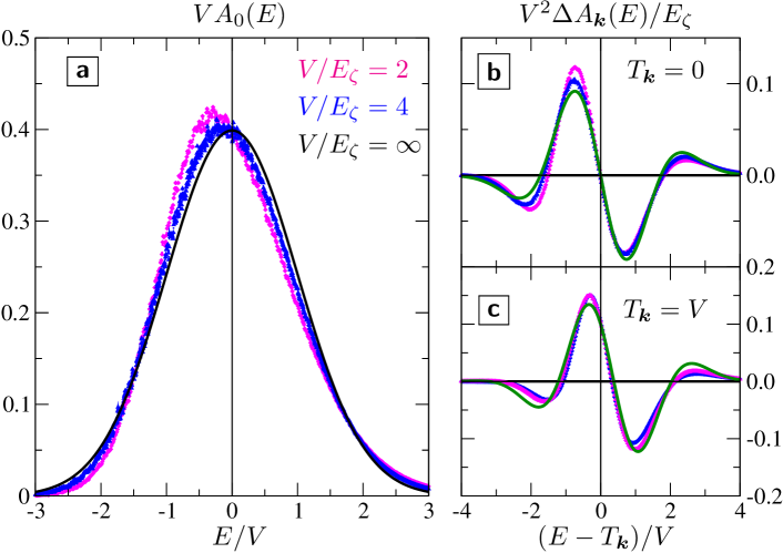
Figure 1: Panel (a): Spectral function $A_{0}(E)$ at zero momentum as function of energy $E$ (in units of rms potential strength $V$) for $V/E_{\zeta}=2,4$ in $d=2$ dimensions, approaching the normal distribution $P_{1}(E)$ (thick black line). Panel (b): The quantum correction $\Delta A_{0}(E)$ in scaled vertical units such that the data collapse onto the semiclassical approximation (55), shown as the continuous green curve on top of the data points. Panel (c): Same plot as in (b), but for finite momentum such that $T_{\boldsymbol{k}}=V$, showing equally good agreement with the prediction (54).

Figure 1 shows in panel (a) $A_{0}(E)$ at zero momentum as function of energy $E$ (both in units of the rms potential strength $V$) for different values of $V/E_{\zeta}$ in $d=2$ dimensions. Data points are the result of a numerical calculation and reproduce results available in the literature [1]; A contains technical details about the numerical methods. The computed data curves converge toward the classical result, the normal distribution $A^{\text{cl}}_{0}(E)=P_{1}(E)$ of eq. (50). In panel (b), we plot the semiclassical approximation for the quantum corrections,

$$\Delta A_{0}(E)\approx-\frac{EE_{\zeta}}{6V^{2}}\left(3-\frac{E^{2}}{V^{2}}\right)P_{1}(E),$$ (55)

which is found to reproduce the data very well. Notably, since the correction is proportional to $P_{1}^{\prime\prime\prime}(E)$, it vanishes at the origin and $E=\pm\sqrt{3}V$ and thus explains the approximate crossing of all curves at these points, for large enough values of $V/E_{\zeta}$. The lowest-order approximation starts to deviate from the data when $V/E_{\zeta}$ becomes too small, but the general trend is captured faithfully down to about $V/E_{\zeta}=2$.

Indeed, since $P_{1}(\xi)=V^{-1}g(\xi/V)$ with a scalar gaussian function $g(x)$ of order unity, the correction (54) scales as $E_{\zeta}/V^{2}$ multiplying another scalar function $h(x)$ of order unity (here a polynomial times $g(x)$). Our formal $\hbar$-expansion is justified ex post if this correction is small, which is the case in the semiclassical regime $E_{\zeta}/V\ll 1$. Therefore, the quality of this approximation is independent of $T_{\boldsymbol{k}}$, as apparent also from panel (c) in Fig. 1, where the deviation is plotted for finite $T_{\boldsymbol{k}}=V$.

4.3 Average density of states

In $d=2$ where $\nu_{0}(E)=N_{2}\Theta(E)$ is a pure step function of energy, the classical AVDOS (19) becomes the integral of the one-point distribution up to $E$. For the normal distribution, this gives the well-known error function,

$$\nu^{\text{cl}}(E)=N_{2}\int_{-\infty}^{E}\rmd TP_{1}(T)=\frac{N_{2}}{2}\left[1+\text{erf}(E/{\sqrt{2}}V)\right],$$ (56)

which smoothens the free DOS around zero energy on the scale $V$. The semiclassical corrections following from (54) in this case take a particularly simple form,

$$\Delta\nu(E)\approx-N_{2}\frac{V^{2}E_{\zeta}}{12}P_{1}^{\prime\prime}(E)=\frac{N_{2}E_{\zeta}}{{12}}\left({1}-\frac{E^{2}}{V^{2}}\right)P_{1}(E),$$ (57)

with a vanishing correction predicted at $|E|=V$.

5 Speckle potentials

Another class of interesting random potentials are laser speckle, relevant for experiments with ultracold atoms [4]. The atoms experience a dipolar light-shift potential $V({\boldsymbol{r}})=s|E({\boldsymbol{r}})|^{2}$ proportional to the local light intensity created by the random electric field $E({\boldsymbol{r}})$. The proportionality factor $s$ encodes the atomic polarisability, besides the necessary dimensionfull constants, and can have either positive or negative sign, for blue- and red-detuned laser light, respectively. In the following, we choose units such that $s=\pm 1$. We first review a few statistical properties and derive the characteristic functional $\chi[\beta]$ needed for the semiclassical corrections.

5.1 Statistical properties

We neglect finite-size and polarisation effects, and suppose that the field $E({\boldsymbol{r}})$ is a scalar, complex, Gaussian random process. Its real-space covariance is

$$\overline{E^{*}({\boldsymbol{r}})E({\boldsymbol{r}}^{\prime})}=\overline{|E|^{2}}\gamma({\boldsymbol{r}}-{\boldsymbol{r}}^{\prime})$$ (58)

with $\gamma(-{\boldsymbol{r}})=\gamma({\boldsymbol{r}})^{*}$ and $\gamma(0)=1$ by definition. Equivalently, the Fourier components $E_{\boldsymbol{p}}=L^{-d}\int\mathrm{d}{\boldsymbol{r}}e^{-\mathrm{i}{\boldsymbol{p}}{\boldsymbol{r}}}E({\boldsymbol{r}})$ and $(E_{{\boldsymbol{p}}})^{*}=(E^{*})_{-{\boldsymbol{p}}}=:E_{-{\boldsymbol{p}}}^{*}$ are correlated by

$$\overline{E^{*}_{-{\boldsymbol{p}}}E_{\boldsymbol{q}}}=\overline{|E|^{2}}\delta_{{\boldsymbol{p}}{\boldsymbol{q}}}\gamma_{-{\boldsymbol{p}}}.$$ (59)

The momentum-space covariance components $\gamma_{\boldsymbol{p}}=\gamma_{\boldsymbol{p}}^{*}$ are normalised such that

$$\sum_{\boldsymbol{p}}\gamma_{\boldsymbol{p}}=\gamma(0)=1.$$ (60)

The field distribution is Gaussian,

$$P[E,E^{*}] =\mathcal{N}\exp\left\{-\frac{1}{\overline{|E|^{2}}}\sum_{{\boldsymbol{p}}}E^{*}_{-{\boldsymbol{p}}}\gamma^{-1}_{-{\boldsymbol{p}}}E_{\boldsymbol{p}}\right\}.$$ (61)

Consequently, the potential components $V_{\boldsymbol{p}}=s\sum_{\boldsymbol{q}}E^{*}_{-{\boldsymbol{q}}}E_{{\boldsymbol{q}}+{\boldsymbol{p}}}$ have the characteristic functional

$$\chi[\beta] =\overline{\exp\mathrm{i}s\sum_{{\boldsymbol{p}},{\boldsymbol{q}}}\beta_{\boldsymbol{p}}E^{*}_{-{\boldsymbol{q}}}E_{{\boldsymbol{q}}+{\boldsymbol{p}}}}=\int\mathrm{D}[E,E^{*}]\exp\left(-\sum_{{\boldsymbol{p}},{\boldsymbol{q}}}E^{*}_{-{\boldsymbol{p}}}M_{{\boldsymbol{p}}{\boldsymbol{q}}}[\beta]E_{{\boldsymbol{q}}}\right)\ .$$ (62)

Here $D[E,E^{*}]$ is a suitably normalised measure, and the matrix $M_{{\boldsymbol{p}}{\boldsymbol{q}}}[\beta]$ is defined by

$$M_{{\boldsymbol{p}}{\boldsymbol{q}}}[\beta]=\delta_{{\boldsymbol{p}}{\boldsymbol{q}}}\frac{\gamma_{-{\boldsymbol{p}}}^{-1}}{\overline{|E|^{2}}}-\mathrm{i}s\beta_{{\boldsymbol{q}}-{\boldsymbol{p}}}$$ (63)

Normalisation requires $\chi[0]\equiv 1$, and standard Gaussian integration results in

$$\chi[\beta] =\frac{\det M[0]}{\det M[\beta]}=\exp[-\mathrm{tr}\ln(1+B[\beta])]\ .$$ (64)

Here, the matrix $B[\beta]=M[0]^{-1}M[\beta]-1$ has the elements

$$B[\beta]_{{\boldsymbol{p}}{\boldsymbol{q}}}=-\mathrm{i}\overline{V}\gamma_{-{\boldsymbol{p}}}\beta_{{\boldsymbol{q}}-{\boldsymbol{p}}},$$ (65)

where $s\overline{|E|^{2}}=\overline{V}$ has been used.

Before proceeding, let us obtain the on-site distribution by taking $\beta_{\boldsymbol{p}}=\alpha$ as in (45). After expanding $\tr\ln(1+B)$ as a power series, we have to evaluate $\tr B^{n}$. But with the choice $\beta_{\boldsymbol{p}}=\alpha$ independent of ${\boldsymbol{p}}$, this reduces to expressions such as

$$\tr B(\alpha)=-\mathrm{i}\alpha\overline{V}\sum_{\boldsymbol{p}}\gamma_{\boldsymbol{p}}=-\mathrm{i}\alpha\overline{V},$$ (66)

and powers thereof, by virtue of the normalisation (60). As a result, we find

$$\chi_{1}(\alpha)=\exp[-\ln(1-\mathrm{i}\alpha\overline{V})]=(1-\mathrm{i}\alpha\overline{V})^{-1}$$ (67)

and from this deduce the one-point distribution (50) as

$$P_{1}(V)=\Theta(V/\overline{V})\frac{e^{-V/\overline{V}}}{|\overline{V}|}.$$ (68)

This is a one-sided exponential distribution on the positive real axis for $\overline{V}>0$ and on the negative real axis for $\overline{V}<0$, as imposed by the Heaviside distribution $\Theta(V/\overline{V})$. Its moments are $\overline{V^{m}}=m!\overline{V}^{m}$, and thus the rms fluctuations are equal to the mean, $\delta V^{2}=2\overline{V}^{2}-\overline{V}^{2}=\overline{V}^{2}$.

5.2 Correlation moment

We can now exploit the $\beta$-dependence of (64) to calculate the derivative of $\chi[\beta]$, as needed for (46). As a first step we obtain

$$\frac{\partial}{\partial\beta_{{\boldsymbol{q}}}}\chi[\beta]=g_{{\boldsymbol{q}}}[\beta]\,\chi[\beta]\ ,$$ (69)

where

$$g_{{\boldsymbol{q}}}[\beta]=\sum_{l=1}^{\infty}(-1)^{l}\tr\left\{\frac{\partial B}{\partial\beta_{\boldsymbol{q}}}B^{(l-1)}\right\}$$ (70)

again after Taylor expansion of $\ln(1+B)$ and using the cyclic property of the trace. The first term $l=1$ involves

$$\tr\frac{\partial B}{\partial\beta_{\boldsymbol{q}}}=-\mathrm{i}\overline{V}\frac{\partial\beta_{0}}{\partial\beta_{\boldsymbol{q}}}\sum_{\boldsymbol{k}}\gamma_{\boldsymbol{k}}=-\mathrm{i}\overline{V}\delta_{{\boldsymbol{q}}0}$$ (71)

and thus does not contribute to the $q_{i}q_{j}$-weighted sum in (46). Higher-order terms, when evaluated at $\beta_{\boldsymbol{p}}=\alpha$ are found to be

$$\left.\tr\left\{\frac{\partial B}{\partial\beta_{\boldsymbol{q}}}B^{(l-1)}\right\}\right|_{\alpha}=(-\mathrm{i}\overline{V})^{l}\alpha^{l-1}\sum_{\boldsymbol{k}}\gamma_{\boldsymbol{k}}\gamma_{{\boldsymbol{k}}+{\boldsymbol{q}}}$$ (72)

where we recognise the potential correlator $C_{\boldsymbol{q}}=\sum_{\boldsymbol{k}}\gamma_{\boldsymbol{k}}\gamma_{{\boldsymbol{k}}+{\boldsymbol{q}}}$. The resulting correlation moment is

$$\left.\frac{\partial\chi[\beta]}{\partial\beta_{\boldsymbol{q}}}\right|_{\alpha}=\frac{-\alpha\overline{V}^{2}}{(1-\mathrm{i}\alpha\overline{V})^{2}}C_{\boldsymbol{q}}.$$ (73)

5.3 Spectral function

The functions $C_{ij}^{(n)}(\xi)$ of (46) then are

$$C_{ij}^{(n)}(\xi) =-C_{ij}\partial_{\xi}^{n+1}\int\frac{\mathrm{d}\alpha}{2\pi}\frac{e^{-\mathrm{i}\alpha\xi}}{(\alpha+\mathrm{i}/\overline{V})^{2}}$$ (74)

$$=|\overline{V}|C_{ij}\partial_{\xi}^{n+1}\left[\xi P_{1}(\xi)\right]$$ (75)

in terms of (52) and (68). These functions are to be contracted with the dispersion tensors according to (38). The semiclassical approximation for a Gaussian correlation with $C_{ij}=\delta_{ij}/\zeta^{2}$ and dispersion $T_{\boldsymbol{k}}={\boldsymbol{k}}^{2}/2m$ therefore reads

$$\Delta A_{\boldsymbol{k}}(E)\approx-\frac{E_{\zeta}|\overline{V}|}{12}\left[d\partial_{E}^{3}-T_{\boldsymbol{k}}\partial_{E}^{4}\right](E-T_{\boldsymbol{k}})P_{1}(E-T_{\boldsymbol{k}}).$$ (76)

Compared to the Gaussian potential case, (54), there is one factor $|\overline{V}|$ of rms potential strength less in front but one more factor of $\xi=E-T_{\boldsymbol{k}}$ under the derivatives; we do not know whether this feature can be explained by a simple, intuitive argument.

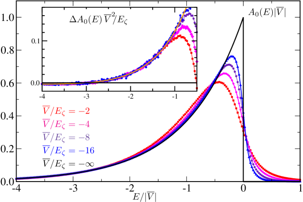
Figure 2: Spectral function $A_{0}(E)$ at zero momentum as function of energy $E$ (in units of rms potential strength $|\overline{V}|$) in a red-detuned laser speckle potential ($\overline{V}<0$) with Gaussian spatial correlation in $d=2$ dimensions. Main plot: The classical limit (thick black line) strictly vanishes above $T_{\boldsymbol{k}}$, here at zero energy. Quantum corrections round this discontinuity. Inset: The semiclassical correction (77) captures the smooth behaviour away from the singularity; the data points for low enough energy collapse onto $(3-|x|)e^{-|x|}/6$, shown as the continous orange curve on top of the data points.

At zero momentum, the quantum correction reads

$$\Delta A_{0}(E)\approx-\frac{dE_{\zeta}}{12\overline{V}^{2}}f^{\prime\prime\prime}(E/\overline{V})$$ (77)

with $f(x)=\Theta(x)xe^{-x}$. Keeping in mind that $\delta(x)\varphi(x)\equiv\delta(x)\varphi(0)$, one finds $f^{\prime\prime\prime}(x)=\delta^{\prime}(x)-2\delta(x)+\Theta(x)(3-x)e^{-x}$ for the leading quantum corrections.

Figure 2 shows numerical data for a red-detuned speckle potential with $\overline{V}<0$ where the successive curves approach the classical distribution, the rising exponential on the negative real axis, with a discontinuity at the origin. The smooth quantum corrections away from the singular point are indeed captured correctly by (77). Close to the origin, however, they are not simply given by the singular terms $\propto[\delta^{\prime}(x)-2\delta(x)]$ of the Wigner-Weyl correction. Here, the quantum corrections are of a different nature. This behaviour is even more pronounced in a blue-detuned speckle potential with $\overline{V}>0$, shown in fig. 3. The quantum corrections close to the absolute lower bound of the classical distribution are highly singular because they must preserve the support of the spectral function on the positive real axis (since both kinetic and potential energy are non-negative, contrary to the red-detuned case where kinetic and potential energy can compensate each other).

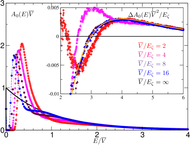
Figure 3: Spectral function $A_{0}(E)$ at zero momentum as function of energy $E$ (in units of rms potential strength $\overline{V}$) in a blue-detuned laser speckle potential ($\overline{V}>0$) with Gaussian spatial correlation in $d=2$ dimensions. Main plot: The classical limit (thick black line) has a strict lower bound at zero energy, which induces large singular quantum corrections. Inset: The semiclassical correction (77) captures the smooth high-energy behaviour. Scales are chosen such that data points progressively collapse onto $(x-3)e^{-x}$, shown as the continuous orange curve on top of the data points.

5.4 Average density of states

The classical average density of states (19) in $d=2$ and for the blue-detuned speckle is

$$\nu^{\text{cl}}(E)=N_{2}\Theta(E)(1-e^{-E/\overline{V}}),\qquad(\overline{V}>0).$$ (78)

There are strictly no states below zero because the potential is bounded from below, and the AVDOS then rises on the scale $\overline{V}$ to its free value $N_{2}$. For the red-detuned speckle, one has

$$\nu^{\text{cl}}(E)=N_{2}\left[\Theta(-E)e^{-E/\overline{V}}+\Theta(E)\right],\qquad(\overline{V}<0).$$ (79)

Here, the rise to the bare DOS above zero energy happens for negative energies. Both these behaviours are qualitatively very similar to the 1d case that has been studied in detail by Falco et al. [13]. Our systematic quantum correction to these limits then is obtained by inserting (76) into (3) and thus reads

$$\Delta\nu(E)\approx-\frac{N_{2}E_{\zeta}}{12|\overline{V}|}f^{\prime\prime}(E/\overline{V}),$$ (80)

with $f(x)=\Theta(x)xe^{-x}$ and thus $f^{\prime\prime}(x)=\delta(x)+\Theta(x)(x-2)e^{-x}$. For the reasons explained in the preceding section, we cannot expect the singular correction around $E=0$ to be accurate. However, at large enough distance from the singular point, the smooth correction is proportional to $(E-2\overline{V})$ and thus predicts an approximate crossing of curves at $E=2\overline{V}$.

6 Summary and outlook

In this paper, quantum corrections to the deep classical limit of matter-wave spectral functions in random potentials have been calculated using the Wigner-Weyl expansion for the smooth contribution of point-like periodic orbits. These corrections are expressed in closed form in terms of the one-point potential distribution and its spatial covariance curvature. A comparison to numerical data for two-dimensional systems reveals that the leading-order Wigner-Weyl corrections apply, as expected, with quantitative agreement to generic Gaussian-distributed potentials. But we also observe that for laser speckle potentials, the smooth corrections only apply in the large-energy sector, where the spectral weight is rather small.

So-called oscillatory contributions from periodic orbits of finite length have been neglected throughout. This approximation can be expected to be valid whenever these orbits depend very sensitively upon the detailed potential configuration for each realisation of disorder. An average over either an energy range or an ensemble of realisations then wipes out these fluctuations. Obviously, this approximation works well with the Gaussian random potential of section 4, where the main spectral weight lies at energies $|E|\lesssim\delta V$ around the mean potential, much above the deep wells. In contrast, for the speckle potential of section 5 quantum corrections beyond the smooth Wigner-Weyl terms are important, because a rather large spectral weight is located close to $E=0$, where the classical distribution is discontinuous, and corrections are of a more singular nature. Indeed, their physical origin then is the zero-point energy shift $\hbar\omega/2$ of locally bound states, where $\omega\propto\sqrt{V^{\prime\prime}_{0}}$ is of the order of the local harmonic oscillator frequency. In principle, such a correction can be described as the result of finite-size periodic orbits, located in the local potential minima. These short trajectories at low energies are all very similar to each other, and their effect can survive the ensemble average. The quantitative treatment of these corrections is beyond the scope of this paper and remains a subject for future research.

Appendix A Numerical methods

In order to test our analytical predictions, we have performed extensive numerical calculations of the spectral function for various types of disorder in $d=2$ dimensions. For the Gaussian-distributed potential discussed in section 4, our data reproduce results available in the literature [1]. The starting point is (2) and the following temporal representation of the $\delta$ function:

$$\delta(E-\hat{H})=\frac{1}{\pi}\mathrm{Im}\frac{1}{E-\hat{H}-\rmi 0}=\frac{1}{\pi}\mathrm{Re}\int_{0}^{\infty}{\rme^{-\rmi\hat{H}t}\ \rme^{\rmi Et}\ \rmd t},$$ (81)

which give

$$A_{{\boldsymbol{k}}}(E)=\frac{1}{\pi}\mathrm{Re}\int_{0}^{\infty}{\overline{\langle{\boldsymbol{k}}|\rme^{-\rmi\hat{H}t}|{\boldsymbol{k}}\rangle}\ \rme^{\rmi Et}\ \rmd t}.$$ (82)

The numerical calculation then amounts to propagating an initial plane wave $|{\boldsymbol{k}}\rangle$ with the disordered Hamiltonian $\hat{H}$ during time $t$ and to computing the overlap of the time evolved state with $\langle{\boldsymbol{k}}|,$ followed by a Fourier transform from time to energy. This step must be repeated for several independent realizations of the disorder in order to perform disorder averaging. In order to obtain small statistical fluctuations even in the tail of the spectral function, a rather large number (more than 120 000) of disorder realizations was used. An alternative numerical method [9] consists in computing eigenstates close to $E$ and determining their momentum representation, followed by an ensemble average. The latter method turns out to consume much more computational resources.

The system is first discretized on a 2D grid of size $L\times L$ with periodic boundary conditions along $x$ and $y$. The spatial discretization step must be much smaller than both the correlation length of the disordered potential and the typical de Broglie wavelength of the propagated state. Typically, a cell of surface $(\pi\zeta)^{2}$ is discretized in 8-20 steps (depending on the disorder strength) along both $x$ and $y$. A spatially correlated complex Gaussian field is generated on the grid in a standard way, by convoluting a spatially uncorrelated complex Gaussian field with a proper cutoff function [36, 10]. The Gaussian correlated potential is obtained by simply taking the real part of the complex field. The speckle potential is obtained by taking the squared modulus of the complex field.

Also, the system size must be chosen much larger than the scattering mean free path at all energies where the spectral function is significant. In practice, a size $L=20\pi\zeta$ was found sufficient.

The CPU-consuming part of our calculation is the temporal propagation of the initial state $|{\boldsymbol{k}}\rangle$ with the disordered Hamiltonian $\hat{H}.$ The time propagation itself uses an iterative method based on the expansion of the evolution operator in combinations of Chebyshev polynomials of the Hamiltonian [37, 38]. This procedure is repeated for many disorder realizations, which finally gives access to the spectral function. Since the spectral function is a smooth function of energy, its Fourier transform decays relatively fast at long times. This makes it possible to numerically propagate the initial state $|{\boldsymbol{k}}\rangle$ only over a restricted time interval, which reduces the computing time substantially.

References

References

- [1] R. Zimmermann and C. Schindler, Phys. Rev. B 80, 144202 (2009).
- [2] G. Modugno, Rep. Progr. Phys. 73, 102401 (2010).
- [3] L. Sanchez-Palencia and M. Lewenstein, Nat. Phys. 6, 87 (2010).
- [4] B. Shapiro, J. Phys. A: Math. Theor. 45, 143001 (2012).
- [5] S. S. Kondov, W. R. McGehee, J. J. Zirbel, and B. DeMarco, Science 334, 66 (2011).
- [6] W. R. McGehee, S. S. Kondov, W. Xu, J. J. Zirbel, and B. DeMarco, Phys. Rev. Lett. 111, 145303 (2013).
- [7] C. A. Müller and B. Shapiro, Phys. Rev. Lett. 113, 099601 (2014).
- [8] W. R. McGehee, S. S. Kondov, W. Xu, J. J. Zirbel, and B. DeMarco, Phys. Rev. Lett. 113, 099602 (2014).
- [9] G. Semeghini et al., Measurement of the mobility edge for 3D Anderson localization, 2014, arXiv:1404.3528.
- [10] D. Delande and G. Orso, Phys. Rev. Lett. 113, 060601 (2014).
- [11] R. Kuhn, O. Sigwarth, C. Miniatura, D. Delande, and C. A. Müller, New J. Phys. 9, 161 (2007).
- [12] P. Lugan et al., Phys. Rev. A 80, 023605 (2009), arXiv:0902.0107.
- [13] G. M. Falco, A. A. Fedorenko, J. Giacomelli, and M. Modugno, Phys. Rev. A 82, 053405 (2010).
- [14] H. Bruus and K. Flensberg, Many-Body Quantum Theory in Condensed Matter Physics (Oxford Univ. Press, 2004).
- [15] R. C. Kuhn, C. Miniatura, D. Delande, O. Sigwarth, and C. A. Müller, Phys. Rev. Lett. 95, 250403 (2005).
- [16] A. Yedjour and B. A. Tiggelen, Eur. Phys. J. D 59, 249 (2010).
- [17] M. Piraud, L. Pezzé, and L. Sanchez-Palencia, New J. Phys. 15, 075007 (2013).
- [18] E. P. Wigner, Ann. Mathem. 62, pp. 548 (1955).
- [19] T. A. Brody et al., Rev. Mod. Phys. 53, 385 (1981).
- [20] E. O. Kane, Phys. Rev. 131, 79 (1963).
- [21] L. Pezzé et al., New J. Phys. 13, 095015 (2011).
- [22] P. Gaspard, -expansion for quantum trace formula, in Quantum Chaos: Between Order and Disorder, edited by G. Casati and B. Chirikov, pp. 385–404, Cambridge Univ. Press, 1995.
- [23] K. Richter, Semiclassical Theory of Mesoscopic Quantum Systems (Springer Berlin Heidelberg, 2000).
- [24] E. Wigner, Phys. Rev. 40, 749 (1932).
- [25] H. J. Groenewold, Physica 12, 405 (1946).
- [26] J. E. Moyal, Math. Proc. Camb. Phil. Soc. 45, 99 (1949).
- [27] K. Imre, E. Özizmir, M. Rosenbaum, and P. F. Zweifel, J. Math. Phys. 8, 1097 (1967).
- [28] M. Hillary, R. F. O’Connell, M. O. Scully, and E. P. Wigner, Phys. Rep. 106, 121 (1984).
- [29] N. L. Balazs and B. K. Jennings, Phys. Rep. 104, 347 (1984).
- [30] B.-G. Englert, J. Phys. A: Math. Gen. 22, 625 (1989).
- [31] C. Gneiting, T. Fischer, and K. Hornberger, Phys. Rev. A 88, 062117 (2013).
- [32] T. Fischer, C. Gneiting, and K. Hornberger, New J. Phys. 15, 063004 (2013).
- [33] C. K. Zachos, D. B. Fairlie, and T. L. Curtright, Quantum Mechanics in Phase Space (World Scientific, 2005).
- [34] B. Grammaticos and A. Voros, Ann. Phys. 123, 359 (1979).
- [35] M. Cinal and B.-G. Englert, Phys. Rev. A 48, 1893 (1993).
- [36] R. Kuhn, Coherent Transport of Matter Waves in Disordered Optical Potentials, PhD thesis, Universität Bayreuth, 2007.
- [37] S. Roche and D. Mayou, Phys. Rev. Lett. 79, 2518 (1997).
- [38] H. Fehske et al., Phys. Lett. A 373, 2182 (2009).