Infinite Object Coating in the Amoebot Model

The term programmable matter refers to matter which has the ability to change its physical properties (shape, density, moduli, conductivity, optical properties, etc.) in a programmable fashion, based upon user input or autonomous sensing. This has many applications like smart materials, autonomous monitoring and repair, and minimal invasive surgery. While programmable matter might have been considered pure science fiction more than two decades ago, in recent years a large amount of research has been conducted in this field. Often programmable matter is envisioned as a very large number of small locally interacting computational particles. We propose the Amoebot model, a new model which builds upon this vision of programmable matter. Inspired by the behavior of amoeba, the Amoebot model offers a versatile framework to model self-organizing particles and facilitates rigorous algorithmic research in the area of programmable matter. We present an algorithm for the problem of coating an infinite object under this model, and prove the correctness of the algorithm and that it is work-optimal.

1 Introduction

Recent advances in microfabrication and cellular engineering foreshadow that in the next few decades it might be possible to assemble myriads of simple information processing units at almost no cost. Microelectronic mechanical components have become so inexpensive to manufacture that one can anticipate integrating logic circuits, microsensors, and communications devices onto nano-computational components. Imagine coating bridges and buildings with smart paint that senses and reports on traffic and wind loads and monitors structural integrity. A smart-paint coating on a wall could sense vibrations, monitor the premises for intruders, and cancel noise. There has also been amazing progress in understanding the biochemical mechanisms in individual cells such as the mechanisms behind cell signaling and cell movement [3]. Recently, it has been demonstrated that, in principle, biological cells can be turned into finite automata [8] or even pushdown automata [35], so one can imagine that some day one can tailor-make biological cells to function as sensors and actuators, as programmable delivery devices, and as chemical factories for the assembly of nano-scale structures.

One can envision producing vast quantities of individual microscopic computational particles—whether microfabricated particles or engineered cells—to form programmable matter, as coined by Toffoli and Margolous [44]. These particles are possibly faulty, sensitive to the environment, and may produce various types of local actions that range from changing their internal state to communicating with other particles, sensing the environment, moving to a different location, changing shape or color, or even replicating. Those individual local actions may then be used to change the physical properties, color, and shape of the matter at a global scale.

We propose Amoebot, a new amoeba-inspired model for programmable matter. In our model, the programmable matter consists of particles that can bond to neighboring particles and use these bonds to form connected structures. Particles only have local information and have modest computational power: Each particle has only a constant-size memory and behaves similarly to a finite state machine. The particles act asynchronously and they achieve locomotion by expanding and contracting, which resembles the behavior of amoeba [3].

1.1 Our Contributions

Our proposed Amoebot model, presented in Section 3, offers a versatile framework to model self-organizing particles and facilitates rigorous algorithmic research in the area of programmable matter. In addition, we present an algorithm for the problem of coating an infinite object under this model in Section 5.2, and prove the correctness of the algorithm (Theorem 1) and that the algorithm is work-optimal (Theorem 2).

2 Related Work

While programmable matter may have seemed like science fiction more than two decades ago, we have seen many advances in this field recently. One can distinguish between active and passive systems. In passive systems the particles either do not have any intelligence at all (but just move and bond based on their structural properties or due to chemical interactions with the environment), or they have limited computational capabilities but cannot control their movements. Examples of research on passive systems are DNA computing [1, 10, 14, 20, 38, 48], tile self-assembly systems in general [41, 42], population protocols [4], and slime molds [11, 36, 46]. We will not describe these models in detail as they are only of little relevance for our approach. On the other hand in active systems, there are computational particles that can control the way they act and move in order to solve a specific task. Self-organizing networks, robotic swarms, and modular robotic systems are some examples of active systems.

Self-organizing networks have been studied in many different contexts. Networks that evolve out of local, self-organizing behavior have been heavily studied in the context of complex networks such as small-world networks [6, 33, 47]. However, whereas a common approach for the complex networks field is to study the global effect of given local interaction rules, we aim at developing local interaction rules in order to obtain a desired global effect.

In the area of swarm robotics it is usually assumed that there is a collection of autonomous robots that have limited sensing, often including vision, and communication ranges, and that can freely move in a given area. They follow a variety of goals, as for example graph exploration (e.g., [27]), gathering problems (e.g., [2, 16]) , and shape formation problem (e.g., [28]). Surveys of recent results in swarm robotics can be found in [32, 37]; other samples of representative work can be found in e.g.,  [25, 7, 18, 19, 17, 31, 30, 43, 26, 39, 34, 5, 40]. Besides work on how to set up robot swarms in order to solve certain tasks, a significant amount of work has also been invested in order to understand the global effects of local behavior in natural swarms like social insects, birds, or fish (see e.g., [13, 9]). While the analytical techniques developed in the area of swarm robotics and natural swarms are of some relevance for this work, the underlying model differs significantly as we do not allow free movement of particles.

While swarm robotics focuses on inter-robotic aspects in order to perform certain tasks, the field of modular self-reconfigurable robotic systems focuses on intra-robotic aspects such as the design, fabrication, motion planning, and control of autonomous kinematic machines with variable morphology (see e.g., [29, 50]). Metamorphic robots form a subclass of self-reconfigurable robots that shares the characteristics of our model that all particles are identical and that they fill space without gaps [15]. The hardware development in the field of self-reconfigurable robotics has been complemented by a number of algorithmic advances (e.g., [12, 45]), but so far mechanisms that scale to hundreds or thousands of individual units are still under investigation, and no rigorous theoretical foundation is available yet.

As in our model, the work in [24] also assumes that each system particle is a finite state machine with constant-size memory operating in an asynchronous distributed fashion. However, the work in [24] assumes a static network topology and the problems considered only address what can be computed in an asynchronous network of randomized constant-size memory finite state machines, and not how desired topology/shape can be achieved in systems where finite state machine particles can move (in addition to computing).

The nubot model [49], by Woods et al., was developped independently to our model (our model was originally presented at the First Workshop on Biological Distributed Algorithms (BDA), October 2013 [22, 21]), and aims at providing the theoretical framework that would allow for a more rigorous algorithmic study of biomolecular-inspired systems, more specifically of self-assembly systems with active molecular components. While our model shares many similarities with the nubot model at a high level, many of the assumptions underlying the nubot model are different from ours: For example, in the nubot model, particles are allowed to replicate at will and are allowed to drag many other particles as they move in space (which is pertinent in many molecular level systems, but which would not be feasible in systems with very large numbers of nano-robots with weak bond structures); also the number of states (and hence also the memory size) that a particle can be in is proportional to $\log n$—where $n$ relates to the number of particles in the final desired configuration the system should assume—whereas in our model the number of possible states is assumed to be constant.

3 Model

Consider the equilateral triangular graph $G_{eqt}$, see Figure1.

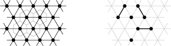
Figure 1: The left half of the figure depicts a section of the infinite equilateral triangular graph $G_{eqt}$. Nodes are shown as black circles. For four of the nodes the dual faces in the hexagonal tiling of the Euclidean plane are shown in gray. The right half shows five particles on the graph. When depicting particles we draw the graph as a gray mesh without nodes. A particle occupying a single node is depicted as a black circle, and a particle occupying two nodes is depicted as two black circles connected by an edge.

A particle occupies either a single node or a pair of adjacent nodes in $G_{eqt}$, and every node can be occupied by at most one particle. Two particles occupying adjacent nodes are defined to be connected and we refer to such particles as neighbors. The graph $G_{eqt}$ is the dual graph of the hexagonal tiling of the Euclidean plane as indicated in Figure 1. So geometrically the space occupied by a particle is bound by either one face or two adjacent faces in this tiling of the plane.

Every particle has a state from a finite set $Q$. Connected particles can communicate via the edges connecting them in the following way. A particle $p$ holds a flag from a finite alphabet $\Sigma$ for each edge that is incident to $p$ (i.e., all edges incident to a node occupied by $p$ except the edge between the occupied nodes if $p$ occupies two nodes). A particle occupying the node on the other side of such an edge can read this flag. This communication process can be used in both directions over an edge. In order to allow a particle $p$ to address the edges incident to it, the edges are labeled from the local perspective of $p$. This labeling starts with $0$ at an edge leading to a node that is only adjacent to one of the nodes occupied by $p$ and increases counter-clockwise around the particle.

Particles move through expansion and contraction: If a particle occupies one node, it can expand into an unoccupied adjacent node to occupy two nodes. If a particle occupies two nodes, it can contract out of one of these nodes to occupy only a single node. (Those two actions can be naturally physically realized on the dual hexagonal tiling of the Euclidean plane.) Accordingly, we call a particle occupying a single node contracted and a particle occupying two nodes expanded. Note that we can identify six directions in our graph corresponding to the directions of the six edges incident to a node. The direction of the edge labeled $0$ is defined to remain constant throughout all movement. We call this direction the orientation of a particle. Figure 2 shows an example of the movement of a particle.

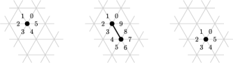
Figure 2: The three parts of the figure show a moving particle together with the labels seen by the particle. On the left, the particle occupies only a single node. The particle then expands in the direction of the edge labeled $4$ resulting in the particle occupying two nodes as depicted in the middle. Since the expansion changes the number of edges incident to the particle, the edges have to be relabeled. The direction of the edge labeled $0$ remains constant. Next the particle contracts out of one of the nodes it currently occupies towards the direction of the edge labeled $6$ resulting in the particle occupying only a single node as depicted on the right. Again, the edges incident to the particle are relabeled.

Besides executing expansions and contractions in isolation, we allow pairs of connected particles to combine these primitives to perform a coordinated movement: One particle can contract out of a certain node at the same time as another particle expands into that node. We call this movement a handover, see Figure 3.

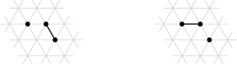
Figure 3: Two particles performing a handover.

The particles involved in a handover are defined to remain connected during its execution.

Computationally, particles resemble finite state machines. A particle acts according to a transition function

$$\delta:\;Q\times\Sigma^{10}\;\to\;\mathcal{P}(Q\times\Sigma^{10}\times M).$$

For a particle $p$ the function takes the current state of $p$ and the flags $p$ can read via its incident edges as arguments. Here, the $i$-th coordinate of the tuple $\Sigma^{10}$ represents the flag read via the edge labeled $i$ when numbering the coordinates of the tuple starting at $0$. If for a label $i$ there is no edge with that label or if the respective edge leads to a node that is not occupied, the coordinate of the tuple is defined to be $\varepsilon$. The value $\varepsilon\in\Sigma$ is reserved for this purpose and cannot be set as a flag by a particle. The transition function maps to a set of turns. A turn is a tuple specifying a state to assume, flags to set, and a movement to execute. The set of movements is defined as

$$M=\{\text{idle}\}\;\cup\;\{\text{expand}_{i}\mid i\in[0,9]\}\;\cup\;\{\text{contract}_{i}\mid i\in[0,9]\}\;\cup\;\{\text{handoverContract}_{i}\mid i\in[0,9]\}.$$

The movement idle means that $p$ does not move, and expand_i and contract_i are defined as mentioned above. The index $i$ specifies the edge that defines the direction along which the movement should take place, as shown in the example in Figure 2. Note that there are only two possible directions for a contract operation. The movement handoverContract_i specifies a contraction that can only be executed as part of a handover. In summary, a transition function specifies a set of turns a particle would like to perform based on the locally available information.

A system of particles progresses by executing atomic actions. An action is either the execution of an isolated turn for a single particle or the execution of a turn for each of two particles resulting in a handover between those particles. Note that if a movement is not executable, the respective action is not enabled: For example, a particle occupying two nodes cannot expand although it might specify this movement in a turn. As another example, a particle cannot expand into an occupied node except as part of a handover. Finally, an action consisting of an isolated turn involving the movement handoverContract_i is never enabled as this movement can only be performed as part of a handover. The transition function is applied for each particle to determine the set of enabled actions in the system. From this set, a single action is arbitrarily chosen and executed. The process of evaluating the transition function and executing an action continues as long as there is an enabled action.

Two actions are said to be independent if they do not involve nodes that are neighbors in $G_{eqt}$. Each particle can locally ensure that at most one action in its neighborhood is executed at any point in time. Hence, all of our results also hold if a set of mutually independent actions was chosen to be concurrently executed at any point in time.

4 Morphing Problems

In general, we define a morphing problem as being a problem in which a system of particles has to morph into a shape with specific characteristics (by changing the positioning of the particles in $G_{eqt}$) while sustaining connectivity. Examples of morphing problems are the formation of geometric shapes and coating objects (i.e., surrounding a given set of nodes). Before we can formally define morphing problems, we need some definitions.

We define the configuration of a particle as the tuple of its state, its flags, the set of nodes it occupies, and its orientation. A system of particles progresses by performing atomic actions, each of which affects the configuration of one or two particles. Therefore, a system progresses through a sequence of configurations where a configuration of a system is the set of configurations of all its particles. We define the connectivity graph $G(c)$ of a configuration $c$ as the subgraph of $G_{eqt}$ induced by the occupied nodes in $c$.

We can formally define a morphing problem as a tuple $M=(I,G)$ where $I$ and $G$ are sets of connected configurations. We say $I$ is the set of initial configurations and $G$ is the set of goal configurations. An algorithm $A$, formally defined by a transition function $\delta$, solves $M$ if three conditions hold: Consider the execution of $A$ on a system in an arbitrary configuration from $I$. First, the system stays connected throughout the execution of $A$. Second, the execution eventually reaches a configuration in which the transition function of each particle maps to the empty set (we say $A$ terminates). Third, when the execution terminates, the reached configuration is from $G$.

5 Infinite Object Coating

As a subclass of the class of morphing problems, one can consider coating problems in which an object is to be coated (i.e., surrounded or engulfed) by the particles of a system as uniformly as possible. We investigate the Infinite Object Coating problem where the object has an infinite surface and, accordingly, a uniform coating is accomplished when all the particles of a system are directly connected to the object.

5.1 Problem Definition

In the Infinite Object Coating problem, an object can be represented by a set of contracted particles occupying nodes in $G_{eqt}$. These particles are in a special object state, and we refer to these particles as object particles. A transition function must map to the empty set for an object particle, and no particle can switch into the object state. We denote the number of non-object particles in a system by $n$. In the reminder of this paper, unless otherwise stated, when we refer to a particle, we mean a non-object particle. We say a particle lies on the surface of the object if it is connected to an object particle. Consider a connected induced subgraph $C$ of $G_{eqt}$. The subgraph $C$ is called compact if $G_{eqt}-C$ is $2$-connected. An object that induces a compact subgraph in $G_{eqt}$ is a valid object. Intuitively, this definition means that a valid object cannot have tunnels of width one, see Figure 4. Disallowing these tunnels allows particles to move along the object in single file (as will be described in Section 5.2.1) without blocking each other and therefore improves the clarity of presentation by avoiding boundary cases.

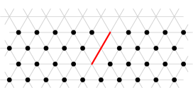
Figure 4: An example of an invalid object. The object occupies a half-plane except for the nodes marked by the solid line. These nodes form a tunnel of width one in the object since removing the topmost of these nodes from $G_{eqt}-C$ disconnects the two remaining nodes in that graph.

As presented in Section 4, a morphing problem is defined as a tuple $(I,G)$ where $I$ is a set of initial configurations and $G$ is a set of goal configurations. For the Infinite Object Coating problem, $I$ is the set of all connected configurations consisting of a valid object together with a finite set of contracted particles. Every particle stores a phase as part of its state and in an initial configuration every particle is in an inactive phase; we will elaborate on phases in Section 5.2.2. Similarly, the set $G$ is the set of all configurations consisting of a valid object together with a finite set of contracted particles that all lie on the surface of the object.

The general Amoebot model as described in Section 3 can take various specific forms depending on how systems of particles are initialized, what information particles keep track of in their state, and what information they share over their edges. In the Infinite Object Coating problem, we do not make any assumption about the orientation of the particles. Therefore, we work in a no-compass variant of the model. While particles do not share a common sense of direction, they are able to keep track of directions by storing edge labels in their state and updating these labels upon movement. The updates can be encoded in the transition function. We assume that a particle keeps track of whether it is contracted or expanded; the particle also keeps track of which edge labels are incident to the occupied node that is an endpoint of the edge labeled $0$. Additionally, we assume that for an edge with label $i$ the corresponding flag always includes the index $i$, the information whether the edge is incident to the occupied node that is an endpoint of the edge labeled $0$, and whether the particle is contracted or expanded. Using this information, a particle that reads a flag can compare its orientation to the orientation of the particle that set the flag and therefore particles can exchange information about directions. Lastly, we assume that a particle keeps track of what edge labels specify valid contraction indices.

For the sake of generality, the Amoebot model does not enforce any fairness condition on the execution of actions. However, for the Infinite Object Coating problem we make the following assumption: Any set of of consecutive configurations in which a particle $p$ could be affected by an enabled action, but is not, is finite.

5.2 Algorithm

Our algorithm for the Infinite Object Coating problem is a combination of three algorithmic primitives. First, particles lying on the surface of the object lead the way by moving in a common direction along the surface. Second, the remaining particles follow behind the leading particles resulting in the system flattening out towards the direction of movement. Third, particles on the surface check whether there are particles not lying on the surface and use this information to eventually achieve termination. We present each of these primitives in detail in the following sections.

5.2.1 Moving Along a Surface

Our first algorithmic primitive solves a simple problem: We want all particles on the surface to move along the surface in a common direction. However, before we can present our algorithm for this problem, we need some definitions. For an expanded particle, we denote the node the particle last expanded into as the head of the particle and call the other occupied node its tail. For a contracted particle, we define the single occupied node to be both the head and the tail. The set of labels associated to the edges incident to the head can be encoded as part of the state, and this information can be set upon expansion as part of the transition function. Therefore, a particle can always distinguish the labels of edges incident to its head (head labels) from the labels of edges incident to its tail (tail labels). Accordingly, we call edges that are labeled with a head label head edges and the remaining edges tail edges. Combined with the information about valid contraction indices described in Section 5.1, a particle can deliberately contract out of its tail or its head. In our algorithm, particles are only allowed to contract out of their tails so that the fact that a particle contracts uniquely defines the contraction direction. Note that with this convention, the head of a particle still is occupied by that particle after a contraction.

A particle on the surface can move along the surface in two directions. However, we want all particles on the surface to move in a common direction. The simple procedure given in Algorithm 1, which is very similar to the moving algorithm presented by Drees et al. [23], can be used to achieve this goal:

let $k$ be the size of the neighborhood of the particle (i.e., $k=6$ or $k=10$)

let $i$ be the label of an edge connected to the object

while edge $i$ is connected to the object do

     $i\;\leftarrow\;(i-1)\mod k$

return $i$

Algorithm 1 Movement along a Surface

A contracted particle uses the procedure to compute the direction of an expansion, and an expanded particle simply contracts according to above definitions. The correctness of this approach is based on two facts. First, all particles share a common sense of rotation (i.e., the edge labels always increase counter-clockwise around a particle). Second, according to our definition of a valid object, an object must occupy a single consecutive sequence of nodes around a particle from the local perspective of that particle and not all nodes around a particle belong to the object.

5.2.2 Spanning Forest Algorithm

As the name suggests, the spanning forest algorithm aims to organize the particles in a system as a spanning forest where the particles that represent the roots of the trees in the forest are considered leaders whom the remaining particles follow. Therefore, the movement of the system is dominated by the movement of the leaders. Every particle that is connected to the surface becomes a leader, and leaders move along the surface as described in the previous section. Algorithm 2 provides a detailed description of this approach.

A particle is in one of three phases inactive, follow, and lead. Initially, all particles are assumed to be in phase inactive. The phase of a particle is encoded as part of its state, and a particle indicates its phase as part of all its flags. We call a particle in phase follow a follower and a particle in phase lead a leader. A follower stores a head label $d$ in its state and includes a follow indicator in the flag for the edge with label $d$. Depending on its phase, a particle $p$ behaves as described below. The transition function maps either to a set containing a single turn or to the empty set. The specified conditions are to be checked in the given order. If a condition holds, the transition function maps to the set containing only the respective turn. If none of the conditions holds, the transition function maps to the empty set. inactive: If $p$ is connected to the surface, it becomes a leader and executes the idle movement. If an adjacent node is occupied by a leader or a follower, $p$ sets $d$ to point towards that node and becomes a follower. follow: If $p$ is contracted and connected to the surface, it becomes a leader and executes the idle movement. If $p$ is contracted and there is an expanded particle $p^{\prime}$ occupying the node reached via the edge labeled $d$, $p$ expands in direction $d$ as an attempt to a handover and sets $d$ to correspond to the contraction direction of $p^{\prime}$. If $p$ is expanded and a follow indicator is read from a contracted neighbor over a tail edge, $p$ executes a handover contraction and changes $d$ to keep the direction constant. If $p$ is expanded, no follow indicator is read over a tail edge, and $p$ has no inactive neighbor, $p$ contracts and changes $d$ to keep the direction constant. lead: If $p$ is contracted, it expands in the direction computed by Algorithm 1. If $p$ is expanded and a follow indicator is read from a contracted neighbor over a tail edge, $p$ executes a handover contraction. If $p$ is expanded, no follow indicator is read over a tail edge, and there is no inactive neighbor, $p$ contracts.

Algorithm 2 Spanning Forest Algorithm

In contrast to particles in phase inactive, we say followers and leaders are active. As specified in Algorithm 2, the value $d$ is only defined for followers. We denote the node in $G_{eqt}$ reached from a follower $p$ via the edge labeled $d$ as $u(p)$. The following lemmas demonstrate some properties that hold during the execution of the spanning forest algorithm and will be used in Section 5.3 to analyze our complete algorithm.

Lemma 1

For a follower $p$ the node $u(p)$ is occupied by an active particle.

Proof.  Consider a follower $p$ in any configuration during the execution of Algorithm 2. Note that $p$ can only get into phase follow from phase idle, and once it leaves the follow phase it will not switch to that phase again. Consider the first configuration $c_{1}$ in which $p$ is a follower. In the configuration $c_{0}$ immediately before $c_{1}$, $p$ must be inactive and it becomes a follower because of an active particle $p^{\prime}$ occupying $u(p)$ in $c_{0}$. The particle $p^{\prime}$ still occupies $u(p)$ in $c_{1}$. Now assume that $u(p)$ is occupied by an active particle $p^{\prime}$ in a configuration $c_{i}$, and that $p$ is still a follower in the next configuration $c_{i+1}$ that results from executing an action $a$. If $a$ affects $p$ and $p^{\prime}$, the action must be a handover in which $p$ updates its value $d$ such that $u(p)$ changes but $p^{\prime}$ again occupies $u(p)$ in $c_{i+1}$. If $a$ affects $p$ but not $p^{\prime}$, it must be a contraction in which $u(p)$ does not change and is still occupied by $p^{\prime}$. If $a$ affects $p^{\prime}$ but not $p$, there are multiple possibilities. The particle $p^{\prime}$ might switch from phase follow to phase lead or it might expand, neither of which violate the lemma. Furthermore, $p^{\prime}$ might contract. If $u(p)$ is the head of $p^{\prime}$, $p^{\prime}$ still occupies $u(p)$ in $c_{i+1}$. Otherwise, $p^{\prime}$ reads a follow indicator from $p$ over a tail edge in $c_{i}$ and therefore the contraction must be part of a handover. As $p$ is not involved in the action, the handover must be between $p^{\prime}$ and a third active particle $p^{\prime\prime}$. It is easy to see that after such a handover $u(p)$ is occupied by either $p^{\prime}$ or $p^{\prime\prime}$. Finally, if $a$ affects neither $p$ nor $p^{\prime}$, $u(p)$ will still be occupied by $p^{\prime}$ in $c_{i+1}$. $\sqcap$$\sqcup$

Based on Lemma 1, we define a successor relation on the active particles in a configuration $c$. Let $p$ be a follower. We say $p^{\prime}$ is the successor of $p$ if $p^{\prime}$ occupies $u(p)$. Analogously, we say $p$ is a predecessor of $p^{\prime}$. Furthermore, we define a directed graph $A(c)$ for a configuration $c$ as follows. $A(c)$ contains the same nodes as $G(c)$. For every expanded particle $p$ in $c$, $A(c)$ contains a directed edge from the tail to the head of $p$, and for every follower $p^{\prime}$ in $c$, $A(c)$ contains a directed edge from the head of $p^{\prime}$ to $u(p^{\prime})$.

Lemma 2

The graph $A(c)$ is a forest, and if there is at least one active particle, every connected component of inactive particles contains a particle that is connected to an active particle.

Proof.  In an initial configuration $c_{0}$, all particles are inactive and therefore the lemma holds trivially. Now assume that the lemma holds for a configuration $c_{i}$. We will show that it also holds for the next configuration $c_{i+1}$ that results from executing an action $a$. If $a$ affects an inactive particle $p$, this particle either becomes a follower or a leader. In the former case $p$ joins an existing tree, and in the latter case $p$ forms a new tree in $A(c_{i+1})$. In either case, $A(c_{i+1})$ is a forest and the connected component of inactive particles that $p$ belongs to in $c_{i}$ is either non-existent or connected to $p$ in $c_{i+1}$. If $a$ affects only a single particle $p$ that is in phase follow, this particle can contract or become a leader. In the former case, $p$ has no predecessor $p^{\prime}$ such that $u(p^{\prime})$ is the tail of $p$ and also $p$ has no idle neighbors. Therefore, the contraction of $p$ does not disconnect any follower or inactive particle and, accordingly, does not violate the lemma. In the latter case, $p$ becomes a root of a tree which also does not violates the lemma. If $a$ involves only a single particle $p$ that is in phase lead, $p$ can expand or contract. An expansion trivially cannot violate the lemma and the argument for the contraction is the same as for the contraction of a follower above. Finally, if $a$ involves two active particles in $c_{i}$, these particles perform a handover. While such a handover can change the successor relation among the nodes, it cannot violate the lemma. $\sqcap$$\sqcup$

The following lemma shows that the spanning forest algorithm achieves progress in that as long as the leaders keep moving, the remaining particles will eventually follow them.

Lemma 3

An expanded particle eventually contracts.

Proof.  Consider an expanded particle $p$ in a configuration $c$. Note that $p$ must be active. If there is an enabled action that includes the contraction of $p$, that action will remain enabled until $p$ contracts and therefore $p$ will contract eventually according to the fairness assumption we made in Section 5.1. So assume that there is no enabled action that includes the contraction of $p$. According to the behavior of inactive particles, at some point in time all particles in the system will be active. If the contraction of $p$ becomes part of an enabled action before this happens, $p$ will eventually contract. So assume that all particles are active but still $p$ cannot contract. If $p$ has no predecessors, the isolated contraction of $p$ is an enabled action which contradicts our assumption. Therefore, $p$ must have predecessors. Furthermore, $p$ must read at least one follow indicator over a tail edge and all predecessors from which it reads a follow indicator must be expanded as otherwise $p$ could again contract as part of a handover. Let $p^{\prime}$ be one of the predecessors of $p$. If $p^{\prime}$ would contract, a handover between $p^{\prime}$ and $p$ would become an enabled action. We can apply the complete argument presented in this proof so far to $p^{\prime}$ and so on backwards along a branch in a tree in $A(c)$ until we reach a particle that can contract. We will reach such a particle by Lemma 2. Therefore, we found a sequence of expanded particles that starts with $p^{\prime}$ and ends with a particle that eventually contracts. The contraction of that last particle will allow the particle before it in the sequence to contract and so on. Finally, the contraction of $p$ will become part of an enabled action and therefore $p$ will eventually contract. $\sqcap$$\sqcup$

In the above lemmas, the direction of expansion of leaders is not used. Furthermore, the fact that only particles on the surface become leaders is not used. Therefore, the algorithm works independently of the selection of leaders and their expansion direction. This makes the spanning forest algorithm a reusable algorithmic primitive.

5.2.3 Complaining Algorithm

The algorithm so far achieves that the particles spread out towards one direction on the surface, which will be shown formally in Section 5.3. However, the particles keep moving indefinitely even when all particles lie on the surface. Since we require termination from an algorithm to solve the Infinite Object Coating problem, we need another algorithmic primitive that ensures that once all particles are on the surface, they eventually stop moving. To achieve this, we use the idea of complaining, see Algorithm 3. The algorithm extends Algorithm 2 by changing the set of turns for leaders. The conditions in Algorithm 3 ought to be checked before the conditions given in Algorithm 2.

Consider a leader particle $p$ and let $s$ be the direction returned by Algorithm 1, i.e., the direction that leaders use to travel along the surface. Leaders can include a complaint indicator in a flag. If $p$ is contracted and cannot expand or perform a handover and sees a follow indicator or complaint indicator, it sends a complaint indicator in direction $s$ and performs the idle movement. If $p$ is contracted and does not see a complaint indicator, it does not perform any action. Otherwise $p$ behaves according to Algorithm 2.

Algorithm 3 Complaining Algorithm

Note that a complaint indicator will be consumed by a leader $p$ if it expands, contracts, or performs a handover. That is, as long as all particles which forwarded the indicator have not moved up to $p$, $p$ will not see a complaint indicator. Furthermore, consider a follower $q$ that reached the surface, but is not a leader yet. If $q$ reads a complaint indicator, it will not forward the indicator directly, but as soon as it turns into a leader. Moreover, if all particles are leaders, then no leader sees a follow indicator. We extend the notion of $u(p)$ from Section 5.2.2 to leaders. The node $u(p)$ for a leader $p$ is the node in the direction returned by Algorithm 1. Hence, the notion of successors (i.e., $p^{\prime}$ is a successor of $p$ in some configuration $c$ if $p^{\prime}$ occupies $u(p)$) is now also applicable for leaders. If $u(p)$ is unoccupied, $p$ has no successor. The descendants of a particle $p$ are all nodes reachable by the successor relation (i.e., the successor of, the successor of the successor, and so on). For each particle $p$ we denote the descendant that has no successor with $a(p)$. For the next lemma consider a system that behaves according to Algorithm 2 and Algorithm 3.

Lemma 4

As long as a follower particle $p$ exists, a descendant will eventually expand, and if all particles are leaders the transition function of every leader eventually maps to the empty set.

Proof.  For the first statement assume that even though the particle $p$ exists, no descendant expands. Following our assumption none of the descendants can expand, therefore they all have to be contracted, because an expanded descendant would allow for a handover which involves an expansion. Therefore, a complaint indicator is created by a leader particle that is a descendant of $p$ and sees a follow indicator. This indicator is forwarded among the descendants along the surface until $a(p)$ sees it. Particle $a(p)$ can always expand, which contradicts the assumption.

To prove the second statement, we look at the case in which all particles are leaders. We already mentioned that no more follow indicators exist. Therefore, it is easy to see that all complaint indicators eventually vanish. Accordingly, the transition function of all particles without a neighbor in direction $s$ maps to the empty set. As a result, the transition function of leaders that are neighbors to leaders without a neighbor in direction $s$ will eventually map to the empty set. This process continues until the transition function of every particle maps to the empty set. $\sqcap$$\sqcup$

5.3 Analysis

Now, we can show that our algorithm as developed in the previous three sections solves the Infinite Object Coating problem.

Theorem 1

Our algorithm solves the Infinite Object Coating problem.

Proof.  First, we have to show that the algorithm maintains connectivity. So consider a system of particles in a configuration during the execution of our algorithm. The object is by definition connected. A leader always lies on the surface of the object according to Algorithm 2. A follower is always part of a tree in the spanning forest as shown in Lemma 2. As every tree forms a connected component and is rooted in a leader, the set of object particles and active particles forms a connected component. Finally, an inactive particle is always part of a connected component of inactive particles that includes a particle that is connected to an active particle, again by Lemma 2. Therefore, all particles in the system form a single connected component.

Next, we have to show that the algorithm terminates and that when it does, the system is in a goal configuration. A common property of all goal configurations is that all particles lie on the surface. In our algorithm, every particle $p$ eventually activates. If $p$ initially lies on the surface, it becomes a leader and remains on the surface. If $p$ initially does not lie on the surface, it becomes a follower. Let $c$ be the first configuration in which $p$ is a follower. Consider the directed path in $A(c)$ from the head of $p$ to the first node on the surface. There always is such a path since every follower belongs to a tree in $A(c)$ by Lemma 2, every such tree is rooted in a leader, and a leader only occupies nodes on the surface. Let $P=(u_{0},u_{1},\ldots,u_{k})$ be that path where $u_{0}$ is the head of $p$ and $u_{k}$ lies on the surface. According to Algorithm 2, $p$ attempts to follow $P$ by sequentially expanding into the nodes $u_{1},\ldots,u_{k}$. By Lemma 4, the algorithm does not terminate before $p$ reaches the surface, and according to Lemma 3, $p$ can actually execute all movements required to follow $P$. Therefore, $p$ eventually lies on the surface, becomes a leader, and remains on the surface. According to Lemma 4 this means that for all particles the transition function eventually maps to the empty set which implies termination. $\sqcap$$\sqcup$

Finally, we would like to measure how well our algorithm performs in terms of energy consumption. For this, we consider the number of movements executed in a system until termination and call this measure work. When we refer to movement in the context of work, we only mean expansions and contraction but not idle movements. We count a handover as two movements. We ignore any computation a particle performs since in a physical realization the energy consumption of computation is most likely negligible compared to the energy consumption of movement.

Lemma 5

The worst-case work required by any algorithm to solve the Infinite Object Coating problem is $\Omega(n^{2})$.

Proof.  Consider the configuration depicted in Figure 5.

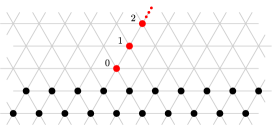
Figure 5: Worst-case configuration concerning work. The object particles are shown in black and the non-object particles are shown in red. The infinite object is a half-plane and the $n$ non-object particles lie on a straight line.

The particle labeled $i$ requires at least $2i$ movements before it lies contracted on the surface. Therefore, any algorithm requires at least $\sum_{i=0}^{n-1}2i=\Omega(n^{2})$ work. $\sqcap$$\sqcup$

Theorem 2

Our algorithm requires worst-case optimal work $\Theta(n^{2})$.

Proof.  To prove the upper bound, we simply show that every particle executes $O(n)$ movements. The theorem then follows by Lemma 5. Consider a particle $p$. While $p$ is inactive, it does not move. While $p$ is a follower, it moves along a path to the surface as described in the proof of Theorem 1. The length of this path is bound by $2n$ and, therefore, the number of movements $p$ executes while being a follower is $O(n)$. While $p$ is a leader it only performs expansions if it reads a complaint indicator. Since a complaint indicator is consumed by an expansion (see Section 5.2.3), a leader can see at most $n-1$ indicators. Every expansion is followed by a contraction, therefore the number of movements $p$ executes while being a leader is as well $O(n)$, which concludes the theorem. $\sqcap$$\sqcup$

6 Conclusion

In this work we have formally defined the Amoebot model and presented a work-optimal algorithm for the Infinite Object Coating problem under this model. We want to use the Amoebot model to investigate various other problems in which the system of particles forms a single connected component at all times. Other coating problems might be considered, in particular when the object surface is finite and the surface of an object has to be coated as uniformly as possible by the particles of a system (possibly with multiple layers of “coating”). A second example is the class of shape formation problems in which a system has to arrange to form a specific shape, with or without a seed particle. Finally, in bridging problems particles have to bridge gaps in given structures. We see the coating as an algorithmic primitive for solving other problems. For example, the formation of a shape can be achieved by creating an initially small instance of that shape which is then iteratively coated to form increasingly large instances until the number of particles in the system is exhausted. Furthermore, we envision that our spanning forest algorithm (Section 5.2.2) may in turn be a building block for other variations of the coating problems.

References

- [1] L. M. Adleman. Molecular computation of solutions to combinatorial problems. Science, 266(11):1021–1024, 1994.
- [2] Chrysovalandis Agathangelou, Chryssis Georgiou, and Marios Mavronicolas. A distributed algorithm for gathering many fat mobile robots in the plane. In Proceedings of the 2013 ACM symposium on Principles of distributed computing, pages 250–259. ACM, 2013.
- [3] R. Ananthakrishnan and A. Ehrlicher. The forces behind cell movement. International Journal of Biological Sciences, 3(5):303–317, 2007.
- [4] D. Angluin, J. Aspnes, Z. Diamadi, M. J. Fischer, and R. Peralta. Computation in networks of passively mobile finite-state sensors. Distributed Computing, 18(4):235–253, 2006.
- [5] D. Arbuckle and A. Requicha. Self-assembly and self-repair of arbitrary shapes by a swarm of reactive robots: algorithms and simulations. Autonomous Robots, 28(2):197–211, 2010.
- [6] Albert-Laszlo Barabasi and Reka Albert. Emergence of scaling in random networks. Science, 286(5439):509–512, 1999.
- [7] L. Barriere, P. Flocchini, E. Mesa-Barrameda, and N. Santoro. Uniform scattering of autonomous mobile robots in a grid. Int. Journal of Foundations of Computer Science, 22(3):679–697, 2011.
- [8] Y. Benenson, T. Paz-Elizur, R. Adar, E. Keinan, Z. Livneh, and E. Shapiro. Programmable and autonomous computing machine made of biomolecules. Nature, 414(6862):430–434, 2001.
- [9] A. Bhattacharyya, M. Braverman, B. Chazelle, and H.L. Nguyen. On the convergence of the hegselmann-krause system. CoRR, abs/1211.1909, 2012.
- [10] D. Boneh, C. Dunworth, R. J. Lipton, and J. Sgall. On the computational power of DNA. Discrete Applied Mathematics, 71:79–94, 1996.
- [11] V. Bonifaci, K. Mehlhorn, and G. Varma. Physarum can compute shortest paths. In Proceedings of SODA ’12, pages 233–240, 2012.
- [12] Z. J. Butler, K. Kotay, D. Rus, and K. Tomita. Generic decentralized control for lattice-based self-reconfigurable robots. International Journal of Robotics Research, 23(9):919–937, 2004.
- [13] B. Chazelle. Natural algorithms. In Proc. of ACM-SIAM SODA, pages 422–431, 2009.
- [14] K. C. Cheung, E. D. Demaine, J. R. Bachrach, and S. Griffith. Programmable assembly with universally foldable strings (moteins). IEEE Transactions on Robotics, 27(4):718–729, 2011.
- [15] G. Chirikjian. Kinematics of a metamorphic robotic system. In Proceedings of ICRA ’94, volume 1, pages 449–455, 1994.
- [16] Mark Cieliebak, Paola Flocchini, Giuseppe Prencipe, and Nicola Santoro. Distributed computing by mobile robots: Gathering. SIAM Journal on Computing, 41(4):829–879, 2012.
- [17] R. Cohen and D. Peleg. Local spreading algorithms for autonomous robot systems. Theoretical Computer Science, 399(1-2):71–82, 2008.
- [18] S. Das, P. Flocchini, N. Santoro, and M. Yamashita. On the computational power of oblivious robots: forming a series of geometric patterns. In Proceedings of 29th ACM Symposium on Principles of Distributed Computing (PODC), 2010.
- [19] X. Defago and S. Souissi. Non-uniform circle formation algorithm for oblivious mobile robots with convergence toward uniformity. Theoretical Computer Science, 396(1-3):97–112, 2008.
- [20] E. D. Demaine, M. J. Patitz, R. T. Schweller, and S. M. Summers. Self-assembly of arbitrary shapes using rnase enzymes: Meeting the kolmogorov bound with small scale factor (extended abstract). In Proceedings of STACS ’11, pages 201–212, 2011.
- [21] Zahra Derakhshandeh, Shlomi Dolev, Robert Gmyr, Andréa W. Richa, Christian Scheideler, and Thim Strothmann. Brief announcement: amoebot - a new model for programmable matter. In 26th ACM Symposium on Parallelism in Algorithms and Architectures, SPAA ’14, Prague, Czech Republic - June 23 - 25, 2014, pages 220–222, 2014.
- [22] Shlomi Dolev, Robert Gmyr, Andr a W. Richa, and Christian Scheideler. Ameba-inspired self-organizing particle systems. CoRR, abs/1307.4259, 2013.
- [23] Maximilian Drees, Martina Hüllmann, Andreas Koutsopoulos, and Christian Scheideler. Self-organizing particle systems. In IPDPS, pages 1272–1283, 2012.
- [24] Yuval Emek and Roger Wattenhofer. Stone age distributed computing. In Proceedings of the 2013 ACM symposium on Principles of distributed computing, pages 137–146. ACM, 2013.
- [25] S. Fekete, C. Gray, and A.Kroeller. Evacuation of rectilinear polygons. In Proceedings of the 4th International Conference Combinatorial Optimization and Applications (COCOA), pages 21–30, 2010.
- [26] S.P. Fekete and C. Schmidt. Polygon exploration with time-discrete vision. Computational Geometry, 43(2):148–168, 2010.
- [27] Paola Flocchini, David Ilcinkas, Andrzej Pelc, and Nicola Santoro. Computing without communicating: Ring exploration by asynchronous oblivious robots. Algorithmica, 65(3):562–583, 2013.
- [28] Paola Flocchini, Giuseppe Prencipe, Nicola Santoro, and Peter Widmayer. Arbitrary pattern formation by asynchronous, anonymous, oblivious robots. Theoretical Computer Science, 407(1):412–447, 2008.
- [29] T. Fukuda, S. Nakagawa, Y. Kawauchi, and M. Buss. Self organizing robots based on cell structures - cebot. In Proceedings of IROS ’88, pages 145–150, 1988.
- [30] T.-R. Hsiang, E. Arkin, M. Bender, S. Fekete, and J. Mitchell. Algorithms for rapidly dispersing robot swarms in unknown environments. In Proceedings of the 5th Workshop on Algorithmic Foundations of Robotics (WAFR), pages 77–94, 2002.
- [31] B. Katreniak. Biangular circle formation by asynchronous mobile robots. In Proceedings of the 12th International Colloquium on Structural Information and Communication Complexity (SIROCCO), pages 85–99, 2005.
- [32] S. Kernbach, editor. Handbook of Collective Robotics – Fundamentals and Challanges. Pan Stanford Publishing, 2012.
- [33] J. Kleinberg. The small-world phenomenon: an algorithmic perspective. In Proceedings of STOC ’00, pages 163–170, 2000.
- [34] P. Kling and F. Meyer auf der Heide. Convergence of local communication chain strategies via linear transformations. In Proceedings of the 23rd ACM Symposium on Parallelism in Algorithms and Architectures, pages 159–166, 2011.
- [35] T. Krasinski, S. Sakowski, and T. Poplawski. Autonomous push-down automaton built on dna. Informatica, 36:263–276, 2012.
- [36] K. Li, K. Thomas, C. Torres, L. Rossi, and C.-C. Shen. Slime mold inspired path formation protocol for wireless sensor networks. In Proceedings of ANTS ’10, pages 299–311, 2010.
- [37] J. McLurkin. Analysis and Implementation of Distributed Algorithms for Multi-Robot Systems. PhD thesis, Massachusetts Institute of Technology, 2008.
- [38] R. Nagpal, A. Kondacs, and C. Chang. Programming methodology for biologically-inspired self-assembling systems. Technical report, AAAI Spring Symposium on Computational Synthesis, 2003.
- [39] C. Parker and H. Zhang. Collective robotic site preparation. Adaptive Behavior, 14(1):5–19, 2006.
- [40] M. Rubenstein and W. Shen. Automatic scalable size selection for the shape of a distributed robotic collective. In Proc. of the IEEE/RSJ Intl. Conf. on Intelligent Robots and Systems (IROS), 2010.
- [41] Aaron Sterling. Distributed agreement in tile self-assembly. Natural Computing, 10(1):337–355, 2011.
- [42] Aaron D Sterling. A limit to the power of multiple nucleation in self-assembly. In Distributed Computing, pages 451–465. Springer, 2008.
- [43] I. Suzuki and M. Yamashita. Distributed anonymous mobile robots: Formation of geometric patterns. SIAM Journal on Computing, 28(4):1347–1363, 1999.
- [44] Tommaso Toffoli and Norman Margolus. Programmable matter: concepts and realization. Physica D: Nonlinear Phenomena, 47(1):263–272, 1991.
- [45] J. E. Walter, J. L. Welch, and N. M. Amato. Distributed reconfiguration of metamorphic robot chains. Distributed Computing, 17(2):171–189, 2004.
- [46] S. Watanabe, A. Tero, A. Takamatsu, and T. Nakagaki. Traffic optimization in railroad networks using an algorithm mimicking an amoeba-like organism, physarum plasmodium. Biosystems, 105(3):225–232, 2011.
- [47] D. J. Watts and S. H. Strogatz. Collective dynamics of ’small-world’ networks. Nature, 393(6684):440–442, 1998.
- [48] E. Winfree, F. Liu, L. A. Wenzler, and N. C. Seeman. Design and self-assembly of two-dimensional dna crystals. Nature, 394(6693):539–544, 1998.
- [49] Damien Woods, Ho-Lin Chen, Scott Goodfriend, Nadine Dabby, Erik Winfree, and Peng Yin. Active self-assembly of algorithmic shapes and patterns in polylogarithmic time. In ITCS, pages 353–354, 2013.
- [50] M. Yim, W.-M. Shen, B. Salemi, D. Rus, M. Moll, H. Lipson, E. Klavins, and G. S. Chirikjian. Modular self-reconfigurable robot systems. IEEE Robotics Automation Magazine, 14(1):43–52, 2007.