Testing a class of non-Kerr metrics with hot spots orbiting SgrA^∗

Abstract

SgrA^∗, the supermassive black hole candidate at the Galactic Center, exhibits flares in the X-ray, NIR, and sub-mm bands that may be interpreted within a hot spot model. Light curves and images of hot spots orbiting a black hole are affected by a number of special and general relativistic effects, and they can be potentially used to check whether the object is a Kerr black hole of general relativity. However, in a previous study we have shown that the relativistic features are usually subdominant with respect to the background noise and the model-dependent properties of the hot spot, and eventually it is at most possible to estimate the frequency of the innermost stable circular orbit. In this case, tests of the Kerr metric are only possible in combination with other measurements. In the present work, we consider a class of non-Kerr spacetimes in which the hot spot orbit may be outside the equatorial plane. These metrics are difficult to constrain from the study of accretion disks and indeed current X-ray observations of stellar-mass and supermassive black hole candidates cannot put interesting bounds. Here we show that near future observations of SgrA^∗ may do it. If the hot spot is sufficiently close to the massive object, the image affected by Doppler blueshift is brighter than the other one and this provides a specific observational signature in the hot spot’s centroid track. We conclude that accurate astrometric observations of SgrA^∗ with an instrument like GRAVITY should be able to test this class of metrics, except in the more unlikely case of a small viewing angle.

1 Introduction

SgrA^∗, the radio source associated to the 4 million Solar mass black hole (BH) candidate at the Galactic Center, exhibits powerful flares in the X-ray, near-infrared, and sub-millimeter bands [1, 2, 3, 4]. There are a few flares per day, during which the flux increases up to a factor 10. Every flare lasts 1-3 hours and has a quasi-periodic substructure with a time scale of about 20 minutes. These flares may be associated with blobs of plasma orbiting near the innermost stable circular orbit (ISCO) of SgrA^∗ [5], even if current observations cannot exclude other explanations [6, 7, 8]. The scenario of the blob of plasma is also supported by general relativistic magneto-hydrodynamic simulations of the accretion flow onto BHs. Temporary clumps of matter should indeed be common in the region near the ISCO radius [9, 10]. The presence of blobs of plasma orbiting close to SgrA^∗ will be soon tested by the GRAVITY instrument for the ESO Very Large Telescope Interferometer (VLTI) [11].

The scenario of a blob of plasma is usually refereed to as hot spot model and it has been extensively discussed in the case of the Kerr spacetime [5, 12, 13, 14]. Light curves and images of hot spots are strongly affected by the spacetime geometry around the BH and accurate measurements of the hot spot flux and polarization can potentially measure the spin of the central object [5]. In Ref. [15], two of us have expended these studies to the case of non-Kerr spacetimes to explore the possibility of using this kind of data to test the nature of SgrA^∗. The available X-ray data of stellar-mass and supermassive BH candidates can already be used to investigate whether these objects are the Kerr BHs of general relativity [16, 17, 18, 19, 20, 21, 22] (for a review, see e.g. [23, 24]), but there is a fundamental degeneracy between the estimate of the spin and of possible deviations from the Kerr geometry and with current observations it is impossible to confirm the Kerr BH paradigm [25, 26]. Only some exotic BH alternatives can be ruled out [27, 28, 29]. The same problem affects the observations of light curves of hot spots [15]. It turns out that the background noise and the model-dependent properties of the blob of plasma are more important than the relativistic features present in the light curves. In the most optimistic case in which we can claim that the hot spot is approximately at the ISCO radius, one can measure the ISCO frequency of the spacetime. In the case of a Kerr BH and with an independent estimate of the BH mass, there is a one-to-one correspondence between the ISCO frequency and the BH spin parameter $a_{*}$, and therefore it is possible to infer the value of the latter. If we relax the Kerr BH hypothesis, the ISCO frequency depends on both $a_{*}$ and possible deviations from the Kerr solution, with the result that it is only possible to constrain a combination of them. Such a degeneracy could be broken only in presence of other measurements of the spacetime geometry [15, 30, 31, 32, 33, 34].

In the present paper, we consider a class of non-Kerr spacetimes in which the blob of plasma may orbit the central object outside the equatorial plane. This is a quite general property when the massive body is more prolate than a Kerr BH with the same value of the spin parameter. Such a class of deformed objects is difficult to rule out with other techniques because they look like fast-rotating Kerr black holes [26, 35], and, even if the possibility is very speculative, some observations may even prefer them with respect to Kerr BHs [18, 19, 36, 37]. We also note that off-equatorial orbits may be possible even in the case of charged particles in Kerr spacetimes in presence of electromagnetic fields [38, 39, 40]. Our original idea was to figure out if such a scenario, which is qualitatively different from the Kerr case and the ones studied so far, has specific observational signatures in the radiation emitted by a hot spot and if present or future observations can test this class of spacetimes. We find that light curves and centroid tracks of hot spots orbiting in the vicinity of these non-Kerr BHs have indeed some peculiar properties, but the latter do not appear only in the case of off-equatorial orbits, but for any orbit sufficiently close to the BH and for certain viewing angles. More precisely, the hot spot’s light curve shows some peculiar features in the case of small inclination angles. This is unlikely the case of SgrA^∗, whose spin axis should probably be quite aligned with the one of the Galaxy and therefore our viewing angle can be expect to be large. An accurate measurement of the centroid track seems to be the key-point to test this class of metrics with SgrA^∗. Except in the case of a small inclination angle, the size of the centroid track is much smaller than the one expected in the case of the Kerr spacetime. While we here use a very simple hot spot model, we argue that the result is quite general. Such an observational signature in the centroid track is created by the image (either the primary or the secondary) affected by Doppler blueshift, which is brighter than the other one. The centroid track does not really track the orbit of the hot spot, but it is confined on the one side of the BH. The difference with the Kerr metric seems to be so large that the GRAVITY instrument should be able to distinguish the two scenarios. Accurate images of the hot spot might be able to determine if the hot spot’s orbit is above, on, or below the equatorial plane, but a definitive answer would require the study of more realistic hot spot models, which is beyond the scope of the present paper.

The content of the paper is as follows. In Section 2, we review the hot spot model. In Section 3, we present our scenario, in which the hot spot may orbit outside the equatorial plane. In Section 4, we compute light curves, images, and centroid tracks of hot spots in equatorial and off-equatorial orbits and we qualitatively compare these results with the predictions in the Kerr spacetime to check whether future observations can test this class of metrics. Summary and conclusions are in Section 5. Throughout the paper, we use units in which $G_{\rm N}=c=1$, unless stated otherwise.

2 Hot spot model

In this paper, we adopt a very simple model to describe a blob of plasma orbiting the BH. More accurate descriptions are necessarily model-dependent and current observations cannot really selected the best one. At the same time, the aim of this work is to figure out if there are qualitatively different features in the properties of the radiation emitted by a blob of plasma orbiting a certain class of non-Kerr BHs, either in equatorial and off-equatorial orbits. The goal is to figure out if present or future observations of SgrA^∗ can test these metrics. The calculation of the hot spot’s light curves and images consists of two parts, namely the one of the motion of the hot spot and the calculation of the propagation of the photons from the hot spot to the detector far from the compact object.

Here we model the blob of plasma as a geometrically thin region of finite area, in which all its points move with the same angular velocity $\Omega=d\phi/dt$. This is the standard hot model set-up, employed even in more sophisticated models. The 4-velocity of each point of the plasma is $u^{\mu}_{\rm spot}=(u^{t}_{\rm spot},0,0,\Omega u^{t}_{\rm spot})$. The spacetime is stationary and axisymmetric, so the line element can be written as

$$ds^{2}=g_{tt}dt^{2}+g_{rr}dr^{2}+g_{\theta\theta}d\theta^{2}+2g_{t\phi}dtd\phi+g_{\phi\phi}d\phi^{2}\,,$$ (2.1)

where the metric elements are independent of the $t$ and $\phi$ coordinates. From the normalization condition $g_{\mu\nu}u^{\mu}_{\rm spot}u^{\nu}_{\rm spot}=-1$, we have

$$u^{t}_{\rm spot}=\frac{1}{\sqrt{-g_{tt}-2\Omega g_{t\phi}-\Omega^{2}g_{\phi\phi}}}\,,$$ (2.2)

where the metric coefficients are calculated at the position of each point. The size of the hot spot cannot be too large, because otherwise some points may exceed the speed of light. It is sufficient to check that $g_{tt}+2\Omega g_{t\phi}+\Omega^{2}g_{\phi\phi}<0$ to avoid that this happens. Within our simple model, the emission of radiation is supposed to be isotropic and monochromatic. The hot spot is assumed optically thick and the local specific intensity of the radiation is described by a Gaussian distribution in the local Cartesian space

$$I_{\rm spot}(\nu_{\rm spot},x)\sim\delta(\nu_{\rm spot}-\nu_{\star})\exp\bigg{[}-\frac{|\textbf{\~{x}}-\textbf{\~{x}}_{\rm spot}(t)|^{2}}{2R^{2}_{\rm spot}}\bigg{]}\,,$$ (2.3)

where $\nu_{\rm spot}$ is the photon frequency measured in the rest-frame of the emitter and $\nu_{\star}$ is the emission frequency of this monochromatic source. The spatial position 3-vector x̃ is given in pseudo-Cartesian coordinates. Outside a distance of $4R_{\rm spot}$ from the guiding trajectory $\textbf{\~{x}}_{\rm spot}$, there is no emission. For more details, see Ref. [15].

The trajectories of the photons are more conveniently calculated backward in time, from the image plane of the distant observer to the orbital plane of the hot spot. The observer’s sky is divided into a number of small elements and the ray-tracing procedure provides the observed time-dependent flux density for each element. The photon with Cartesian coordinates $(X,Y)$ on the image plane of the distant observer and detected at the time $t_{\rm obs}$ has initial conditions $(t_{0},r_{0},\theta_{0},\phi_{0})$ given by

$$t_{0} =t_{\rm obs}\,,$$ (2.4)

$$r_{0} =\sqrt{X^{2}+Y^{2}+D^{2}}\,,$$ (2.5)

$$\theta_{0} =\arccos\frac{Y\sin i+D\cos i}{r_{0}}\,,$$ (2.6)

$$\phi_{0} =\arctan\frac{X}{D\sin i-Y\cos i}\,.$$ (2.7)

The initial 3-momentum of the photon, $\bf{k_{0}}$, must be perpendicular to the plane of the image of the observer. The initial conditions for the 4-momentum are thus

$$k^{r}_{0} =-\frac{D}{r_{0}}|\bf{k_{0}}|\,,$$ (2.8)

$$k^{\theta}_{0} =\frac{\cos i-(Y\sin i+D\sin i)\frac{D}{r_{0}^{2}}}{\sqrt{X^{2}+(D\sin i-Y\cos i)^{2}}}|\bf{k_{0}}|\,,$$ (2.9)

$$k^{\phi}_{0} =\frac{X\sin i}{X^{2}+(D\sin i-Y\cos i)^{2}}|\bf{k_{0}}|\,,$$ (2.10)

$$k^{t}_{0} =\sqrt{(k^{r}_{0})^{2}+r_{0}^{2}(k^{\theta}_{0})^{2}+r_{0}^{2}\sin^{2}\theta_{0}(k^{\phi}_{0})^{2}}\,,$$ (2.11)

where $D$ is the distance of the observer from the BH and $i$ is the observer line of sign with respect to the BH spin. The observer is located at the distance $D$ large enough that the background geometry is close to be flat and therefore $k^{t}_{0}$ can be inferred from the condition $g_{\mu\nu}k^{\mu}k^{\nu}=0$ with the metric tensor of a flat spacetime.

The photon trajectories are numerically integrated backward in time from the image plane of the distant observer to the point of the photon emission with the code used in Ref. [15]. The code solves the second-order photon geodesic equations by using the fourth-order Runge-Kutta-Nyström method, as in non-Kerr spacetimes the equations of motion in general are not separable and they cannot be reduced to first-order equations, as in Kerr. The specific intensity of the radiation measured by the distant observer is

$$I_{\rm obs}(\nu_{\rm obs},t_{\rm obs})=g^{3}I_{\rm spot}(\nu_{\rm spot},t_{\rm obs})\,,$$ (2.12)

where $g$ is the redshift factor

$$g=\frac{E_{\rm obs}}{E_{\rm spot}}=\frac{\nu_{\rm obs}}{\nu_{\rm spot}}=\frac{k_{\alpha}u^{\alpha}_{\rm obs}}{k_{\beta}u^{\beta}_{\rm spot}}\,,$$ (2.13)

$k^{\alpha}$ is the 4-momentum of the photon and $u_{\rm obs}^{\alpha}=(1,0,0,0)$ is the 4-velocity of the distant observer. $I_{\rm obs}(\nu_{\rm obs})/\nu^{3}_{\rm obs}=I_{\rm spot}(\nu_{\rm spot})/\nu^{3}_{\rm spot}$ follows from the Liouville theorem. Since the spacetime is stationary and axisymmetric, $k_{t}$ and $k_{\phi}$ are conserved. With the use of Eq. (2.2), we can write

$$g=\frac{\sqrt{-g_{tt}-2g_{t\phi}\Omega-g_{\phi\phi}\Omega^{2}}}{1+\lambda\Omega}\,,$$ (2.14)

where $\lambda=k_{\phi}/k_{t}$ is a constant and it can be evaluated on the plane of the distant observer. Doppler boosting and gravitational redshift are entirely encoded in the redshift factor $g$, while the effect of light bending is included by the ray-tracing calculation.

The photon flux measured by the distant observer is obtained after integrating $I_{\rm obs}$ over the solid angle subtended by the hot spot’s image on the observer’s sky

$$F(\nu_{\rm obs},t_{\rm obs})=\int I_{\rm obs}(\nu_{\rm obs},t_{\rm obs})\,\mathrm{d}\Omega_{\rm obs}=\int g^{3}I_{\rm spot}(\nu_{\rm spot},t_{\rm obs})\,\mathrm{d}\Omega_{\rm obs}\,.$$ (2.15)

The light curve (observed luminosity) is found integrating over the frequency range of the radiation

$$L(t_{\rm obs})=\int F(\nu_{\rm obs},t_{\rm obs})\,\mathrm{d}\nu_{\rm obs}\,.$$ (2.16)

Light curves and images of hot spots orbiting on the equatorial plane around Kerr and non-Kerr BHs for different values of the hot spot size, viewing angle, orbital radius, and parameters of the spacetime geometry can be seen in [15].

3 Non-Kerr spacetimes with hot spots in equatorial and off-equatorial orbits

In this paper, we consider the Johannsen-Psaltis (JP) metric [41], which describes the gravitational field around non-Kerr BHs and the deviations from the Kerr geometry are quantified by a set of “deformation parameters”. The simplest non-Kerr model has only one non-vanishing deformation parameter $\epsilon_{3}$. In Boyer-Lindquist coordinates, the line element reads [41]

$$ds^{2} = -\left(1-\frac{2Mr}{\Sigma}\right)\left(1+h\right)dt^{2}-\frac{4aMr\sin^{2}\theta}{\Sigma}\left(1+h\right)dtd\phi+\frac{\Sigma\left(1+h\right)}{\Delta+a^{2}h\sin^{2}\theta}dr^{2}+$$ (3.1)

$$+\Sigma d\theta^{2}+\left[\left(r^{2}+a^{2}+\frac{2a^{2}Mr\sin^{2}\theta}{\Sigma}\right)\sin^{2}\theta+\frac{a^{2}(\Sigma+2Mr)\sin^{4}\theta}{\Sigma}h\right]d\phi^{2}\,,$$

where $a=J/M$ is the specific BH angular momentum ($a_{*}=a/M$ is the dimensionless spin parameter), $\Sigma=r^{2}+a^{2}\cos^{2}\theta$, $\Delta=r^{2}-2Mr+a^{2}$, and

$$h=\frac{\epsilon_{3}M^{3}r}{\Sigma^{2}}\,.$$ (3.2)

The compact object is more prolate (oblate) than a Kerr BH with the same spin for $\epsilon_{3}>0$ ($\epsilon_{3}<0$); when $\epsilon_{3}=0$, we recover the Kerr solution.

In the Kerr background, equatorial circular orbits are always vertically stable, while they are radially stable only for radii larger than that of the ISCO. In a generic non-Kerr spacetime, equatorial circular orbits may also be vertically unstable and new phenomena may show up [42, 43, 44]. We note that these effects are not peculiar of the JP metric, but they seem to generically appear when the central object is more prolate than a Kerr BH with the same spin parameter. In the case of the JP metric, this requires that $\epsilon_{3}>0$ and that $a_{*}$ exceeds a critical value, which depends on $\epsilon_{3}$.

In hot spot models, the guiding trajectory of the blob of plasma can be assumed to follow the geodesics of the metric. However, more realistic models consider that the hot spot is not a point-like object and it is stretched by tidal forces, with the result that it becomes more like a very small toroidal accretion disk [5]. In what follows, we assume that the BH has a small thick accretion disk and that a sector of this disk is brighter. This is our hot spot. This model allows us to easily compute the trajectory, while we are not aware of a straightforward method to do the same in the case of off-equatorial geodesics. However, this is not a crucial assumption and we would have obtained the same conclusions within other models. We would like to remind the reader that the hot spot model wants only to explain the flares of SgrA^∗ and the associated substructures. The hot optically thin flow around SgrA^∗ which is suggested by a number of different astrophysical measurements (X-ray, radio, IR) should still be there [45].

Thick disks in JP spacetimes have been studied in Ref. [42]. When $\epsilon_{3}>0$, toroidal disks outside the equatorial plane may be possible. Within the Polish doughnut model [46, 47], the specific energy of the fluid element, $-u_{t}$, its angular velocity, $\Omega$, and its angular momentum per unit energy, $\lambda=-u_{\phi}/u_{t}$, are related by

$$u_{t}=-\sqrt{\frac{g^{2}_{t\phi}-g_{tt}g_{\phi\phi}}{g_{\phi\phi}+2\lambda g_{t\phi}+\lambda^{2}g_{tt}}}\,,\quad\Omega=-\frac{\lambda g_{tt}+g_{t\phi}}{\lambda g_{t\phi}+g_{\phi\phi}}\,,\quad\lambda=-\frac{g_{t\phi}+\Omega g_{\phi\phi}}{g_{tt}+\Omega g_{t\phi}}\,,$$ (3.3)

where $\lambda$ is conserved for a stationary and axisymmetric flow in a stationary and axisymmetric spacetime [46]. The simplest Polish doughnut model has $\lambda$ constant and it is the case studied in Ref. [42]. Within this set-up, it was found that toroidal disks are not on the equatorial plane when $\lambda_{1}<\lambda<\lambda_{\rm ISCO}$, where $\lambda_{1}$ is a critical value of the specific fluid angular momentum which depends on $a_{*}$ and $\epsilon_{3}$, while $\lambda_{\rm ISCO}$ is the specific angular momentum for a test-particle at the ISCO radius. For $\lambda>\lambda_{\rm ISCO}$, the disk is on the equatorial plane, while there is no accretion disk when $\lambda<\lambda_{1}$. We stress again that this is not a peculiar feature of the JP metric. For instance, the same phenomena was found in [43] for the Manko-Novikov spacetime, which is an exact solution of the vacuum Einstein’s equations (it avoids the no-hair theorem because the event horizon is not regular). The orbit of the hot spot is at the minimum of the potential of the thick disk [42]. When $\lambda>\lambda_{\rm ISCO}$, the hot spot’s orbit is on the equatorial plane, like in Kerr. For $\lambda<\lambda_{\rm ISCO}$, there is no disk in the Kerr spacetime, but a disk still exists for suitable $a_{*}$ and positive $\epsilon_{3}$ if $\lambda>\lambda_{1}$.

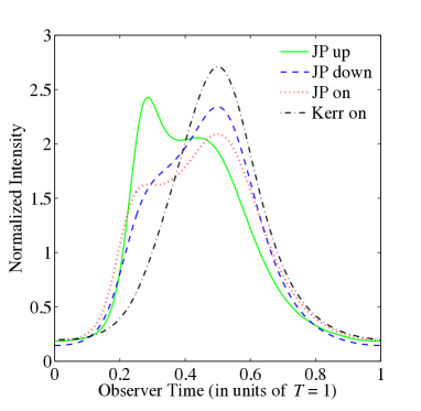
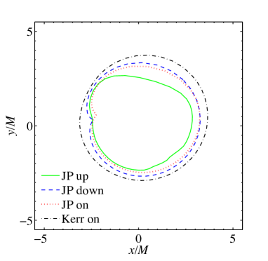
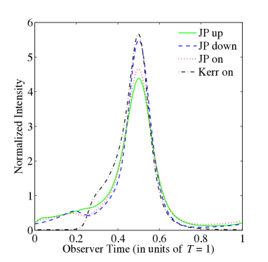
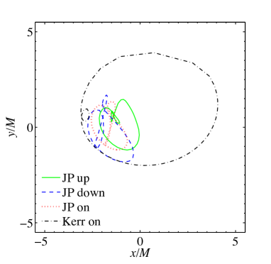
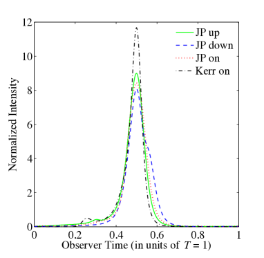
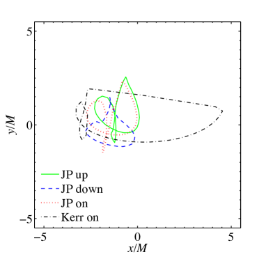
Figure 1: Light curves (left panels) and centroid tracks (right panels) of hot spots orbiting a JP BH above the equatorial plane (solid green curves), below the equatorial plane (dashed blue curves), and on the equatorial plane (dotted red curves) and a Kerr BH (dashed-dotted black curves). The viewing angle is $i=20^{\circ}$ (top panels), $45^{\circ}$ (central panels), and $70^{\circ}$ (bottom panels). The JP BH has $a_{*}=0.9$ and $\epsilon_{3}=2$. The Kerr BH has $a_{*}=0.9$. See the text for more details.

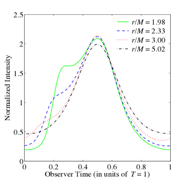
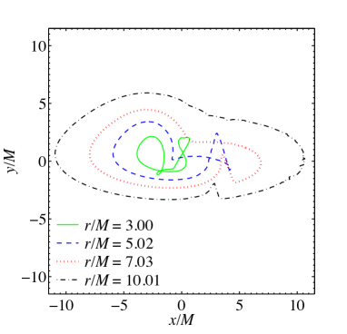
Figure 2: Light curves for a viewing angle $i=20^{\circ}$ (left panel) and centroid tracks for a viewing angle $i=70^{\circ}$ (right panel) of hot spots in equatorial orbits around a JP BH with $a_{*}=0.9$ and $\epsilon_{3}=2$. As the orbital radius $r$ increases, the observational signatures of this class of non-Kerr spacetimes disappears. In the light curve, the feature is not very prominent and it is already very weak when $r/M=3.00$. The feature in the centroid track is still evident for the case $r/M=3.00$, in which the hot spot orbital period would be about 14 minutes for SgrA^∗. See the text for more details.

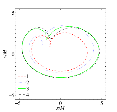
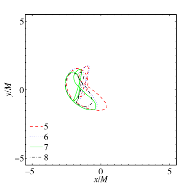
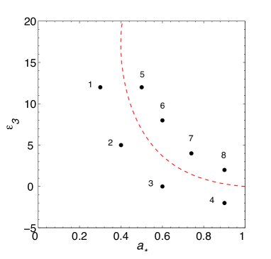
Figure 3: Centroid tracks for a viewing angle $i=45^{\circ}$ (top panels) of hot spots orbiting the JP BHs indicated in the bottom panel. In all these models, $\lambda=\lambda_{\rm ISCO}$. The red dashed curve on the spin parameter–deformation parameter plane separates spacetimes in which the ISCO radius is marginally radially stable (on the left) and marginally vertically unstable (on the right). Such a curve can be used as a general guide to distinguish models in which the centroid track is qualitatively similar to the one in the Kerr spacetime from the spacetimes in which the centroid track is small and dominated by the blueshifted image. See the text for more details.

4 Simulations

With the hot spot model described in Sections 2 and 3, we have computed light curves, images, and centroid tracks of blobs of plasma orbiting Kerr and JP BHs. If SgrA^∗ is a Kerr BH, the ISCO period should be between $\sim 30$ minutes ($a_{*}=0$) and $\sim 4$ minutes ($a_{*}=1$ and corotating orbit). The observed period of the quasiperiodic substructure of the flares of SgrA^∗ are around 20 minutes, with the shortest period ever measured of $13\pm 2$ minutes. The orbital radius of the hot spot may thus vary and be larger than that of the ISCO.

We now consider four hot spot models as illustrative examples: a hot spot around a Kerr BH and three hot spots around a JP BH in an orbit on, above, and below the equatorial plane. The orbital period in the four models is 8-9 minutes, which is not far from the current shortest period ever measured. For the Kerr model, we consider a BH with $a_{*}=0.9$. The hot spot’s orbit is clearly on the equatorial plane. We choose the fluid angular momentum per unit energy to be $\lambda=2.5$, which places the minimum of the potential of the disk and the hot spot’s orbital radius at $r/M=2.321$. For the JP models, we consider a BH with $a_{*}=0.9$ and $\epsilon_{3}=2$. In the case of the orbit on the equatorial plane, we choose $\lambda=1.291$, which makes the orbital radius at the radial coordinate $r/M=1.976$. For the orbits above and below the equatorial plane, we require $\lambda=1.28$ and we find that the radial coordinate of the orbit is $r/M=1.782$ and the height of the orbit from the equatorial plane is $z/M=0.69$. In the four models, the physical radius of the hot spot is $R_{\rm spot}=0.15$ $M$.

Fig. 1 shows the light curves (left panels) and the centroid tracks (right panels) of the four models for a viewing angle $i=20^{\circ}$ (top panels), $45^{\circ}$ (central panels), and $70^{\circ}$ (bottom panels). Even without a quantitative analysis, we can realize that the relativistic features encoded in the light curves for $i=45^{\circ}$ and $i=70^{\circ}$ are smaller than the error bars of the measurement and the background noise observed in the substructures of the flares of SgrA^∗ (see e.g. Figs. 8 and 11 in Ref. [5]). We find thus the same situation as in the hot spot models studied in Ref. [15]. For $i=20^{\circ}$, the light curve of the JP models has not a sinusoidal shape, but presents two bumps. This feature is more pronounced for the hot spot above the equatorial plane and less clear in the case of an orbit below the equatorial plane. This feature has never been observed in the substructures of the flares of SgrA^∗. However, it is unlikely that our viewing angle is small, as the spin of SgrA^∗ is more likely quite aligned with the axis of the Galaxy. Moreover, such a feature is not really prominent, so it is possible that it disappears within a different and more realistic hot spot model.

The centroid tracks of the four models are shown in the right panels in Fig. 1. The centroid is the center of emission on the observer’s sky and it has Cartesian coordinates

$$X_{\rm centr}(t_{\rm obs}) = \frac{1}{L(t_{\rm obs})}\int X\,I_{\rm obs}(\nu_{\rm obs},t_{\rm obs})\,\mathrm{d}\nu_{\rm obs}\,\mathrm{d}X\mathrm{d}Y\,,$$

$$Y_{\rm centr}(t_{\rm obs}) = \frac{1}{L(t_{\rm obs})}\int Y\,I_{\rm obs}(\nu_{\rm obs},t_{\rm obs})\,\mathrm{d}\nu_{\rm obs}\,\mathrm{d}X\mathrm{d}Y\,.$$ (4.1)

The centroid track is the curve $(X_{\rm centr}(t_{\rm obs}),Y_{\rm centr}(t_{\rm obs}))$ on the image plane of the distant observer. Again, a qualitative analysis is sufficient to realize that the centroid tracks in Kerr and JP background are quite similar for $i=20^{\circ}$. Here we note that an instrument like GRAVITY is supposed to provide astrometric measurements with an accuracy of about $M$. The cases with higher inclination angles are more interesting, even because they more likely reflect the true situation for SgrA^∗. It is evident that the size of the centroid tracks in the three JP models is dramatically smaller than the one expected for a hot spot orbiting a Kerr BH. A deeper investigation reveals that the feature is created by the image affected by Doppler blueshift, which is always brighter than the one affected by Doppler redshift. This is true even when the former is the secondary image and the latter is the primary one. The result is that the centroid track is confined in a smaller area around the image affected by Doppler blueshift, in our simulation on the left side of the BH, namely for $x/M<0$. We note that this can really represent an observational signature to rule out this class of spacetimes and it can unlikely disappear for different hot spot models: it is just the result of light bending created by the background geometry and it reflects the relative contribution in the total luminosity between the primary and the secondary images during an orbital period. Of course, the feature disappears for very small inclination angles, as in these cases the Doppler effect becomes negligible.

In the four models discussed, the hot spot is quite close to the BH, being its orbital period somewhat shorter than the shortest period of the flare’s quasiperiodic substructure ever observed in SgrA^∗. This fact would enhance the relativistic effects encoded in the light curves and the centroid tracks of the hot spot. What happens for hot spots at larger radii? To address this question, we have performed other simulations in the same background geometry, namely a JP BH with $a_{*}=0.9$ and $\epsilon_{3}=2$, but setting the hot spot at a larger orbital radius. The results are reported in Fig. 2. As the hot spot’s orbital radius increases, the relativistic signatures disappear, as they should do. In the case of the centroid tracks, the feature is still very clear for $r/M=3.00$ ($\lambda=2.10$). The orbital period of this hot spot would be about 14 minutes, which is a very reasonable time for a hot spot orbiting SgrA^∗. When $r/M=5.02$ ($\lambda=2.70$), the feature disappears and the centroid track covers a larger area, extending to the region $x/M>0$. In this case, the orbital period would be about 26 minutes.

Lastly, we want to show that such a non-Kerr signature belongs to a class of non-Kerr metrics, not just to the case with $\epsilon_{3}=2$. Fig. 3 shows the centroid tracks of four JP BHs in which there are no off-equatorial orbits (BHs 1-4) and of four JP BHs in which there are off-equatorial orbits (BHs 5-8). The red dashed line in the bottom panel is the boundary on the spin parameter–deformation parameter plane between spacetimes in which the ISCO radius is marginally radially (on the left of the red dashed line) and vertically (on the right) stable, which is also the boundary between spacetime without (on the left) and with (on the right) off-equatorial orbits. Such a red dashed line has however to be taken as a general guide. The transition from the centroid tracks of the kind in the top left panel to those in the top right panel is smooth. Moreover, for very large $\epsilon_{3}$ or in the right region but far from the red solid line, the spacetimes show pathological features and the picture is more complicated. We note that BH metrics just on the right of the red solid lines are difficult to constrain from the study of accretion disks and indeed current X-ray observations of stellar-mass and supermassive black hole candidates cannot put interesting bounds [26, 35]. The possible observation of hot spot orbiting SgrA^∗ seems to be able to do it.

In conclusion, we have provided the first explicit examples of non-Kerr metrics that can be realistically tested with GRAVITY. In general, as shown in Ref. [15], the difference between the predictions in the Kerr spacetime and in other backgrounds are too small and at least accurate observations of the position of the secondary images are necessary [48]. In the class of metrics considered in this paper, we have found a clear observational feature which can be identified by an instrument like GRAVITY. We have maintained our analysis strictly qualitative, because the aim of this work was to find a peculiar feature that can be detected independently of the hot spot model under consideration. Of course, the presence and the size of this feature eventually depend on $a_{*}$, $\epsilon_{3}$, and the orbital radius of the hot spot. Here we just claim that, for suitable parameters and a plausible viewing angle, such an observational signature could be strong enough to be detected, or otherwise the scenario may be ruled out.

5 Summary and conclusions

The radiation emitted by a blob of plasma orbiting a BH is affected by special and general relativistic effects and the observation of light curves and images of hot spots can potentially provide a number of important information about the spacetime geometry around the compact object. It is however disappointing that relativistic features play a minor role with respect to the specific model-dependent properties of the hot spot and that even the same background noise is usually dominant and washes out the information on the spacetime geometry. In the end, one can at most measure the frequency of the ISCO of the spacetime and it is not really possible to use these data to test whether astrophysical BH candidates are the Kerr BHs of general relativity [15].

In the present paper, we planned to explore a less ambitious idea. In the Kerr metric, blobs of plasma are expected to orbit the BH on the equatorial plane. In non-Kerr backgrounds, new phenomena may show up and off-equatorial orbits very close to the compact object are possible. As shown in previous studies, accretion disks in spacetimes with similar properties can look like disks around fast-rotating Kerr black holes and are difficult to test. Here we have investigated if these metrics can have observational signatures in the light curves and in the images of the blob of plasma and thus if it is possible to test the class of metrics presenting this feature with the observation of a hot spot in a similar situation. The main candidate for similar observations is SgrA^∗, the supermassive BH candidate at the Galactic Center. Its flares in the X-ray, NIR, and sub-mm bands may be interpreted within a hot spot model and in this case light curve data are already available. The measurement of hot spot centroid tracks could be possible in the near future with the GRAVITY instrument for the ESO VLTI. We actually find that specific signatures of these hot spots do not only belong to the ones in off-equatorial orbits, but to all the hot spots orbiting in the vicinity of the class of non-Kerr BHs in which such a non-equatorial orbits are possible.

For a large viewing angle, the signature of these geometries in the light curve is small, and it does not seem possible to test the spacetime with these observations. For a small viewing angle, the light curve carries a more pronounced feature (see the top left panel in Fig. 1). For sure, these features are not observed in present data. However, there is a number of caveats. The angle between our line of sight and the spin of SgrA^∗ is currently unknown, but it should be expected to be large. Actual data have a complicated structure and the feature found in our simple model is not so large, so in a more realistic model it may be subdominant with respect to the background noise. Observations suggest that the hot spot radius is variable and is larger than the ISCO one, so we may not be yet so lucky to have observed a hot spot sufficiently closed to the BH.

The observation of the centroid track seems to be a more promising technique to test this class of spacetimes. Except in the case of a small inclination angle, the hot spot’s centroid track is substantially different from the one expected in the Kerr case. The image affected by Doppler blueshift is brighter than the other one, even when the former is the secondary image and the latter is the primary one. Such a strong light bending produces a peculiar feature in the centroid track, which is actually confined on the one side of the BH and its size is much smaller than the one expected from a hot spot orbiting a Kerr BH. Even if we have performed the calculations in a very simple hot spot model, we do not expect that the effect disappear in the case of a more realistic set-up, because it arises from the relative contribution between the primary and secondary images, independently of the size, the shape, and the emission properties of the hot spot.

References

- [1] R. Genzel, R. Schodel, T. Ott, A. Eckart, T. Alexander, F. Lacombe, D. Rouan and B. Aschenbach, Nature 425, 934 (2003) [astro-ph/0310821].
- [2] A. M. Ghez, S. A. Wright, K. Matthews, D. Thompson, D. Le Mignant, A. Tanner, S. D. Hornstein and M. Morris et al., Astrophys. J. 601, L159 (2004) [astro-ph/0309076].
- [3] K. Dodds-Eden, S. Gillessen, T. K. Fritz, F. Eisenhauer, S. Trippe, R. Genzel, T. Ott and H. Bartko et al., Astrophys. J. 728, 37 (2011) [arXiv:1008.1984 [astro-ph.GA]].
- [4] G. Trap, A. Goldwurm, K. Dodds-Eden, A. Weiss, R. Terrier, G. Ponti, S. Gillessen and R. Genzel et al., Astron. Astrophys. 528, 140 (2011) [arXiv:1102.0192 [astro-ph.HE]].
- [5] N. Hamaus, T. Paumard, T. Muller, S. Gillessen, F. Eisenhauer, S. Trippe and R. Genzel, Astrophys. J. 692, 902 (2009) [arXiv:0810.4947 [astro-ph]].
- [6] S. Markoff, H. Falcke, F. Yuan and P. L. Biermann, Astron. Astrophys. 379, L13 (2001) [astro-ph/0109081].
- [7] M. Tagger and F. Melia, Astrophys. J. 636, L33 (2006) [astro-ph/0511520].
- [8] F. Yusef-Zadeh, D. Roberts, M. Wardle, C. O. Heinke and G. C. Bower, Astrophys. J. 650, 189 (2006) [astro-ph/0603685].
- [9] J. P. De Villiers, J. F. Hawley and J. H. Krolik, Astrophys. J. 599, 1238 (2003) [astro-ph/0307260].
- [10] J. D. Schnittman, J. H. Krolik and J. F. Hawley, Astrophys. J. 651, 1031 (2006) [astro-ph/0606615].
- [11] F. Eisenhauer, G. Perrin, W. Brandner, C. Straubmeier, A. Richichi, S. Gillessen, J. P. Berger and S. Hippler et al., arXiv:0808.0063 [astro-ph].
- [12] J. D. Schnittman and E. Bertschinger, Astron. Astrophys. 606, 1098 (2004) [astro-ph/0309458].
- [13] J. D. Schnittman, Astrophys. J. 621, 940 (2005) [astro-ph/0407179].
- [14] A. E. Broderick and A. Loeb, Mon. Not. Roy. Astron. Soc. 363, 353 (2005) [astro-ph/0506433].
- [15] Z. Li, L. Kong and C. Bambi, Astrophys. J. 787, 152 (2014) [arXiv:1401.1282 [gr-qc]].
- [16] C. Bambi and E. Barausse, Astrophys. J. 731, 121 (2011) [arXiv:1012.2007 [gr-qc]].
- [17] C. Bambi, Phys. Rev. D 85, 043002 (2012) [arXiv:1201.1638 [gr-qc]].
- [18] C. Bambi, Phys. Rev. D 86, 123013 (2012) [arXiv:1204.6395 [gr-qc]].
- [19] C. Bambi, JCAP 1209, 014 (2012) [arXiv:1205.6348 [gr-qc]].
- [20] C. Bambi, Astrophys. J. 761, 174 (2012) [arXiv:1210.5679 [gr-qc]].
- [21] C. Bambi, Phys. Rev. D 87, 023007 (2013) [arXiv:1211.2513 [gr-qc]].
- [22] T. Johannsen and D. Psaltis, Astrophys. J. 773, 57 (2013) [arXiv:1202.6069 [astro-ph.HE]].
- [23] C. Bambi, Mod. Phys. Lett. A 26, 2453 (2011) [arXiv:1109.4256 [gr-qc]].
- [24] C. Bambi, Astron. Rev. 8, 4 (2013) [arXiv:1301.0361 [gr-qc]].
- [25] C. Bambi, JCAP 1308, 055 (2013) [arXiv:1305.5409 [gr-qc]].
- [26] L. Kong, Z. Li and C. Bambi, Astrophys. J. 797, 78 (2014) [arXiv:1405.1508 [gr-qc]].
- [27] C. Bambi, Phys. Rev. D 87, no. 8, 084039 (2013) [arXiv:1303.0624 [gr-qc]].
- [28] P. S. Joshi, D. Malafarina and R. Narayan, Class. Quant. Grav. 31, 015002 (2014) [arXiv:1304.7331 [gr-qc]].
- [29] C. Bambi and D. Malafarina, Phys. Rev. D 88, 064022 (2013) [arXiv:1307.2106 [gr-qc]].
- [30] C. Bambi and K. Freese, Phys. Rev. D 79, 043002 (2009) [arXiv:0812.1328 [astro-ph]].
- [31] C. Bambi and N. Yoshida, Class. Quant. Grav. 27, 205006 (2010) [arXiv:1004.3149 [gr-qc]].
- [32] N. Tsukamoto, Z. Li and C. Bambi, JCAP 1406, 043 (2014) [arXiv:1403.0371 [gr-qc]].
- [33] C. Bambi, arXiv:1409.0310 [gr-qc].
- [34] D. Psaltis, F. Ozel, C. K. Chan and D. P. Marrone, arXiv:1411.1454 [astro-ph.HE].
- [35] C. Bambi, Phys. Lett. B 705, 5 (2011) [arXiv:1110.0687 [gr-qc]].
- [36] C. Bambi, arXiv:1312.2228 [gr-qc].
- [37] C. Bambi, arXiv:1412.4987 [gr-qc].
- [38] J. Kovar, Z. Stuchlik and V. Karas, Class. Quant. Grav. 25, 095011 (2008) [arXiv:0803.3155 [astro-ph]].
- [39] J. Kovar, O. Kopacek, V. Karas and Z. Stuchlik, Class. Quant. Grav. 27, 135006 (2010) [arXiv:1005.3270 [astro-ph.HE]].
- [40] C. Cremaschini, J. Kova, P. Slan, Z. Stuchlik and V. Karas, Astrophys. J. Suppl. 209, 15 (2013) [arXiv:1309.3979 [astro-ph.HE]].
- [41] T. Johannsen and D. Psaltis, Phys. Rev. D 83, 124015 (2011) [arXiv:1105.3191 [gr-qc]].
- [42] Z. Li and C. Bambi, JCAP 1303, 031 (2013) [arXiv:1212.5848 [gr-qc]].
- [43] C. Bambi and E. Barausse, Phys. Rev. D 84, 084034 (2011) [arXiv:1108.4740 [gr-qc]].
- [44] C. Bambi and L. Modesto, Phys. Lett. B 706, 13 (2011) [arXiv:1107.4337 [gr-qc]].
- [45] F. Yuan and R. Narayan, Ann. Rev. Astron. Astrophys. 52, 529 (2014) [arXiv:1401.0586 [astro-ph.HE]].
- [46] M. Kozlowski, M. Jaroszynski and M. Abramowicz, Astron. Astrophys. 63, 209 (1978).
- [47] M. Abramowicz, M. Jaroszynski and M. Sikora, Astron. Astrophys. 63, 221 (1978).
- [48] Z. Li and C. Bambi, Phys. Rev. D 90, 024071 (2014) [arXiv:1405.1883 [gr-qc]].
- [49] C. Bambi, Phys. Rev. D 87, 107501 (2013) [arXiv:1304.5691 [gr-qc]].