Independent sets and hitting sets of bicolored rectangular families

Abstract

A bicolored rectangular family BRF is a collection of all axis-parallel rectangles contained in a given region $\mathcal{Z}$ of the plane formed by selecting a bottom-left corner from a set $A$ and an upper-right corner from a set $B$. We prove that the maximum independent set and the minimum hitting set of a BRF have the same cardinality and devise polynomial time algorithms to compute both. As a direct consequence, we obtain the first polynomial time algorithm to compute minimum biclique covers, maximum cross-free matchings and jump numbers in a class of bipartite graphs that significantly extends convex bipartite graphs and interval bigraphs. We also establish several connections between our work and other seemingly unrelated problems. Furthermore, when the bicolored rectangular family is weighted, we show that the problem of finding the maximum weight of an independent set is $\mathbf{NP}$-hard, and provide efficient algorithms to solve it on certain subclasses.

1 Introduction

Suppose we are given a collection of axis-parallel closed rectangles in the plane. A subcollection of rectangles that do not pairwise intersect is called an independent set, and a collection of points in the plane intersecting (hitting) every rectangle is called a hitting set. In this paper we study the problems of finding a maximum independent set (MIS) and a minimum hitting set (MHS) of restricted classes of rectangles arising from bicolored point-sets in the plane, and relate them to other problems in graph and poset theory.

Both the MIS and its weighted version WMIS are important problems in computational geometry with a variety of applications [23, 38, 2, 33, 39]. Since MIS is $\mathbf{NP}$-hard [27, 36], a significant amount of research has been devoted to heuristics and approximation algorithms. Charlermsook and Chuzhoy [13], and Chalermsook [12] describe two different $O(\log\log m)$-approximation algorithms for the MIS problem on a family of $m$ rectangles, while Chan and Har-Peled [15] provide an $O(\log m/\log\log m)$-approximation factor for WMIS. The approximation factor achieved by these polynomial time algorithms are the best so far for general rectangle families. Nevertheless, very recently Adamaszek and Wiese [1] presented a pseudo-polynomial algorithm achieving a $(1+\varepsilon)$-approximation for WMIS in general rectangles. For special classes of rectangle families, the situation is better: there are polynomial time approximation schemes (PTAS) for MIS in squares [14], rectangles with bounded width to height ratio [24], rectangles of constant height [2], and rectangles forming a pseudo-disc family, that is, the intersection of the boundaries of any two rectangles consists of at most two points [3, 15].

The MHS problem is the dual of the MIS problem, and therefore the value of an optimal solution of MHS is an upper bound for that of MIS. The MHS problem is also $\mathbf{NP}$-hard [27], but there are also PTAS for special cases, including squares [14], rectangles of constant height [16] and pseudodiscs [46]. More recently, Aronov, Ezra, and Sharir [5] proved the existence of $\varepsilon$-nets of size $O(\frac{1}{\varepsilon}\log\log\frac{1}{\varepsilon})$ for axis-parallel rectangle families. Using Brönnimann and Goodrich’s technique [10], this yields an $O(\log\log\tau)$ approximation algorithm for any rectangle family that can be hit by at most $\tau$ points yielding the best approximation guarantee for MHS known.

1.1 Main results

In this article we study both the MIS and MHS problems on a special class of rectangle families. Given two finite sets $A,B\subseteq\mathbb{R}^{2}$ and an arbitrary set $\mathcal{Z}\subseteq\mathbb{R}^{2}$ of the plane, we define the bicolored rectangle family (BRF) induced by $A$, $B$ and $\mathcal{Z}$ as the set $\mathcal{R}=\mathcal{R}(A,B,\mathcal{Z})$ of all rectangles contained in $\mathcal{Z}$, having bottom-left corner in $A$ and top-right corner in $B$. When $\mathcal{Z}$ is the entire plane, we write $\mathcal{R}(A,B)$ and we call it an unrestricted BRF.

Our main result is an algorithm that simultaneously finds an independent set $I$ and a hitting set $H$ of $\mathcal{R}(A,B,\mathcal{Z})$ with $\lvert I\rvert=\lvert H\rvert$. By linear programming duality, $I$ and $H$ are a MIS and a MHS of $\mathcal{R}$, respectively; meaning in particular that we have a max-min relation between both quantities.

Our algorithm is efficient: if $n$ is the number of points in $A\cup B$, both the MIS and the MHS of $\mathcal{R}$ can be computed deterministically in $O(n^{2.5}\sqrt{\log n})$ time. If we allow randomization, we can compute them with high probability in time $O((n\log n)^{\omega})$, where $\omega<2.3727$ is the exponent of square matrix multiplication. Here we implicitly assume that testing if a rectangle is contained in $\mathcal{Z}$ can be done in unit time (by an oracle); otherwise, we need additional $O(n^{2}T(\mathcal{Z}))$ time, where $T(\mathcal{Z})$ is the time for testing membership in $\mathcal{Z}$. The bottleneck of our algorithm is the computation of a maximum matching on a bipartite graph needed for an algorithmic version of the classic Dilworth’s theorem.

We also show that a natural linear programming relaxation for the MIS of BRFs can be used to compute the optimal size of the maximum independent set. Using an uncrossing technique, we prove that one of the vertices in the optimal face of the underlying polytope is integral, and we show how to find that vertex efficiently. This structural result about this linear program relaxation gives a second algorithm to compute the maximum independent set of a BRF and should be of interest by itself.

1.2 Biclique covers, cross-free matchings and jump number

Our results have some consequences for two graph problems called the minimum biclique cover and the maximum cross-free matching. Before stating the relation we give some background on these problems.

A biclique of a bipartite graph is the edge set of a complete bipartite subgraph. A biclique cover is a collection of bicliques whose union is the entire edge set. Two edges $e$ and $f$ cross if there is a biclique containing both. A cross-free matching is a collection of pairwise non-crossing edges.

The problem of finding a minimum biclique cover arises in many areas (e.g. biology [47], chemistry [19] and communication complexity [37]). Orlin [48] has shown that finding a minimum biclique cover of a bipartite graph is $\mathbf{NP}$-hard. Müller [44] extended this result to chordal bipartite graphs. To our knowledge, the only classes of graphs for which this problem has been explicitly shown to be polynomially solvable before our work are $C_{4}$-free bipartite graphs [44], distance hereditary bipartite graphs [44], bipartite permutation graphs [44], domino-free bipartite graphs [4] and convex bipartite graphs [34, 32]. The proof of polynomiality for this last class can be deduced from the statement that the minimum biclique cover problem on convex bipartite graphs is equivalent to finding the minimum basis of a family of intervals. The latter was originally studied and solved by Győri [34], but its connection with the minimum biclique problem was only noted several years later [4] (See Section 6 for more details).

The maximum cross-free matching problem is often studied because of its relation to the jump number problem in Poset Theory. The jump number of a partial order $P$ with respect to a linear extension $L$ is the number of pairs of consecutive elements in $L$ that are incomparable in $P$. The jump number of $P$ is the minimum of this quantity over all linear extensions. Chaty and Chein [17] show that computing the jump number of a poset is equivalent to finding a maximum alternating-cycle-free matching in the underlying comparability graph, which is $\mathbf{NP}$-hard as shown by Pulleyblank [49]. For chordal bipartite graphs, alternating-cycle-free matching and cross-free matchings coincide, making the jump number problem equivalent to the maximum cross-free matching problem. Müller [43] has shown that this problem is $\mathbf{NP}$-hard for chordal bipartite graphs, but there are efficient algorithms to solve it on important subclasses. In order of inclusion, there are linear and cuadratic algorithms for bipartite permutation graphs [54, 8, 25], a cuadratic algorithm for biconvex graphs [8] and an $O(n^{9})$ time algorithm for convex bipartite graphs [22].

To relate our results with the problems just defined consider the following construction. Given a BRF $\mathcal{R}(A,B,\mathcal{Z})$, create a bipartite graph with vertex color classes $A$ and $B$ identifying every rectangle $R\in\mathcal{R}$ with bottom-left corner $a\in A$ and top-right corner $b\in B$ with an edge connecting $a$ and $b$. The resulting graph $G=(A\cup B,\mathcal{R})$ is the graph representation of $\mathcal{R}$. We call the graphs arising in this way BRF graphs.

It is an easy exercise to check that for an unrestricted BRF graph—i.e., a graph $G=(A\cup B,\mathcal{R})$ where $\mathcal{R}$ is unrestricted—two edges $R$ and $R^{\prime}$ cross if and only if $R$ and $R^{\prime}$ intersect as rectangles. In particular, the cross-free matchings of $G$ are in correspondence with the independent sets of $\mathcal{R}$. Similarly, the maximal bicliques of $G$ (in the sense of inclusion) are exactly the maximal families of pairwise intersecting rectangles in $\mathcal{R}$. Using the Helly property for axis-parallel rectangles we conclude that the minimum hitting set problem on $\mathcal{R}$ is equivalent to the minimum biclique cover of $G$.

Our results imply then that for unrestricted BRF graphs, the maximum size of a cross-free matching equals the minimum size of a biclique cover and both optimizers can be computed in polynomial time. Since unrestricted BRFs are chordal bipartite [51], we also obtain polynomial time algorithms to compute the jump number of unrestricted BRFs.

1.3 Additional results for the weighted case

We also consider the natural weighted version of MIS, denoted WMIS, where each rectangle in the family has a non-negative weight, and we aim to find a collection of disjoint rectangles with maximum total weight. For BRFs, this problem is equivalent to finding a maximum weight cross-free matching of the associated BRF graph.

We show that this problem is $\mathbf{NP}$-hard for unrestricted BRFs and weights in $\{0,1\}$. Afterwards, we present some results for certain subclasses. For bipartite permutation graphs, we provide an $O(n^{2})$ algorithm for arbitrary weights and a specialized $O(n)$ algorithm when weights are in $\{0,1\}$. We also note how the algorithm of Lubiw [41] for the maximum weight set of point-interval pairs readily translates into an algorithm for the WMIS of convex graphs that runs in $O(n^{3})$ time. Recent results of Correa et al. [21, 20] can be used to extend the $\mathbf{NP}$-hardness to interval bigraphs and to provide a 2-approximation algorithm for WMIS on this class.

1.4 Relation with other works

The min-max result relating independent sets and hitting sets in BRFs can also be obtained as a consequence of a deep duality result of Frank and Jordán for set-pairs [30]. Because of the many non-trivial connections between our work and other problems indirectly related to set-pairs, we defer the introduction of this concept and the discussion of these connections to Section 6, when all our results have been introduced. Although the min-max result is a consequence of an existent result, our algorithmic proof is significantly simpler than those for the larger class of set-pairs. And because of its geometrical nature, it is also more intuitive.

2 Preliminaries

We denote the coordinates of the plane $\mathbb{R}^{2}$ as $x$ and $y$, so that a point $p$ is written as $(p_{x},p_{y})$. Given two points $p$, $p^{\prime}\in\mathbb{R}^{2}$, we write $p\leq_{\mathbb{R}^{2}}p^{\prime}$ if and only if $p_{x}\leq p^{\prime}_{x}$ and $p_{y}\leq p^{\prime}_{y}$. For any set $S\subseteq\mathbb{R}^{2}$, the projection $\{s_{x}\colon s\in S\}$ of $S$ onto the $x$ axis is denoted by $S_{x}$. Given two sets $S$ and $S^{\prime}$ in $\mathbb{R}^{2}$, we write $S_{x}<S^{\prime}_{x}$ if the projection $S_{x}$ is to the left of the projection $S^{\prime}_{x}$, that is, if $p_{x}<p^{\prime}_{x}$ for all $p\in S$, $p^{\prime}\in S^{\prime}$. We extend this convention to $S_{x}>S^{\prime}_{x},S_{x}\leq S^{\prime}_{x}$ and $S_{x}\geq S^{\prime}_{x}$, as well as to the projections onto the $y$-axis. For our purposes, a rectangle $R$ is the cartesian product of two closed intervals. In other words, we only consider axis-parallel closed rectangles. We say that two rectangles $R$ and $R^{\prime}$ intersect if they have a non-empty geometric intersection. A point $p$ hits a rectangle $R$ if $p\in R$. A collection of pairwise non-intersecting rectangles is called an independent set of rectangles. A collection of points $H$ is a hitting set of a rectangle family $\mathcal{C}$ if each rectangle in $\mathcal{C}$ is hit by a point in $H$. We denote by $\mathbf{mis}(\mathcal{C})$ and $\mathbf{mhs}(\mathcal{C})$ the sizes of a maximum independent set of rectangles in $\mathcal{C}$ and a minimum hitting set for $\mathcal{C}$ respectively.

The intersection graph $\mathcal{I}(\mathcal{C})$ of a collection of rectangles $\mathcal{C}$ is the graph on $\mathcal{C}$ having edges between intersecting rectangles:

$$\mathcal{I}(\mathcal{C})\equiv(\mathcal{C},E),\quad\text{ where }E=\{RR^{\prime}\colon R\cap R^{\prime}\neq\emptyset\}.$$

Note that the independent sets of rectangles in $\mathcal{C}$ are exactly the stable sets of $\mathcal{I}(\mathcal{C})$. Furthermore, since $\mathcal{C}$ has the Helly property, we can assign to every clique in $\mathcal{I}(\mathcal{C})$ a unique witness point, defined as the leftmost and lowest point contained in all rectangles of the clique. Since different maximal cliques have different witness points, it is easy to prove that $\mathcal{C}$ admits a minimum hitting set consisting only of witness points of maximal cliques. In particular, $\mathbf{mhs}(\mathcal{C})$ equals the minimum size of a clique-cover of $\mathcal{I}(\mathcal{C})$.

For both MIS and MHS, we can restrict ourselves to the family $\mathcal{C}_{\downarrow}$ of inclusionwise minimal rectangles in $\mathcal{C}$: any maximum independent set in $\mathcal{C}_{\downarrow}$ is also maximum in $\mathcal{C}$ and any minimum hitting set for $\mathcal{C}_{\downarrow}$ is also minimum for $\mathcal{C}$. Since the size of every independent set is at most the size of any hitting set, we observe that for any family $\mathcal{C}$,

$$\mathbf{mis}(\mathcal{C}_{\downarrow})=\mathbf{mis}(\mathcal{C})\leq\mathbf{mhs}(\mathcal{C})=\mathbf{mhs}(\mathcal{C}_{\downarrow}).$$ (1)

2.1 Bicolored Rectangular Families (BRFs)

In what follows, let $A$ and $B$ be finite sets of white and gray points on the plane, respectively, and $\mathcal{Z}\subseteq\mathbb{R}^{2}$ be a set not necessarily finite.

We denote by $\Gamma(a,b)=\{p\in\mathbb{R}^{2}\colon a_{x}\leq p_{x}\leq b_{x},a_{y}\leq p_{y}\leq b_{y}\}$ the rectangle with bottom-left corner $a$ and upper-right corner $b$. The set

$$\mathcal{R}=\mathcal{R}(A,B,\mathcal{Z})=\{\Gamma(a,b)\colon a\in A,b\in B,a\leq_{\mathbb{R}^{2}}b\text{ and }\Gamma(a,b)\subseteq\mathcal{Z}\}$$

is called the bicolored rectangular family (BRF) associated to $(A,B,\mathcal{Z})$.

We denote $n=\lvert A\cup B\rvert$ and use $[k]$ to denote the set $\{1,2,\ldots,k\}$. To make the exposition simpler, we will assume without loss of generality that $A\cap B=\emptyset$, that $A\cup B\subseteq\mathcal{Z}$, that the points in $A\cup B$ have integral coordinates in $[n]\times[n]$, and that no two points of $A\cup B$ share a common coordinate value. Under these assumptions, we only need to consider hitting sets in $\mathcal{Z}\cap[n]^{2}$. We also assume that the set $\mathcal{Z}$ is given implicitly, i.e. its size is not part of the input, and that we can test if a rectangle is contained in $\mathcal{Z}$ either in unit time (using an oracle) or in a fixed time $T(\mathcal{Z})$.

A non-empty intersection between two rectangles $R$ and $S$ in $\mathcal{R}$ is called a corner intersection if either rectangle contains a vertex of the other rectangle in its interior. Otherwise, the intersection is called corner-free. A corner-free intersection (c.f.i.) family is a collection of rectangles such that every intersection is corner-free. These intersections are generically shown in Figure 1.

Figure 1: Corner-free intersections

Corner-free intersections families have a special structure, as the next proposition shows.

Proposition 2.1.

If $\mathcal{K}$ is a c.f.i. family then $\mathcal{I}(\mathcal{K})$ is a comparability graph.

Proof.

Consider the relation $\hookrightarrow$ on $\mathcal{K}$. given by $R\hookrightarrow S$ if and only if $R_{x}\subseteq S_{x}$ and $S_{y}\subseteq R_{y}$. It is easy to check that $\hookrightarrow$ is a partial order relation. Since $\mathcal{K}$ is a c.f.i. family, $R$ and $S$ intersect if and only if they are comparable under $\hookrightarrow$. Therefore $\mathcal{I}(\mathcal{K})$ is the comparability graph of $(\mathcal{K},\hookrightarrow$). ∎

The following lemma will also be useful later.

Lemma 2.2.

Every rectangle in $\mathcal{R}_{\downarrow}$ does not contain any point in $A\cup B$ other than its two defining corners.

Proof.

Direct. ∎

2.2 Comparability intersection graphs

Let $\mathcal{K}$ be a family of rectangles such that $\mathcal{I}(\mathcal{K})$ is the comparability graph of an arbitrary partial order $(\mathcal{K},\hookrightarrow)$. Independent sets in $\mathcal{K}$ correspond then to antichains in $(\mathcal{K},\hookrightarrow)$; therefore the maximum independent set problem in $\mathcal{K}$ is equivalent to the maximum cardinality antichain problem in $(\mathcal{K},\hookrightarrow)$.

Rectangles hit by a fixed point are trivially pairwise intersecting; therefore they are chains in $(\mathcal{K},\hookrightarrow)$. By the Helly property, any family of pairwise intersecting rectangles is hit by single point. It follows that finding a minimum hitting set of $\mathcal{K}$ is equivalent to finding a minimum size family of chains in $(\mathcal{K},\hookrightarrow)$ covering all the elements of $\mathcal{K}$. The latter is the description of the minimum chain covering problem.

Dilworth’s theorem states that for any partial order, the maximum cardinality of an antichain equals the size of a minimum chain cover. In our context, this directly translate to:

Lemma 2.3.

If $\mathcal{I}(\mathcal{K})$ is a comparability graph then $\mathbf{mis}(\mathcal{K})=\mathbf{mhs}(\mathcal{K})$.

From an algorithmic perspective, finding a maximum antichain and a minimum chain covering on a partial ordered set $\mathcal{K}$ can be done by computing a minimum vertex cover and a maximum matching on a bipartite graph (see, e.g. [26]). Since for bipartite graphs a minimum vertex cover can be obtained from a maximum matching in time proportional to the number of edges in the graph [50], the following result holds:

Lemma 2.4.

(See, e.g., [26]) The maximum antichain and the minimum chain covering of a partial order $\mathcal{K}$ can be found in $O(\operatorname{matching}(v,e))$, where $v$ is the number of elements in $\mathcal{K}$, $e$ is the number of pairs of comparable elements in $\mathcal{K}$, and $\operatorname{matching}(v,e)$ is the running time of an algorithm that solves the bipartite matching problem with $v$ nodes and $e$ edges.

3 An LP based algorithm for MIS on BRFs

In this section we provide an integrality result for the natural linear relaxations of the MIS problem on BRFs. Consider an arbitrary family of rectangles $\mathcal{C}$ (not necessarily a BRF) whose members have integer vertices in $[n]^{2}$. The fractional clique constrained independent set polytope associated to $\mathcal{C}$ is the polyhedron

$$\textrm{QSTAB}(\mathcal{C})\equiv\{x\in\mathbb{R}^{\mathcal{R}}\colon\sum_{R\in\mathcal{C}:\ q\in R}x_{R}\leq 1\text{ for all $q\in[n]^{2}$};x\geq 0\}.$$

The next result follows directly from Lovasz’s Perfect Graph Theorem [40].

Proposition 3.1.

Given a family of rectangles $\mathcal{C}$ with vertices in $[n]^{2}$, the polytope $\textrm{QSTAB}(\mathcal{C})$ is integral if and only if $\mathcal{I}(\mathcal{C})$ is a perfect graph.

For example, this is the case (by Proposition 2.1), when $\mathcal{C}$ is a c.f.i. family, as comparability graphs are known to be perfect. Unfortunately, the same does not hold for BRFs. Figure 2 shows a BRF $\mathcal{R}$ for which $\textrm{QSTAB}(\mathcal{R})$ has a non-integral vertex. Because this polytope is not a full description of the convex hull of characteristic vectors of independent sets, linear optimization over $\textrm{QSTAB}(\mathcal{R})$ may lead to non-integral solutions.

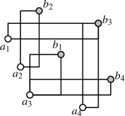
Figure 2: A BRF $\mathcal{R}(A,B)$ with a non-integral independent set polytope. The point $x\in\mathbb{R}^{\mathcal{R}}$ satisfying $x_{R}=1/2$ for the five rectangles shown, and $x_{R}=0$ for every other rectangle, is a vertex with non-integral coordinates.

Nevertheless, we will prove that the linear program obtained when we optimize on the all-ones direction:

$$\mathbf{mis}_{\mathrm{LP}}(\mathcal{R}) =\max\bigg{\{}\sum_{R\in\mathcal{R}}x_{R}:x\in\textrm{QSTAB}(\mathcal{R})\bigg{\}},$$

has an optimal integral solution. Recalling that $\mathbf{mis}(\mathcal{R})$ is the integral version of $\mathbf{mis}_{\mathrm{LP}}(\mathcal{R})$, this result can be stated as follows:

Theorem 3.2.

Let $\mathcal{R}$ be a non-empty BRF. There is an optimal integral solution for $\mathbf{mis}_{\mathrm{LP}}(\mathcal{R})$. In other words, $\mathbf{mis}_{\mathrm{LP}}(\mathcal{R})=\mathbf{mis}(\mathcal{R})$.

To prove Theorem 3.2, we look at optimal solutions for $\mathbf{mis}_{\mathrm{LP}}(\mathcal{R})$ minimizing the geometric area. More precisely, we consider the modified linear program $\overline{\mathbf{mis}}_{\mathrm{LP}}(\mathcal{R})$, where $\mathrm{area}(R)$ denotes the geometric area of a rectangle $R\in\mathcal{R}$ and $z^{*}$ denotes the optimal cost of $\mathbf{mis}_{\mathrm{LP}}(\mathcal{R})$:

$$\overline{\mathbf{mis}}_{\mathrm{LP}}(\mathcal{R}) =\min\bigg{\{}\sum_{R\in\mathcal{R}}\mathrm{area}(R)x_{R}:\sum_{R\in\mathcal{R}}x_{R}=z^{*};x\in\textrm{QSTAB}(\mathcal{R})\bigg{\}}\enspace.$$

Here we are using the function $\mathrm{area}\colon\mathcal{R}\to\mathbb{R}$, given by $\mathrm{area}([a_{x},b_{x}]\times[a_{y},b_{y}])=(b_{x}-a_{x})\cdot(b_{y}-a_{y})$, but the argument that follows works for any function satisfying (1) Nonnegativity: $\mathrm{area}(R)\geq 0$, (2) Strict monotonicity: If $R\subset S$, then $\mathrm{area}(R)<\mathrm{area}(S)$, and (3) Crossing bisubmodularity: If $R=I\times J$, $S=I^{\prime}\times J^{\prime}$ are two corner-intersecting rectangles in $\mathcal{R}_{\downarrow}$ then $\mathrm{area}((I\cup I^{\prime})\times(J\cap J^{\prime}))+\mathrm{area}((I\cap I^{\prime})\times(J\cup J^{\prime}))<\mathrm{area}(R)+\mathrm{area}(S)$.

Let $x^{*}$ be an arbitrary optimal extreme point of $\overline{\mathbf{mis}}_{\mathrm{LP}}(\mathcal{R})$ and let $\mathcal{R}_{0}=\{R\in\mathcal{R}:x^{*}_{R}>0\}$ be the support of $x^{*}$. Since $x^{*}$ minimizes weighted area, $\mathcal{R}_{0}$ is a subset of the collection of inclusion-wise minimal rectangles $\mathcal{R}_{\downarrow}$.

By Lemma 2.2, the only type of corner-intersection that can occur in $\mathcal{R}_{\downarrow}$ is the one depicted in Figure 3 (a). Next, we prove that those intersections never arise in $\mathcal{R}_{0}$.

Proposition 3.3.

The family $\mathcal{R}_{0}$ is c.f.i.

Proof.

Suppose that $R=\Gamma(a,b)$ and $R^{\prime}=\Gamma(a^{\prime},b^{\prime})$ are rectangles in $\mathcal{R}_{0}$ with corner-intersection as in Figure 3 (a).

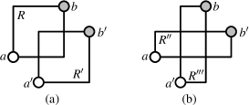
Figure 3: Proof of Proposition 3.3.

In Figure 3 (b) we show two rectangles, $R^{\prime\prime}=\Gamma(a,b^{\prime})$ and $R^{\prime\prime\prime}=\Gamma(a^{\prime},b)$, that also belong to $\mathcal{R}_{\downarrow}$. We modify $x^{*}$, first reducing the values of $x^{*}_{R}$ and $x^{*}_{R^{\prime}}$ by $\lambda\equiv\min\{x^{*}_{R},x^{*}_{R^{\prime}}\}$ and then increasing the values of $x^{*}_{R^{\prime\prime}}$ and $x^{*}_{R^{\prime\prime\prime}}$ by $\lambda$. Let $\bar{x}^{*}$ be this modified solution.

Since the weight of the rectangles covering any point in the plane can only decrease (that is, $\sum_{S\ni q}x^{*}_{S}\geq\sum_{S\ni q}\bar{x}^{*}_{S},\forall q\in[n]^{2}$), all the constraints $\sum_{S\ni q}\bar{x}^{*}_{S}\leq 1$ must hold. We also have $\sum_{S\in\mathcal{R}}\bar{x}^{*}_{S}=\sum_{S\in\mathcal{R}}x^{*}_{S}=z^{*}$, and therefore $\bar{x}^{*}$ is a feasible solution for $\overline{\mathbf{mis}}_{\mathrm{LP}}(\mathcal{R})$. But the total weighted area of $\bar{x}^{*}$ is $\lambda\left((\mathrm{area}(R)+\mathrm{area}(R^{\prime}))-(\mathrm{area}(R^{\prime\prime})+\mathrm{area}(R^{\prime\prime\prime})\right)>0$ units smaller than the one of the original solution $x^{*}$, contradicting its optimality. ∎

The fact that the support of $x^{*}$ forms a corner-free intersection family is all we need to prove the integrality of $x^{*}$:

Proposition 3.4.

The point $x^{*}$ is integral. In particular, $\mathcal{R}_{0}$ is a maximum independent set of $\mathcal{R}$.

Proof.

Since $\mathcal{R}_{0}$ is the support of $x^{*}$, the linear program $\mathbf{mis}_{\mathrm{LP}}(\mathcal{R}_{0})$ also has $x^{*}$ as optimal solution. But $\mathcal{I}(\mathcal{R}_{0})$ is a comparability graph by Proposition 2.1; therefore, $\textrm{QSTAB}(\mathcal{R}_{0})$ is integral. To conclude, we show that $x^{*}$ is an extreme point of $\textrm{QSTAB}(\mathcal{R}_{0})$. Indeed, if this does not hold, then $x^{*}$ can be written as convex combination of two points in $\textrm{QSTAB}(\mathcal{R}_{0})\subseteq\textrm{QSTAB}(\mathcal{R})$, contradicting the fact that $x^{*}$ is extreme of $\textrm{QSTAB}(\mathcal{R})$. ∎

The previous proposition concludes the proof of Theorem 3.2. Furthermore, since $\textrm{QSTAB}(\mathcal{R})$ has polynomially many variables and constraints, we obtain the following algorithmic result.

Theorem 3.5.

We can compute a MIS of a BRF in polynomial time.

4 A combinatorial algorithm for MIS and MHS of a BRF

In this section we devise an algorithm that constructs a maximum independent set $I^{*}$ and a minimum hitting set $H^{*}$ of a given BRF $\mathcal{R}(A,B,\mathcal{Z})$. The overall description of our algorithm is as follows. We first construct the family $\mathcal{R}_{\downarrow}$ of inclusionwise minimal rectangles of $\mathcal{R}$. Using a greedy procedure, we then find a maximal c.f.i. family of rectangles $\mathcal{K}\subseteq\mathcal{R}_{\downarrow}$. Next, we use Lemma 2.4 to construct an independent set $I^{*}$ and a hitting set $H_{0}$ of the same size for the family $\mathcal{K}$. Afterwards, we use a flipping procedure to transform $H_{0}$ into a set $H^{*}$ of the same cardinality in such a way that $H^{*}$ is also a hitting set for $\mathcal{R}_{\downarrow}$, and therefore for $\mathcal{R}$. Since $I^{*}$ and $H^{*}$ have the same cardinality, they are both optimal.

The following notation will be useful to describe our algorithm. Given a rectangle $R$, let $\mathbf{A}(R)$, $\mathbf{B}(R)$, $\mathbf{C}(R)$ and $\mathbf{D}(R)$ be the bottom-left corner, top-right corner, top-left corner and bottom-right corners of $R$, respectively. The notation is chosen so that if $R$ is a rectangle of the BRF $\mathcal{R}(A,B,\mathcal{Z})$, then $\mathbf{A}(R)\in A$ and $\mathbf{B}(R)\in B$ are the two defining corners of $R$.

Let $\mathcal{R}_{\downarrow}$ be the set of inclusion-wise minimal rectangles of $\mathcal{R}$. The construction of the c.f.i. family $\mathcal{K}$ uses a specific order in $\mathcal{R}_{\downarrow}$: We say that a rectangle $R$ precedes a rectangle $S$ in right-top order if the top-left corner of $R$ is lexicographically smaller than the top-left corner of $S$, this is,

• $\mathbf{C}(R)_{x}<\mathbf{C}(S)_{x}$, or

• $\mathbf{C}(R)_{x}=\mathbf{C}(S)_{x}$ and $\mathbf{C}(R)_{y}<\mathbf{C}(S)_{y}$ .

Let $R_{1},R_{2},\ldots,R_{t}$ be the rectangles in $\mathcal{R}_{\downarrow}$ sorted in right-top order. Observe that the top-left corners of these rectangles are sorted from left to right and, in case of ties, from bottom to top, hence the notation right-top order. In Figure 4 there is an example of rectangles sorted in this way.

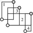
Figure 4: Some rectangles labeled in right-top order.

To construct $\mathcal{K}$, we process the rectangles in the sequence $(R_{i})_{i=1}^{t}$ one by one. The rectangle $R_{i}$ being processed is added to $\mathcal{K}$ if its addition keeps $\mathcal{K}$ corner-free. The set $\mathcal{K}$ obtained by this simple greedy procedure is a maximal c.f.i. subfamily of $\mathcal{R}_{\downarrow}$. As stated before, we then use Lemma 2.4 to compute a maximum independent set $I^{*}$ and a minimum hitting set $H_{0}$ for $\mathcal{K}$. As we will prove later, $I^{*}$ is actually a maximum independent set of the entire family $\mathcal{R}$. We can further assume that the points in $H_{0}$ have integral coordinates in $[n]^{2}$, because every rectangle hit by $(p_{x},p_{y})$ is also hit by $(\left\lceil p_{x}\right\rceil,\left\lceil p_{y}\right\rceil)$.

The last step of the algorithm consists of a flipping procedure that essentially moves the points of $H_{0}$ around so that, in their new position, they not only hit $\mathcal{K}$ but the entire family $\mathcal{R}$. As we discuss in Section 6, the underlying ideas for this flipping algorithm are already present in Frank’s algorithmic proof of Gy$\ddot{\mathrm{o}}$ri’s min-max result on intervals [28].

Consider a set $H\subseteq\mathbb{Z}^{2}$ and two points $p,q\in H$ with $p_{x}<q_{x}$, and $p_{y}<q_{y}$. By flipping $p$ and $q$ in $H$ we mean to move these two points to the new coordinates $r=(p_{x},q_{y})$ and $s=(q_{x},p_{y})$. More precisely, this means replacing $H$ by $H^{\prime}=H\setminus\{p,q\}\cup\{r,s\}$. The following lemma states that flipping points of $H$ that are inside a rectangle of $\mathcal{R}_{\downarrow}$ can only increase the family of rectangles of $\mathcal{R}_{\downarrow}$ that are hit by $H$.

Lemma 4.1.

Let $R$ be a rectangle in $\mathcal{R}_{\downarrow}$ that contains $p$ and $q$. If $S\in\mathcal{R}_{\downarrow}$ is hit by $H$ then it is also hit by $H^{\prime}=H\setminus\{p,q\}\cup\{r,s\}$.

Proof.

Assume by contradiction that $S$ is hit by $H$ but not by $H^{\prime}$. Assume also that $S$ is hit by $p$ (the case where $S$ is hit by $q$ is analogous). Since $S$ does not contain $r$ nor $s$, the point $b=\mathbf{B}(S)$ must be in the region $[p_{x},q_{x}-1]\times[p_{y},q_{y}-1]$. In particular, $b\in R\setminus\{\mathbf{A}(R),\mathbf{B}(R)\}$. By Lemma 2.2, this contradicts the inclusion-wise minimality of $R$. ∎

We can now describe the flipping procedure. Let $K_{1},\ldots,K_{k}$ be the sequence of rectangles in $\mathcal{K}$ in right-top order, and $H$ be a set initially equal to $H_{0}$. In the $j$-th iteration of this procedure, we find the point $p$ in $H\cap K_{j}$ of minimum $y$-coordinate and the point $q$ in $H\cap K_{j}$ of maximum $x$-coordinate (breaking ties arbitrarily). Since we maintain $H$ as a hitting set for $\mathcal{K}$, both points $p$ and $q$ exist. We then check if both points can be flipped (i.e. if $p_{x}<q_{x}$ and $p_{y}<q_{y}$) and in that case, we update $H$ by flipping $p$ and $q$. The description of our entire algorithm is depicted as Algorithm 1.

Algorithm 1 for MIS and MHS of a BRF $\mathcal{R}(A,B,\mathcal{Z})$.

1:Construct $\mathcal{R}_{\downarrow}$ and sort them as $(R_{i})_{i=1}^{t}$ in right-top order.

2:Greedily construct a maximum c.f.i. family $\mathcal{K}$ from the sequence $(R_{i})_{i=1}^{t}$. Let $(K_{j})_{j=1}^{k}$ be the family $\mathcal{K}$ sorted in right-top order.

3:Find a maximum independent set $I^{*}$ and a minimum hitting set $H$ for $\mathcal{K}$.

4:for $j=1$ to $k$ do $\triangleright$ Flipping procedure starts.

5:     Let $p$ be a point of minimum $y$-coordinate in $H\cap K_{j}$ and $q$ be a point of maximum $x$-coordinate in $H\cap K_{j}$.

6:     if $p_{x}<q_{x}$ and $p_{y}<q_{y}$ then

7:         $H\leftarrow H\setminus\{p,q\}\cup\{(p_{x},q_{y}),(q_{x},p_{y})\}$ $\triangleright$ Flip $p$ and $q$ in $H$.

8:     end if

9:end for

10:Return $I^{*}$ and $H^{*}\leftarrow H$.

To analyze the correctness of Algorithm 1 we need an auxiliary definition. Recall that if a rectangle $R_{i}$ in the sorted sequence $\mathcal{R}_{\downarrow}$ is not included in $\mathcal{K}$ then $R_{i}$ must have corner-intersection with a rectangle $R_{i^{\prime}}\in\mathcal{K}$ with $i^{\prime}<i$. The rectangle $R_{i^{\prime}}\in\mathcal{K}$ with largest index that has corner-intersection with $R_{i}$ is denoted as the witness of $R_{i}$, and written as $R_{i^{\prime}}=\mathrm{wit}(R_{i})$. By Lemma 2.2, the fact that $\mathrm{wit}(R_{i})$ precedes $R_{i}$ in right-top order implies that $\mathbf{D}(\mathrm{wit}(R_{i}))\in\mathrm{int}(R_{i})$ and $\mathbf{C}(R_{i})\in\mathrm{int}(\mathrm{wit}(R_{i}))$.

Lemma 4.2.

After iteration $j$ of the flipping procedure, the set $H$ hits every rectangle in $\mathcal{K}$ and every rectangle in $\mathcal{R}_{\downarrow}\setminus\mathcal{K}$ with witness in $\{K_{l}\colon l\leq j\}$.

Proof.

Observe that the algorithm only flips pairs of points that are inside a given rectangle $K_{j}$ of $\mathcal{R}_{\downarrow}$. By Lemma 4.1, the collection of rectangles hit by $H$ increases in every iteration. So we only need to prove that after iteration $j$ all the rectangles witnessed by $K_{j}$ are hit. We do this by induction.

If every rectangle witnessed by $K_{j}$ is hit at the end of iteration $j-1$, we are done. Suppose then, that at then end of iteration $j-1$ there is at least one rectangle $R$ in $\mathcal{R}_{\downarrow}\setminus\mathcal{K}$ witnessed by $K_{j}$ that has not been hit. Let $a=\mathbf{A}(K_{j}),b=\mathbf{B}(K_{j}),a^{\prime}=\mathbf{A}(R)$ and $b^{\prime}=\mathbf{B}(R)$ so that $K_{j}=\Gamma(a,b)$ and $R=\Gamma(a^{\prime},b^{\prime})$. Since $K_{j}$ precedes $R$ in right-top order and they have corner-intersection, the relative position of both rectangles must be as depicted in Figure 5.

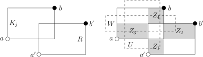
Figure 5: On the left, the two rectangles $K_{j}=\Gamma(a,b)$ and $R=\Gamma(a^{\prime},b^{\prime})$ with $\mathrm{wit}(R)=K_{j}$. On the right, auxiliary constructions for the proof of Lemma 4.2

Observe that the rectangles $S=\Gamma(a^{\prime},b)$ and $T=\Gamma(a,b^{\prime})$ are in $\mathcal{R}_{\downarrow}$. We claim that $S\in\mathcal{K}$ and that $T$ is already hit by $H$.

Let us prove the first claim. Assume this is not the case; then $S\in\mathcal{R}_{\downarrow}\setminus\mathcal{K}$ must have a witness $U=\mathrm{wit}(S)$ in $\mathcal{K}$. Let $d=\mathbf{D}(U)$ be the bottom-right corner of $U$. Since $S$ and $U$ have corner-intersection and $U$ precedes $S$, the point $d$ is in the interior of $S$. Furthermore, since $U$ and $K_{j}$ are both in $\mathcal{K}$, $d$ cannot be in the interior of $K_{j}$. We conclude that $d\in Z_{1}:=\mathrm{int}(S)\setminus\mathrm{int}(K_{j})=(a^{\prime}_{x},b_{x})\times(a^{\prime}_{y},a_{y}]$. See Figure 5 for reference. But since $U$ contains the top-left corner of $S$ in its interior (because $U$ and $S$ have corner-intersection) and $U$ does not contain $a$ on its interior (as otherwise $U$ would not be inclusionwise minimal), we conclude that $K_{j}$ precedes $U$ in right-top order. But then, $U$ is a rectangle in $\mathcal{K}$ having corner-intersection with $R$ and appearing after $K_{j}$ in right-top order. This contradicts the definition of $K_{j}$ as witness of $R$, and concludes the proof of the first claim.

Let us prove the second claim. If $T=\Gamma(a,b^{\prime})$ is in $\mathcal{K}$ then we are done as $H$ is a hitting set for $\mathcal{K}$. So assume that $T\in\mathcal{R}_{\downarrow}\setminus\mathcal{K}$. Let $W=\mathrm{wit}(T)$ and $d^{\prime}=\mathbf{D}(W)$. Since $W$ and $T$ have corner-intersection and $W$ precedes $T$, $d^{\prime}$ is in the interior of $T$. Furthermore, since both $W$ and $K_{j}$ are in $\mathcal{K}$, $d^{\prime}$ is not in the interior of $K_{j}$. We conclude that $d^{\prime}\in Z_{2}:=\mathrm{int}(T)\setminus\mathrm{int}(K_{j})=[b_{x},b^{\prime}_{x})\times(a_{y},b^{\prime}_{y})$. Since $W$ contains the top-left corner of $T$ in its interior (because $W$ and $T$ have corner-intersection), we deduce that $W$ precedes $K_{j}$ in right-top order. But then $W=K_{j^{\prime}}$ for $j^{\prime}<j$ and so, by induction hypothesis, rectangle $T$ was hit at the end of iteration $j^{\prime}$. This concludes the proof of the second claim.

Recall that $R$ is not hit by $H$ at the end of iteration $j-1$. Since $T$ is hit by $H$ the set $H\cap T\setminus R$ must be nonempty. In particular, the point $p$ chosen by the algorithm, of minimum $y$-coordinate in $K_{j}\cap H$ must be in the zone $Z_{3}:=[a_{x},a^{\prime}_{x})\times[a_{y},b^{\prime}_{y}]$. Similarly, since $S\in\mathcal{K}$, it must be hit by $H$ and so the set $H\cap S\setminus R$ is nonempty. Therefore, the point $q$ chosen by the algorithm of maximum $x$-coordinate in $K_{j}\cap H$ is in the zone $Z_{4}:=[a^{\prime}_{x},b_{x}]\times(b^{\prime}_{y},b_{y}]$. In particular, $p_{x}<q_{x}$, $p_{y}<q_{y}$ and the point $s=(q_{x},p_{y})$ is in $R$. We conclude that after flipping $p$ and $q$ in $H$, the rectangle $R$ is hit. ∎

Thanks to the previous lemma we obtain our main combinatorial result.

Theorem 4.3.

Algorithm 1 returns an independent set $I^{*}$ and a hitting set $H^{*}$ of $\mathcal{R}(A,B,\mathcal{Z})$ of the same cardinality. In particular, they are both optimal and $\mathbf{mis}(\mathcal{R})=\mathbf{mhs}(\mathcal{R})$.

Proof.

The fact that $I^{*}$ is an independent set of $\mathcal{R}$ follows by construction and the fact that $\mathcal{K}\subseteq\mathcal{R}$. By Lemma 4.2, the set $H^{*}$ returned by the algorithm hits all the elements in $\mathcal{R}_{\downarrow}$. Since every rectangle in $\mathcal{R}$ contains a rectangle in $\mathcal{R}_{\downarrow}$, $H^{*}$ is also a hitting set of $\mathcal{R}$. Finally, since $H^{*}$ was constructed from $H_{0}$ via a sequence of flips which preserve cardinality and since $|H_{0}|=|I^{*}|$ by Lemma 2.3, we obtain that $|I^{*}|=|H^{*}|$. As every hitting set has cardinality as least as large as every independent set, we conclude that both are optimal. ∎

It is quite simple to give a polynomial time implementation of Algorithm 1. In Subsection 4.1, we discuss an efficient implementation that runs in $O(\operatorname{matching}(n\log n,n^{2})+n^{2}\log^{2}n)$ time, where $n=|A\cup B|$. Here we are assuming that testing containment in $\mathcal{Z}$ can be done in unit time. Otherwise, we need additional $O(n^{2}T(\mathcal{Z}))$ time, where $T(\mathcal{Z})$ is the time for testing containment in $\mathcal{Z}$.

4.1 Implementation of the combinatorial algorithm

To implement our algorithm it will be useful to have access to a data structure for dynamic orthogonal range queries. That is, a structure to store a dynamic collection of points $P$ in the plane, supporting insertions, deletions and queries of the following type: given an axis-parallel rectangle $Q$, is there a point $p$ in $Q\cap P$? And if there is one, report any.

There are many data structures we can use. For our purposes, it would be enough to use any structure in which each operation takes polylogarithmic (or even subpolynomial) time. For concreteness, we use the following result of Willard and Lueker [55], specialized to two-dimensional Euclidean space.

Theorem 4.4 ((Willard and Lueker)).

There is a point data structure for orthogonal range queries in the plane on $n$ points supporting insertion, deletion and queries in time $O(\log^{2}n)$, and using space $O(n\log n)$.

Using this data structure, we can easily implement Algorithm 1. Indeed, let us first see how to construct $\mathcal{R}_{\downarrow}$.

Start by inserting the points in $A$ and $B$ to the point data structure and creating an empty list $\mathcal{R}_{\downarrow}$. For each point $a$ in $A$ sorted from left to right and each point $b$ in $B$ from bottom to top check if $\Gamma(a,b)$ is a rectangle in $\mathcal{R}$ (i.e., if $a\leq_{\mathbb{R}^{2}}b$ and if $\Gamma(a,b)\subseteq\mathcal{Z}$) and if it has no points of $A\cup B$ in its interior using the data structure. If both conditions hold, add $\Gamma(a,b)$ to the end of $\mathcal{R}_{\downarrow}$. Note that by going through $A\times B$ in this order, the list $\mathcal{R}_{\downarrow}$ is sorted in right-top order. It is easy to see that the entire procedure takes time $O(n^{2}\log^{2}n+n^{2}T(\mathcal{Z}))$.

Constructing $\mathcal{K}$ is similar. Start by creating an empty list $\mathcal{K}$ and a point data structure $\mathbf{D}$ containing the bottom-right corners of all rectangles in $\mathcal{R}_{\downarrow}$. Then, go through the ordered list $\mathcal{R}_{\downarrow}$ once again and add the current rectangle $R\in\mathcal{R}_{\downarrow}$ to the end of $\mathcal{K}$ if $R$ does not contain a point of $\mathbf{D}$ in its interior. It is easy to see that we obtain the sorted c.f.i. family $\mathcal{K}$ described in our algorithm in this way and that the entire procedure takes time $O(|\mathcal{R}_{\downarrow}|\log^{2}(|\mathcal{K}|))=O(n^{2}\log^{2}(|\mathcal{K}|))$.

Afterwards, construct the intersection graph $\mathcal{I}(\mathcal{K})$ in $O(|\mathcal{K}^{2}|)$ time and then use Lemma 2.4 to get a maximum independent set $I^{*}$ and a minimum hitting set $H_{0}$ of $\mathcal{K}$ in time $O(\operatorname{matching}(|\mathcal{K}|,|E(I(\mathcal{K}))|)$.

To implement the flipping procedure, we initialize a point data structure containing $H$ at every moment. Note that $|H|\leq n$ as $A\cup B$ is itself a hitting set of $\mathcal{R}$. In each of the $|\mathcal{K}|$ iterations of the flipping procedure we need to find the lowest point and the rightmost point of a range query. This can be done using binary search and the query operation of the data structure losing an extra logarithmic factor, i.e., in time $O(\log^{3}n)$. To flip two points of $H$, we perform two deletions and two insertions in time $O(\log^{2}n)$. The entire flipping procedure takes time $O(|\mathcal{K}|\log^{3}n)$.

In Subsection 4.2 we prove that $|\mathcal{K}|=O(n\log n)$ and $|E(\mathcal{I}(\mathcal{K}))|=O(n^{2})$. By using these bounds and the previous discussion, we conclude that Algorithm 1 can be implemented to run in time $O(\operatorname{matching}(n\log n,n^{2})+n^{2}\log^{2}n+n^{2}T(\mathcal{Z})).$

Hopcroft and Karp’s [35] algorithm for maximum matching on a bipartite graph with $v$ vertices and $e$ edges runs in time $O(e\sqrt{v})$. Specializing this to $v=O(n\log n)$ and $e=O(n^{2})$, $\operatorname{matching}(n\log n,n^{2})$ is time $O(n^{2.5}\sqrt{\log n})$. On the other hand, Mucha and Sankowski [42] have devised a randomized algorithm that returns with high probability a maximum matching of a bipartite graph in time $O(v^{\omega})$, where $\omega$ is the exponent for square matrix multiplication. The current best upper bound for $\omega$ is approximately $2.3727$ by Williams [56]. From this discussion, we obtain the following result.

Theorem 4.5.

We can implement Algorithm 1 to run in time

$$O\left(\operatorname{matching}(n\log n,n^{2})+n^{2}\log^{2}n+n^{2}T(\mathcal{Z})\right),$$

where $n=|A\cup B|$ and $T(\mathcal{Z})$ is the time needed to test if a rectangle is contained in $\mathcal{Z}$. Using Hopcroft and Karp’s implementation, this is

$$O(n^{2.5}\sqrt{\log n}+n^{2}T(\mathcal{Z})).$$

Using Mucha and Sankowski’s randomized algorithm, the running time can be reduced to

$$O((n\log n)^{\omega}+n^{2}T(\mathcal{Z})),$$

where $\omega<2.3727$ is the exponent for square matrix multiplication.

4.2 Bounds for $\mathcal{K}$.

The bounds we prove on this section are valid for every corner-free intersection subfamily of $\mathcal{R}_{\downarrow}$. Given one such family $\mathcal{K}$, define its lower-left corner set $\mathbf{A}(\mathcal{K})=\{\mathbf{A}(K)\colon K\in\mathcal{K}\}$ and its upper-right corner set $\mathbf{B}(\mathcal{K})=\{\mathbf{A}(K)\colon K\in\mathcal{K}\}$. We start with a simple result.

Lemma 4.6.

If all the rectangles of $\mathcal{K}$ intersect a fixed vertical (or horizontal) line $\lambda$, then $|\mathcal{K}|\leq\lvert\mathbf{A}(\mathcal{K})\rvert+\lvert\mathbf{B}(\mathcal{K})\rvert-1.$

Proof.

Project all the rectangles in $\mathcal{K}$ onto the line $\lambda$ to obtain a collection of intervals in the line. Since $\mathcal{K}$ is a c.f.i. family, the collection of intervals forms a laminar family: if two intervals intersect, then one is contained in the other. Let $X$ be the collection of extreme points of the intervals. Since by assumption no two points in $A\cup B$ share coordinates, $|X|=\lvert\mathbf{A}(\mathcal{K})\rvert+\lvert\mathbf{B}(\mathcal{K})\rvert$ and furthermore, every interval is a non-singleton interval. To conclude the proof of the lemma we use the following known fact, which can be proved by induction: every laminar family of non-singleton intervals with extreme points in $X$ has cardinality at most $\lvert X\rvert-1$. ∎

Now we consider the situation where the family $\mathcal{K}$ is not necessarily stabbed by a single line.

Lemma 4.7.

Let $\mathcal{L}=\{\lambda_{1},\ldots,\lambda_{r}\}$ be a collection of vertical lines that intersect all the rectangles in $\mathcal{K}$, then $|\mathcal{K}|\leq n(1+\lfloor\log_{2}(r)\rfloor)-r.$

Proof.

Assume that $\lambda_{1},\ldots,\lambda_{r}$ is sorted from left to right. Consider the following collections of vertical lines:

$$\mathcal{L}_{0} =\{\lambda_{2k+1}\colon k\geq 0\}=\{\lambda_{1},\lambda_{3},\lambda_{5},\lambda_{7},\lambda_{9}\ldots\}.$$

$$\mathcal{L}_{1} =\{\lambda_{4k+2}\colon k\geq 0\}=\{\lambda_{2},\lambda_{6},\lambda_{10},\lambda_{14},\ldots\}.$$

$$\mathcal{L}_{2} =\{\lambda_{8k+4}\colon k\geq 0\}=\{\lambda_{4},\lambda_{12},\lambda_{20},\lambda_{28},\ldots\}.$$

$$\cdots$$

$$\mathcal{L}_{t} =\{\lambda_{2^{t}(2k+1)}\colon k\geq 0\}.$$

The collections $\mathcal{L}_{0},\dots,\mathcal{L}_{\lfloor\log_{2}(r)\rfloor}$ form a partition of $\mathcal{L}$. Include each rectangle $R$ in $\mathcal{K}$ into the set $\mathcal{K}_{t}$, $0\leq t\leq\lfloor\log_{2}(r)\rfloor$, of largest index such that $\mathcal{L}_{t}$ contains a vertical line that intersects $R$. See Figure 6 for an example illustrating this construction.

Figure 6: The dotted lines, thin lines and thick lines correspond to $\mathcal{L}_{0}$, $\mathcal{L}_{1}$ and $\mathcal{L}_{2}$ respectively. White, light-gray and dark-gray rectangles are assigned to $\mathcal{K}_{0}$, $\mathcal{K}_{1}$ and $\mathcal{K}_{2}$ respectively.

Fix an index $t$. Every rectangle in $\mathcal{K}_{t}$ intersect a unique line in $\mathcal{L}_{t}$ (if it intersects two or more, then it would also intersect a line in $\mathcal{L}_{t+1}$). For a given line $\lambda\in\mathcal{L}_{t}$, let $\mathcal{K}_{\lambda}$ be the family of rectangles in $\mathcal{K}_{t}$ intersecting $\lambda$. By Lemma 4.6, the number of rectangles in $\mathcal{K}_{\lambda}$ is at most $\lvert\mathbf{A}(\mathcal{K}_{\lambda})\rvert+\lvert\mathbf{B}(\mathcal{K}_{\lambda})\rvert-1$. Every point $a$ in $\mathbf{A}(\mathcal{K})$ belongs to exactly one set in $\{\mathbf{A}(\mathcal{K}_{\lambda}):\lambda\in\mathcal{L}_{t}\}$. It belongs to the one corresponding to the first line $\lambda$ is the first line on or to the right of $a$. Therefore, $\sum_{\lambda\in\mathcal{L}_{t}}\lvert\mathbf{A}(\mathcal{K}_{\lambda})\rvert\leq\lvert A\rvert$, and similarly, $\sum_{\lambda\in\mathcal{L}_{t}}\lvert\mathbf{B}(\mathcal{K}_{\lambda})\rvert\leq\lvert B\rvert$. Altogether we get $\lvert\mathcal{K}_{t}\rvert=\sum_{\lambda\in\mathcal{L}_{t}}\lvert\mathcal{K}_{\lambda}\rvert\leq\lvert\mathbf{A}(\mathcal{K})\rvert+\lvert\mathbf{B}(\mathcal{K})\rvert-\lvert\mathcal{L}_{t}\rvert\leq\lvert\mathbf{A}(\mathcal{K})\rvert+\lvert\mathbf{B}(\mathcal{K})\rvert$. Summing over $t$ we obtain $\lvert\mathcal{K}\rvert=\sum_{t=0}^{\lfloor\log_{2}(r)\rfloor}\lvert\mathcal{K}_{\lambda}\rvert\leq(1+\lfloor\log_{2}(r)\rfloor)(\lvert\mathbf{A}(\mathcal{K})\rvert+\lvert\mathbf{B}(\mathcal{K})\rvert)$.∎

If $\mathcal{K}$ is the c.f.i. family obtained with Algorithm 1, then $n$ vertical lines are enough to intersect all rectangles in $\mathcal{K}$. Therefore, $|\mathcal{K}|=O(n\log n)$. Let us now bound the number of edges of the intersection graph $\mathcal{I}(\mathcal{K})$.

Lemma 4.8.

$|E(\mathcal{I}(\mathcal{K}))|=O(n^{2}).$

Proof.

Let $\ell=|E(\mathcal{I}(\mathcal{K}))|$. Let also $\Lambda(n)$ be the maximum possible value of $\ell$ as a function of $n$. Recall that the vertices of all rectangles in $\mathcal{K}$ are in the grid $[n]^{2}$. Consider the vertical line $\lambda=\{(x,\lfloor n/2\rfloor)\colon x\in\mathbb{R}\}$ that divides the grid in two roughly equal parts. Count the edges in $\mathcal{I}(\mathcal{K})$ as follows. Let $E_{1}$ be the edges connecting pairs of rectangles that are totally to the left of $\lambda$, $E_{2}$ be the edges connecting pairs of rectangles that are totally to the right of $\lambda$, and $E_{3}$ be the remaining edges. We trivially get that $|E_{1}|\leq\Lambda(\lfloor n/2\rfloor)$ and $|E_{2}|\leq\Lambda(\lceil n/2\rceil)$. We bound the value of $|E_{3}|$ in a different way.

Let $\mathcal{K}_{\lambda}$ be the rectangles intersecting the vertical line $\lambda$. Then, $E_{3}$ is exactly the collection of edges in $\mathcal{I}(\mathcal{K})$ having an endpoint in $\mathcal{K}_{\lambda}$. By Lemma 4.6, $\lvert\mathcal{K}_{\lambda}\rvert\leq n$. Now we bound the degree of each element of $\mathcal{K}_{\lambda}$ in $\mathcal{I}(\mathcal{K})$. Consider one rectangle $R=\Gamma(a,b)\in\mathcal{K}_{\lambda}$. Every rectangle intersecting $R$ must intersect one of the four lines defined by its sides. By using again Lemma 4.6, we conclude that the degree of $R$ in $\mathcal{I}(\mathcal{K})$ is at most $4n$. Therefore, the number of edges having an endpoint in $\mathcal{K}_{\lambda}$ is at most $4n^{2}$.

We conclude that $\Lambda(n)$ satisfies the recurrence $\Lambda(n)\leq\Lambda(\lfloor n/2\rfloor)+\Lambda(\lceil n/2\rceil)+4n^{2},$ from which, $\Lambda(n)=O(n^{2})$.∎

To finish this section, we note that it is is very easy to construct a family $\mathcal{K}$, for which $|E(\mathcal{I}(\mathcal{K}))|=\Omega(n^{2})$. See Figure 7 for an example. In this example, $\mathcal{K}$ was obtained using the greedy procedure. Also, if we let $n^{\prime}=|A|=|B|=n/2$, then $|\mathcal{K}|=2n^{\prime}+2$ and $|E(\mathcal{I}(\mathcal{K}))|=(n^{\prime})^{2}+4=\Omega(n^{2})$.

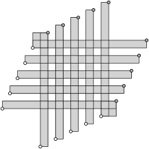
Figure 7: Example with $|E(\mathcal{I}(\mathcal{K}))|=\Omega(n^{2})$.

On the other hand, it is not clear if there are examples achieving $\lvert\mathcal{K}\rvert=\Omega(n\log n)$. In particular, we give the following conjecture

Conjecture 4.9.

For any c.f.i. family $\mathcal{K}$ with vertices in $[n]^{2}$, $\lvert\mathcal{K}\rvert=O(n)$.

If this conjecture holds, it is easy to get better bounds for the running time of Algorithm 1.

5 WMIS of BRFs and maximum weight cross-free matching

We now consider the problem of finding a maximum weight independent set of the rectangles in a BRF $\mathcal{R}(A,B,\mathcal{Z})$ with weights $\{w_{R}\}_{R\in\mathcal{R}}$. This problem is significantly harder than the unweighted counterpart.

Theorem 5.1.

The maximum weight independent set problem is $\mathbf{NP}$-hard for unrestricted BRFs even for weights in $\{0,1\}$.

Proof.

We reduce from the maximum independent set of rectangles problem, which is $\mathbf{NP}$-hard even if the vertices of the rectangles are all distinct [27]. Given an instance $\mathcal{I}$ with the previous property, let $A$ (resp. $B$) be the set of lower-left (resp. upper-right) corners of rectangles in $\mathcal{I}$. Note that $\mathcal{I}\subseteq\mathcal{R}(A,B)$ so we can find a maximum independent set of $\mathcal{I}$ by finding a maximum weight independent set in $\mathcal{R}$, where we give unit weight to each rectangle $R\in\mathcal{I}$, and zero weight to every other rectangle. ∎

Despite this negative result, we can still provide efficient algorithms for some interesting subclasses of BRFs graphs $G=(A\cup B,\mathcal{R})$. Since independent sets of $\mathcal{R}$ are in one to one correspondence with cross-free matchings of $G$, the problem we are studying in this section is equivalent to finding a maximum weight cross-free matching of $G$.

5.1 A hierarchy of subclasses of BRFs

We recall the following definitions of a nested family of bipartite graph classes. We keep the notation $G=(A\cup B,\mathcal{R})$ since they are all BRF graphs.

A bipartite permutation graph (or bipartite 2-dimensional graph) is the comparability graph of a two dimensional partially ordered set of height 2, where $A$ is the set of minimal elements and $B$ is the complement of this set. For our purposes, a two dimensional partially ordered set is simply a collection of points in $\mathbb{Z}^{2}$ with the relation $p\leq_{\mathbb{Z}^{2}}q$ if $p_{x}\leq q_{x}$ and $p_{y}\leq q_{y}$.

A convex bipartite graph $G=(A\cup B,\mathcal{R})$ is a bipartite graph admitting a labeling $\{a_{1},\ldots,a_{k}\}$ of $A$ so that the neighborhood of each $b\in B$ is a set of consecutive elements of $A$. A biconvex graph is a convex bipartite graph for which there is also a labeling for $B=\{b_{1},\ldots,b_{l}\}$ so that the neighborhood of each $a\in A$ is consecutive in $B$.

In an interval bigraph, each vertex $v\in A\cup B$ is associated to a real closed interval $I_{v}$ (w.l.o.g. with integral extremes) so that $a\in A$ and $b\in B$ are adjacent if and only if $I_{a}\cap I_{b}\neq\emptyset$.

A two directional orthogonal ray graph (2dorg) is a bipartite graph on $A\cup B$ where each vertex $v$ is associated to a point $(v_{x},v_{y})\in\mathbb{Z}^{2}$, so that $a\in A$ and $b\in B$ are connected if and only the rays $[a_{x},\infty)\times\{a_{y}\}$ and $\{b_{x}\}\times(-\infty,b_{y}]$ intersect each other. Since this condition is equivalent to $\Gamma(a,b)\in\mathcal{R}(A,B)$, two directional orthogonal ray graphs are exactly the unrestricted BRFs graphs.

It is known that the following strict inclusions hold for these classes [9, 51]: bipartite permutation $\subset$ biconvex $\subset$ convex $\subset$ interval bigraph $\subset$ 2dorg. There are also polynomial time algorithms to recognize if a graph belongs to any of these classes [51, 53, 45]. On the other hand, the problem of recognizing general (restricted) BRF graphs is open.

We give a simple geometrical interpretation of some of the classes presented above as unrestricted BRFs. The equivalence between the definitions below and the ones above are simple so the proof of equivalence is omitted. Bipartite permutation graphs are simply the unrestricted BRF graphs $G=(A\cup B,\mathcal{R})$ where no two points in the same color class are comparable under $\leq_{\mathbb{R}^{2}}$. Let $L=\{(x,-x)\colon x\in\mathbb{Z}\}$ be the integer points of the diagonal line $y=-x$. Similarly, let $L^{+}=\{(x,y)\in\mathbb{Z}^{2}\colon y\geq-x\}$ and $L^{-}=\{(x,y)\in\mathbb{Z}^{2}\colon y\leq-x\}$ be the points weakly above and weakly below $L$. Convex bipartite graphs are those unrestricted BRF graphs $G=(A\cup B,\mathcal{R})$ where $A\subset L$ and $B\subset L^{+}$. Interval bigraphs are those unrestricted BRF graphs where $A\subset L^{-}$ and $B\subset L^{+}$.

In the following subsections we investigate the maximum weight cross-free matching problem on these subclasses.

5.2 Bipartite permutation graphs

Every bipartite permutation graph $G$ is the graph representation of a BRF $\mathcal{R}(A,B)$ such that no two points in the same color class ($A$ or $B$) are comparable under $\leq_{\mathbb{R}^{2}}$. In this case we say that $\mathcal{R}(A,B)$ is a bipartite permutation BRF and we can define a partial order $\searrow$ on its rectangles. We say that $R\searrow S$ if $R$ and $S$ are disjoint and at least one of $R_{x}<S_{x}$ and $R_{y}>S_{y}$ holds. It is not hard to verify (see, e.g., Brandstädt [8]) that $(\mathcal{R},\searrow)$ is a partial order whose comparability graph is the complement of $\mathcal{I}(\mathcal{R})$. In what follows, we use this fact to devise polynomial time algorithms for the maximum weight independent set of bipartite permutation BRFs.

Observe that $\mathcal{I}(\mathcal{R})$ is a perfect graph (because so is its complement [40]); therefore, using Proposition 3.1 we can compute a maximum weight independent set of $\mathcal{R}$ in polynomial time by finding an optimal vertex of

$$\mathbf{mis}_{\mathrm{LP}}(\mathcal{R},w) \equiv\max\bigg{\{}\sum_{R\in\mathcal{R}}w_{R}x_{R}\colon\sum_{R:\ q\in R}x_{R}\leq 1,\text{$q\in[n]^{2}$};x\geq 0\bigg{\}}\enspace.$$

We can also do this combinatorially using that the maximum weight independent sets in $\mathcal{R}$ are exactly the maximum weight chains on the weight partially ordered set $(\mathcal{R},\searrow)$.

Theorem 5.2.

There is an $O(n^{2})$ algorithm for the maximum weight cross-free matching (and hence, for WMIS) of bipartite permutation graphs.

Proof.

For simplicity, let us assume that all the weights are different. Our algorithm exploits the geometric structure of the independent sets in $\mathcal{R}$. Since $A$ and $B$ are antichains of $\leq_{\mathbb{R}^{2}}$, the condition $R\searrow S$ implies that $\mathbf{A}(R)_{x}<\mathbf{A}(S)_{x}$ and $\mathbf{B}(R)_{y}>\mathbf{B}(S)_{y}$. Let $\mathcal{R}^{*}\subset\mathcal{R}$ be any maximum weight independent set and let $R\searrow S\searrow T$ be three consecutive rectangles in $\mathcal{R}^{*}$. We can extract the following information about $S$ (see Figure 8 for the first two scenarios, the other two are analogous):

• Down-right scenario:
  If $R_{y}>S_{y}$ and $S_{x}<T_{x}$, then (i) $S$ is the heaviest rectangle with corner $\mathbf{B}(S)$. In particular, $S$ is determined by $\mathbf{B}(S)$.

• Down-down scenario:
  If $R_{y}>S_{y}$ and $S_{y}>T_{y}$, then (ii) $S$ is the heaviest rectangle below $R$ with corner $\mathbf{A}(S)$. In particular, $S$ is determined by $\mathbf{A}(R)_{y}$ and $\mathbf{A}(S)$.

• Right-down scenario:
  If $R_{x}<S_{x}$ and $S_{y}>T_{y}$, then (iii) $S$ is the heaviest rectangle with corner $\mathbf{A}(S)$. In particular, $S$ is determined by $\mathbf{A}(S)$.

• Right-right scenario:
  If $R_{x}<S_{x}$ and $S_{x}<T_{x}$, then (iv) $S$ is the heaviest rectangle to the right of $R$ with corner $\mathbf{B}(S)$. In particular, $S$ is determined by $\mathbf{B}(S)$ and $\mathbf{B}(R)_{x}$.

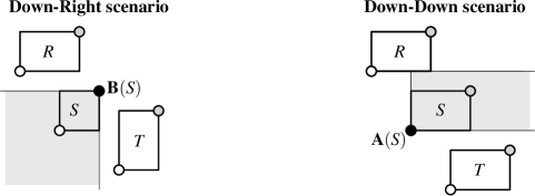
Figure 8: Proof of Theorem 5.2.

For $R\in\mathcal{R}$, let $V(R)$ be the maximum weight of a path in $(\cal{R},\searrow)$ that starts with $R$. For $a\in A$, let $V_{\downarrow}(a)$ be the maximum weight of a path using only rectangles below $a$. Similarly, for $b\in B$, let $V_{\rightarrow}(b)$ be the maximum weight of a path using only rectangles to the right of $b$.

Clearly, $V_{\downarrow}(a)=\max\left\{V(S)\colon\text{$S$ rectangle below $a$}\right\}$, but from the decomposition into scenarios we can restrict $S$ to be a rectangle below $a$ satisfying properties (i) or (ii). Using this idea, we define:

• $S(a)=$ the heaviest rectangle with $\mathbf{A}(S)=a$,

• $S(a,a^{\prime})=$ the heaviest rectangle below $a$ with $\mathbf{A}(S)=a^{\prime}$,

• $T(b)=$ the heaviest rectangle with $\mathbf{B}(S)=b$,

• $T(b,b^{\prime})=$ the heaviest rectangle to the right of $b$ with $\mathbf{B}(S)=b^{\prime}$,

• $\mathcal{S}_{a}^{\text{(i)}}=\{T(b)\colon\text{$b$ below $a$}\}$,

• $\mathcal{S}_{a}^{\text{(ii)}}=\{S(a,a^{\prime})\colon\text{$a^{\prime}$ below $a$}\}$,

• $\mathcal{S}_{b}^{\text{(iii)}}=\{S(a)\colon\text{$a$ to the right of $b$}\}$,

• $\mathcal{S}_{b}^{\text{(iv)}}=\{T(b,b^{\prime})\colon\text{$b^{\prime}$ to the right of $b$}\}$,

and compute the recursion as follows:

$$V(R) =\max\left\{V_{\downarrow}(\mathbf{A}(R)),V_{\rightarrow}(\mathbf{B}(R))\right\}+w_{R},$$

$$V_{\downarrow}(a) =\max\left\{V(S)\colon S\in\mathcal{S}^{\text{(i)}}_{a}\cup\mathcal{S}^{\text{(ii)}}_{a}\right\}\!,$$ (2)

$$V_{\rightarrow}(b) =\max\left\{V(S)\colon S\in\mathcal{S}^{\text{(iii)}}_{b}\cup\mathcal{S}^{\text{(iv)}}_{b}\right\}\!.$$

It is easy to precompute all sets in $\{\mathcal{S}^{\text{(i)}}_{a},a\in A\}$ in $O(n^{2})$ time. We can also precompute $\mathcal{S}^{\text{(ii)}}_{a}$ for all $a\in A$ in $O(n^{2})$ time: we fix $a^{\prime}\in A$, and then traverse the points $a\in A$ from bottom to top, finding $S(a,a^{\prime})$, for all $a\in A$ in $O(n)$ time. Iterating now on $a^{\prime}\in A$, we determine all the sets $\mathcal{S}^{\text{(ii)}}_{a}$ in $O(n^{2})$ time. After this preprocessing, each rectangle in $\mathcal{S}^{\text{(i)}}_{a}$ and $\mathcal{S}^{\text{(ii)}}_{a}$ can be accessed in $O(1)$ time. The same holds for $\mathcal{S}^{\text{(iii)}}_{b}$ and $\mathcal{S}^{\text{(iv)}}_{b}$, via a similar argument. Since the cardinality of each of these sets is $O(n)$, and there are $O(n)$ values $V_{\downarrow}(a)$ and $V_{\rightarrow}(b)$ to compute, the complete recursion for these terms can be evaluated in $O(n^{2})$. Finally, the maximum weight independent set can be found by computing $\max_{R}\{V(R)\}$ in $O(n^{2})$ time and then backtracking the recursion.

If there are repeated weights, we break ties in Properties (i) and (ii) by choosing the rectangle $S$ of smallest height and we break ties in Properties (iii) and (iv) by choosing the rectangle $S$ of smallest width. This does not affect the asymptotic running time. ∎

We can further improve the running time of the previous algorithm when the weights are in $\{0,1\}$ and a suitable description of the input is given.

Theorem 5.3.

We can compute a WMIS of a permutation BRF in $O(n)$ time when the input satisfies the following conditions:

1. the input graph is given by a biadjacency matrix $M\in\{0,1\}^{\lvert A\rvert\times\lvert B\rvert}$ where the points of $A$ and $B$ are sorted according to the $x$-coordinate, and where we can access the first and last 1 of every row and column in $O(1)$ time.

2. the weights are given by a matrix $M^{\prime}\in\{0,1\}^{\lvert A\rvert\times\lvert B\rvert}$ where the points of $A$ and $B$ are sorted according to the $x$-coordinate, and where we can access the first and last 1 of every row and column in $O(1)$ time.

Proof.

Our algorithm uses a simplified version of the algorithm for arbitrary weights introduced in Theorem 5.2. We assume that all the points in $A\cup B$ are defining corners of at least one rectangle with nonzero weight, and therefore both $M$ and $M^{\prime}$ have no zero rows or columns. Call a rectangle full if its weight is 1 and void if its weight is 0.

Because of our tie-breaking rule, for each $b\in B$ and $a\in A$ the set $\mathcal{S}^{\text{(i)}}_{a}$ contains at most one full rectangle $S$ satisfying $\mathbf{B}(S)=b$: the one with minimum height. Recall that $\mathcal{S}^{\text{(i)}}_{a}$ corresponds to the Down-Right scenario that assumes that the rectangle immediately next to $S$ in the maximum weight independent set (which w.l.o.g. consists only of full rectangles) is located to the right of $S$. For this reason, the recursion in (5.2) still works if we redefine $\mathcal{S}^{\text{(i)}}_{a}$ as the singleton containing the full rectangle $S$ below $a$ minimizing $\mathbf{B}(S)_{x}$ ($\mathcal{S}^{\text{(i)}}_{a}$ is empty if there is none). Such rectangle can be easily identified using the matrices $M$ and $M^{\prime}$: first, using $M$, we find the last element $b$ with $M(a,b)=1$; we define $\bar{b}$ as the element immediately after $b$ in $B$ and finally, we look for the first row $\bar{a}$ such that $M^{\prime}(\bar{a},\bar{b})=1$. The rectangle $S$ we were looking for is $\Gamma(\bar{a},\bar{b})$. Similarly, for each $a^{\prime}\in A$, $\mathcal{S}^{\text{(ii)}}_{a}$ contains at most one full rectangle $S$ satisfying $\mathbf{A}(S)=a^{\prime}$: the one with minimum height. But since $\mathcal{S}^{\text{(ii)}}_{a}$ corresponds to the Down-Down scenario, the recursion in (5.2) still works if we redefine $\mathcal{S}^{\text{(ii)}}_{a}$ as the singleton containing the full rectangle $S$ below $a$ maximizing $\mathbf{A}(S)_{y}$. We compute all singletons $\mathcal{S}^{\text{(ii)}}_{a}$ in $O(n)$ time as follows. For each $b\in B$, we determine $T(b)$ using $M^{\prime}$ (the minimum height full rectangle $S$ with $\mathbf{B}(S)=b$ is given by the first 1-entry in the column of $M$ associated to $b$); then, we traverse the rectangles in $\mathcal{T}=\{T(b)\colon b\in B\}$ increasingly with respect to $b_{y}$, keeping track of $T^{\prime}(b)$ which we define as the rectangle $S\in\mathcal{T}$ weakly below $b$ with highest $\mathbf{A}(S)_{y}$; finally, each singleton $\mathcal{S}^{\text{(ii)}}_{a}$ can be computed in $O(1)$ by first finding the last element $b$ with $M(a,b)=1$ and then returning $T^{\prime}(\bar{b})$, where $\bar{b}$ is the element of $B$ immediately after $b$.

With $\mathcal{S}^{\text{(iii)}}_{b}$ and $\mathcal{S}^{\text{(iv)}}_{b}$ computed analogously, the $O(n)$ time algorithm is completed by solving the recursion (5.2) on $V_{\downarrow}(a)$ and $V_{\rightarrow}(b)$. ∎

Note that the assumptions made about the input in this theorem are not completely unrealistic. They hold, for example, when the ones of each row and column of $M$ and $M^{\prime}$ are connected by a double linked list.

5.3 Biconvex graphs

So far, we have identified a BRF graph $G$ with an arbitrary geometric representation $G=(A\cup B,\mathcal{R})$. The following result, valid for biconvex graphs, addresses one particular representation (note that in this representation different vertices may be mapped to points sharing coordinates).

Theorem 5.4.

Let $G=(A^{\prime}\cup B^{\prime},\mathcal{R}^{\prime})$ be a biconvex graph. Suppose that $A^{\prime}=\{a^{\prime}_{1},\ldots,a^{\prime}_{s}\}$ and $B^{\prime}=\{b^{\prime}_{1},\ldots,b^{\prime}_{t}\}$ are labellings of $A^{\prime}$ and $B^{\prime}$ so that the neighborhood of each $b^{\prime}\in B^{\prime}$ is a set of consecutive elements of $A^{\prime}$ and vice-versa. Map each $a^{\prime}_{i}\in A^{\prime}$ to the point $a_{i}=(i,-i)$ and each $b^{\prime}_{i}\in B^{\prime}$ to the point $b_{i}=(r(i),-l(i))$, where $l(i)$ (resp. $r(i)$) are the minimum (resp. maximum) index $j$ such that $\Gamma(a^{\prime}_{j},b^{\prime}_{i})\in\mathcal{R}^{\prime}$. Then $G=(A\cup B,\mathcal{R})$ is a representation of $G$ for which $\mathcal{I}(\mathcal{R}_{\downarrow})$ is perfect.

Proof.

We use the strong perfect graph theorem [18], proving by contradiction that $\mathcal{I}(\mathcal{R}_{\downarrow})$ has no odd-holes nor odd-antiholes. First, suppose there is an odd-hole $\mathcal{H}=\{R_{1},R_{2},\ldots,R_{k}\}\subseteq\mathcal{R}_{\downarrow}$ formed by rectangles $R_{l}=\Gamma(a_{i_{l}},b_{i_{l}})$ that (only) intersect $R_{l-1}$ and $R_{l+1}$ (mod $k$). Assume that $a_{i_{1}}$ is the leftmost defining corner. The three values $i_{1},i_{2}$ and $i_{k}$ must be different: $i_{2}$ and $i_{k}$ are different because the corresponding rectangles do not intersect, while $i_{1}$ is different from $i_{2}$ (or $i_{k}$) since otherwise any rectangle intersecting the thinnest of these two rectangles would intersect the other one. The rest of the argument, sketched below, refers to the lines $\lambda_{1}$ and $\lambda_{2}$ and the zones $Z_{1},Z_{2}$, $Z_{3}$ and $Z_{4}$ defined in Figure 9 (left), where $i_{1}<i_{2}<i_{k}$ is assumed without lost of generality. Zones $Z_{1}$ and $Z_{4}$ are closed regions, while $Z_{2}$ and $Z_{3}$ are open. The following claims can easily be verified:

• The point $\lambda_{1}\cap\lambda_{2}$ is in both $R_{1}$ and $R_{k}$.

• For all $1<l<k$, $i_{l}<i_{k}$, Indeed, the region $\cup_{j=2}^{l}R_{j}$ is connected, so it contains a continuous path from $a_{i_{2}}$ to $a_{i_{l}}$. Having $i_{l}>i_{k}$ would imply that such path crosses $\lambda_{1}$ or $\lambda_{2}$, and therefore some rectangle in $\{R_{j}\}_{j=2..l}$ intersects either $R_{1}$ or $R_{k}$ (contradicting that $\mathcal{H}$ is a hole). The equality $i_{l}=i_{k}$ could only hold if $l=k-1$, but $i_{k-1}<i_{k}$ by the same reason that $i_{1}<i_{2}$.

• $i_{2}<i_{k-1}$, otherwise $R_{2}$ and $R_{k-1}$ would intersect.

• Corners $b_{i_{1}}$ and $b_{i_{k}}$ lie in $Z_{4}$.

• The corner $b_{i_{2}}$ lies in $Z_{2}$: being in any other zone would contradict the intersecting structure among the rectangles in the hole; being in $\lambda_{2}$ would contradict the inclusion-wise minimality of $R_{1}$. Analogously, $b_{i_{k-1}}$ lies in $Z_{3}$.

• Corners $b_{i_{3}},\ldots b_{i_{k-2}}$ lie in $Z_{1}$, otherwise the corresponding rectangles would intersect $R_{1}$ or $R_{k}$.

• Either $b_{i_{3}}$ lies above $b_{i_{k-1}}$ or $b_{i_{k-2}}$ lies to the right $b_{i_{k-1}}$: if not, $R_{2}$ and $R_{k-1}$ would intersect. In what follows, set $j=i_{3}$ in the first case and $j=i_{k-2}$ in the second one.

Finally, observe that the four indices $j_{1}=i_{2},j_{2}=j,j_{3}=i_{k-1}$ and $j_{4}=i_{1}$ are such that the associated first three intervals satisfy $l(j_{1})<l(j_{2})<l(j_{3})$ and $r(j_{1})<r(j_{2})<r(j_{3})$ while $l(j_{4})<l(j_{2})$ and $r(j_{2})<r(j_{4})$. It can be checked that no biconvex labeling of $B$ can comply with these inequalities, which gives the contradiction.

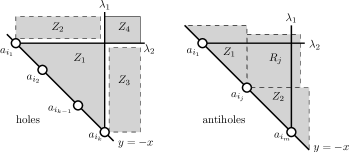
Figure 9: Proof of Theorem 5.4.

Now suppose the intersection graph $\mathcal{I}(\mathcal{R}_{\downarrow})$ has an odd-antihole $\mathcal{A}=\{R_{1},R_{2},\ldots,R_{k}\}$ of length at least 7. We keep the notation consistent from the odd-hole case; in particular, each $R_{i}$ does not intersect $R_{i-1}$ and $R_{i+1}$ (mod k). Assume that $a_{i_{1}}$ and $a_{i_{m}}$ are the leftmost and rightmost defining-corners in $A$, respectively. Using Figure 9 (right) as reference, it is easy to see that.

• Rectangles $R_{1}$ and $R_{m}$ are the only ones with corners $a_{1}$ and $a_{m}$, respectively: same argument as with odd-holes.

• Index $m\neq k$: if not, $R_{4}$ and $R_{5}$ would intersect both $R_{1}$ and $R_{m}$. Therefore, $\lambda_{1}\cap\lambda_{2}$ lies in $R_{4}\cap R_{5}$, which contradicts the intersecting structure of the antihole.

• Rectangles $R_{1}$ and $R_{m}$ intersect: this follows from $m\neq k$ (above) and $m\neq 2$ which is proved in the same way.

• There is a rectangle $R_{j}$ intersecting both $R_{1}$ and $R_{m}$ (because $k\geq 7$).

Rectangles $R_{j-1}$ and $R_{j+1}$ intersect each other, but do not intersect $R_{j}$, so they both lie either in zones $Z_{1}$ or in $Z_{2}$. This is a contradiction with the fact that $R_{j-1}$ and $R_{j+1}$ intersect $R_{1}$ and $R_{m}$. We conclude that $\mathcal{I}(\mathcal{R}_{\downarrow})$ has no odd-hole nor odd-antihole, and hence, it must be a perfect graph. ∎

In general, the intersection graph of inclusion-wise minimal rectangles in biconvex graphs is not always perfect (see Fig. 10). But the previous construction shows that the WMIS of biconvex graphs can be computed in polynomial time by solving a linear program.

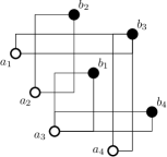
Figure 10: The intersection graph $\mathcal{I}(\mathcal{R}_{\downarrow})$ of a biconvex graph is not always perfect.

5.4 Convex BRFs

Recall that convex bipartite BRFs are the unrestricted BRFs with $A\subset L$ and $B\subseteq L^{+}$ with $L$ the diagonal line $y=-x$. Alternatively, they are the BRF graphs $G=(A\cup B,\mathcal{R})$ such that the points in $A$ are incomparable under $\leq_{\mathbb{R}^{2}}$. As we discuss in the next section, the maximum weight independent set of convex BRFs is equivalent to find the maximum weight point-interval set of a collection of intervals. For the latter problem, described in Section 6, Lubiw [41] provides a polynomial time algorithm that directly translates into an $O(n^{3})$-algorithm [52] for WMIS. Very recently, Correa et al. [21] improved Lubiw’s result, obtaining a $O(n^{2})$ algorithm.

Theorem 5.5.

[Based on [41, 21, 20]] We can compute a WMIS of a convex graph in $O(n^{3})$ using Lubiw’s algorithm for maximum weight point-interval set, and in quadratic time using the algorithm of Correa et al. [21].

5.5 Interval bigraphs

The natural geometric representation of an interval bigraph described at the beginning of the section is such that all the rectangles intersect the diagonal line $L$. We use this property and a recent result of Correa et al. [20] to strengthen Theorem 5.1 as follows.

Theorem 5.6.

Computing a WMIS of an interval bigraph is $\mathbf{NP}$-hard even for weights in $\{0,1\}$.

Proof.

The problem of computing a MIS of a family $\mathcal{I}$ of rectangles intersecting $L$ is $\mathbf{NP}$-hard [20]. Our hardness proof reduces from this problem, by transforming a collection of rectangles intersecting $L$ into a subset of rectangles of an interval bigraph (by translating and piecewise scaling the plane), and then using weights $\{0,1\}$ to distinguish the rectangles in the collection when solving the WMIS. The proof is very similar to that of Theorem 5.1. ∎

It is worth noting that currently, convex BRFs is the largest natural class of BRFs for which the WMIS problem is solvable in polynomial time. Nevertheless, Correa et al. [21, 20] gave a dynamic programming algorithm to compute WMIS of families of rectangles intersecting a diagonal line having the following property: if two rectangles intersect then they share a point below the diagonal. Based on this, they devise a 2-approximation for WMIS of rectangle families intersecting the diagonal whose running time is quadratic in the number of rectangles. Using their result we directly conclude that there exists an $O(n^{4})$ time algorithm to compute a 2-approximation for the WMIS of an interval bigraph.

6 Discussion

This section positions our results in the context of several closely related results for seemingly unrelated problems. In a nutshell, besides of greatly improving the algorithmic efficiency, our results greatly reduce the gap between the very complex algorithms, results and proofs for a generalization of our problem and the much simpler ones for a special case of our problem.

Let $G=(A\cup B,\mathcal{R})$ be a biconvex graph (see Section 5.1). Let $M^{G}$ be the biadjancency matrix whose rows and columns are sorted according to its corresponding biconvex labeling; note that the rows and columns of $M^{G}$ have their 1’s in consecutive position. We can identify the entries $M^{G}_{a,b}$ of value 1 with the rectangles $\Gamma(a,b)$ in the geometric representation of $G$. We can also identify a hitting point $p$ with the set of entries $M^{G}_{a,b}$ corresponding to rectangles hit by $p$; it turns out that all those sets must be block matrices with entries of value 1. The following two equivalences are easy to prove in the biconvex case: 1) a collection of entries of value 1 in $M^{G}$ induces an independent set of rectangles in $G$ if and only if no block matrix contains two of such entries; and 2) a set of points $p$ defines a hitting set in $G$ if and only if its corresponding set of block matrices cover all the 1’s in $M^{G}$. Chaiken et al. [11] show that the minimum size of a rectangle cover of a biconvex matrix $M$ (a set of block matrices covering all the 1’s in $M$) equals the maximum size of an antirectangle (a set of 1’s in $M$ such that no block matrix contains two of them); this corresponds to Theorem 4.3 for biconvex graphs.

Going up to convex graphs, the work of Györi [34] on point-interval pairs is particularly relevant. He works with a fixed ground set $A=\{1,\ldots,n\}$, intervals $I\subseteq A$ and point-interval pairs $(p,I)$ where $p\in I\subseteq A$. He introduces two notions: 1) a family of intervals $\mathcal{B}$ is a basis for another family of intervals $\mathcal{F}$, if every interval of $\mathcal{F}$ can be written as union of intervals in $\mathcal{B}$; and 2) a collection of point-interval pairs $(p_{i},I_{i})_{i=1..m}$ is called independent if, for all $j\neq k$, either $p_{j}\notin I_{k}$ or $p_{k}\notin I_{j}$. Györi proves, non-constructively, that the cardinality of minimum basis for a family $\mathcal{F}$ equals the maximum cardinality of an independent family of point-interval pairs $(p,I)$, where $I$ is restricted to be in $\mathcal{F}$. To put this min-max result in our context, note that the containment relation on $(A\times\mathcal{F})$ defines a convex graph on $A$. Through the representation of convex BRFs used in Section 5.4, we can represent $A$ as a set of points in the antidiagonal line $y=-x$, while we can represent $\mathcal{F}$ as points weakly above this line. The rectangles in the convex graph $(A\cup\mathcal{F},\mathcal{R})$ become the set of all point-interval pairs $(p,I)$ where $I\in F$. It is easy to see that independent set of rectangles are in correspondence with independent families of point-interval pairs. Hitting sets of rectangles are also in correspondence with minimum basis of intervals, although not bijectively: we identify $q$ with the interval $I_{q}$ of points $a\in A$ with $a\leq_{\mathbb{R}^{2}}q$; a hitting set $H$ is transformed into a basis $\{I_{q}:q\in H\}$ for $\mathcal{F}$ since $I=\cup_{q\in H,q\leq_{\mathbb{R}^{2}}I}I_{q}$ for all $I\in F$. On the other hand, a basis for $\mathcal{F}$ induces a hitting set $H$ for $\mathcal{R}$ of the same cardinality, through the inverse identification.

The equivalences just described show that Györi’s min-max result on point-interval pairs implies Theorem 4.3 for convex graphs, and also that Lubiw’s algorithm [41] for weighted independent set of point-interval pairs implicitly provides an algorithm for the maximum weighted independent set of rectangles in convex BRFs, as described in Theorem 5.5. Furthermore, Györi [34] also shows that for convex matrices (i.e., where the 1’s on each column are consecutive), the minimum size of a rectangle cover equals the maximum size of an antirectangle, thus extending the min-max result of Chaiken [11]. This indeed follows from Theorem 4.3 for convex graphs, through a simple geometric argument we skip here [34].

Following Györi’s non-constructive proof, there was significant interest in obtaining a constructive, simple and efficient version of his min-max result, and their generalizations. Franzblau and Kleitman [31] present an algorithmic proof that uses the original ideas from Györi. Later, Frank [29] presents an alternative algorithmic proof using new ideas, which form the core of Algorithm 1: interpreting his algorithm in our geometric setting, the procedure starts from a convex BRF $G=(A\cup B,\mathcal{R})$, determines a cross-free intersection family $\mathcal{K}\subseteq\mathcal{R}$, and then uses Dilworth’s theorem to determine a maximum independent set and a hitting set of $\mathcal{K}$, which then manages to transform into a maximum independent set and a hitting set of $\mathcal{R}$. After the additional improvements in [6], the theoretical performance of the algorithm of Franzblau and Kleitman is better than the one of Frank, providing running times of $O(n^{2})$ and $O(n^{2.5}\log^{3/2}n)$ for the minimum hitting set and the maximum independent set of convex BRFs, respectively.

A concrete contribution of our work is to adapt the Frank’s algorithm to the much broader set of BRFs, with no additional overhead in the running time. We remark that although we use some ideas from [6] to tweak the algorithm, our case is significantly more complex.

The algorithm of Frank was not developed only in pursuit of a clean algorithmic version of the theorem of Gyori (which anyway was already given by Franzblau and Kleitman). A few years earlier, Frank and Jordán [30] had presented a much more general min-max theorem which encompassed all the special cases above, including the case of BRFs. The description of this theorem, in principle, is much more abstract. A collection of pairs of sets $(S_{i},T_{i})$ is half-disjoint if for every $j\neq k$, either $S_{j}\cap S_{k}$ or $T_{j}\cap T_{k}$ are empty. A directed-edge $(s,t)$ covers a set-pair $(S,T)$ if $s\in S$ and $t\in T$. A family $\mathcal{S}$ of set-pairs is crossing if whenever $(S,T)$ and $(S^{\prime},T^{\prime})$ are in $\mathcal{S}$, so are $(S\cap T,S^{\prime}\cup T^{\prime})$ and $(S\cup T,S^{\prime}\cap T^{\prime})$. Frank and Jordán show that for every crossing family $\mathcal{S}$, the maximum size of a half-disjoint subfamily is equal to the minimum size of a collection of directed-edges covering $\mathcal{S}$. Even further, the proof they offer was algorithmic, even though it relied on the ellipsoid method.

Our min-max result follows from Frank and Jordán’s theorem: the inclusionwise minimal rectangles $\mathcal{R}_{\downarrow}$ of a BRF $(A\cup B,\mathcal{R})$, once projected over both axes $\{(R_{x},R_{y}):R\in\mathcal{R}_{\downarrow}\}$, becomes a crossing family of set-pairs for which half-disjoint subfamilies become independent sets in $\mathcal{R}$, while coverings by directed edges become hitting sets in $\mathcal{R}$. Thus, it may seem that our contribution is merely that of an algorithmic improvement. Yet, the literature that followed [30] shows why this is not the case. The generality of Frank and Jordán also carries significantly more abstract concepts, algorithms and proofs. Already the work of Frank  [29] and Benczúr et al. [6] show that a significant effort is required in order to translate the original ideas of Frank and Jordán [30] into an efficient and intuitive algorithmic proof for the theorem of Györi. More recently, the combinatorial algorithm of Benczur [7] for pairs of sets gives a more intuitive view of these objects, but still both the algorithm and the analysis are still much more complex and abstract than ours. The algorithmic proof we provide for Theorem 4.3 has the value of positioning BRFs at the same level of complexity than the convex BRFs studied by Györi, both conceptually and algorithmically, for the problems we are concerned here.

It is worth noting that the min-max result also apply to BRFs that are drawn in a cylinder $\mathbb{S}^{1}\times\mathbb{R}$ or a torus $\mathbb{S}^{1}\times\mathbb{S}^{1}$. In both surfaces axis-aligned rectangles are well-defined as cartesian products of closed intervals. Given two finite sets of points $A$ and $B$ and an arbitrary set $\mathcal{Z}$ in a surface $\mathcal{S}$ that can be either a cylinder or a torus, we can still define the collection $\mathcal{R}_{\downarrow}$ of inclusionwise minimal axis-aligned rectangles contained in $\mathcal{Z}$ with lower left corner in $A$ and upper right corner in $B$. It is easy to see that $\{(R_{x},R_{y})\colon R_{x}\times R_{y}\in\mathcal{R}_{\downarrow}\}$ is a crossing family of set-pairs. Applying Frank and Jordán theorem, the size of a maximum independent set in $\mathcal{R}_{\downarrow}$ equals the size of a minimum hitting set. We believe it is not hard to modify our combinatorial algorithm to work in this case too, but we defer this to future work.

7 Acknowledgements

The first author was partially supported by Nucleo Milenio Información y Coordinación en redes ICM/FIC P10-024F and by CONICYT via FONDECYT grant 11130266. The second author was partially supported by the FSR Incoming Post-doctoral Fellowship of the Catholic University of Louvain (UCL), funded by the French Community of Belgium. The authors gratefully acknowledge Prof. Andreas S. Schulz for many stimulating discussions during the early stages of this paper.

References

- [1] A. Adamaszek, A. Wiese, Approximation schemes for maximum weight independent set of rectangles, in: FOCS 2013.
- [2] P. Agarwal, M. Van Kreveld, S. Suri, Label placement by maximum independent set in rectangles, Computational Geometry 11 (3) (1998) 209–218.
- [3] P. K. Agarwal, N. H. Mustafa, Independent set of intersection graphs of convex objects in 2D, Comput. Geom. 34 (2) (2006) 83–95.
- [4] J. Amilhastre, P. Janssen, M.-C. Vilarem, Computing a minimum biclique cover is polynomial for bipartite domino-free graphs, in: SODA, 1997.
- [5] B. Aronov, E. Ezra, M. Sharir, Small-size -nets for axis-parallel rectangles and boxes, SIAM J. Comput. 39 (7) (2010) 3248–3282.
- [6] A. Benczúr, J. Förster, Z. Király, Dilworth’s theorem and its application for path systems of a cycle. implementation and analysis, in: J. Nešetřil (ed.), Algorithms - ESA’ 99, vol. 1643 of Lecture Notes in Computer Science, Springer Berlin / Heidelberg, 1999, pp. 693–693.
- [7] A. A. Benczúr, Pushdown-reduce: an algorithm for connectivity augmentation and poset covering problems, Discrete Applied Mathematics 129 (2-3) (2003) 233–262.
- [8] A. Brandstädt, The jump number problem for biconvex graphs and rectangle covers of rectangular regions, in: J. Csirik, J. Demetrovics, F. Gécseg (eds.), Fundamentals of Computation Theory, vol. 380 of Lecture Notes in Computer Science, Springer, 1989.
- [9] A. Brandstädt, V. B. Le, J. P. Spinrad, Graph classes: a survey, Society for Industrial and Applied Mathematics, Philadelphia, PA, USA, 1999.
- [10] H. Brönnimann, M. Goodrich, Almost optimal set covers in finite VC-dimension, Discrete & Computational Geometry 14 (1995) 463–479, 10.1007/BF02570718.
- [11] S. Chaiken, D. J. Kleitman, M. Saks, J. Shearer, Covering regions by rectangles, SIAM Journal on Algebraic and Discrete Methods 2 (4) (1981) 394–410.
- [12] P. Chalermsook, Coloring and maximum independent set of rectangles, in: L. A. Goldberg, K. Jansen, R. Ravi, J. D. P. Rolim (eds.), APPROX-RANDOM, vol. 6845 of Lecture Notes in Computer Science, Springer, 2011.
- [13] P. Chalermsook, J. Chuzhoy, Maximum independent set of rectangles, in: C. Mathieu (ed.), SODA, SIAM, 2009.
- [14] T. Chan, Polynomial-time approximation schemes for packing and piercing fat objects, Journal of Algorithms 46 (2) (2003) 178–189.
- [15] T. M. Chan, S. Har-Peled, Approximation algorithms for maximum independent set of pseudo-disks, Discrete & Computational Geometry 48 (2) (2012) 373–392.
- [16] T. M. Chan, A.-A. Mahmood, Approximating the piercing number for unit-height rectangles, in: CCCG, 2005.
- [17] G. Chaty, M. Chein, Ordered matchings and matchings without alternating cycles in bipartite graphs, Utilitas Math 16 (1979) 183–187.
- [18] M. Chudnovsky, N. Robertson, P. Seymour, R. Thomas, The strong perfect graph theorem, Annals of Mathematics (2006) 51–229.
- [19] B. Cohen, S. Skiena, Optimizing combinatorial library construction via split synthesis, in: RECOMB, 1999.
- [20] J. R. Correa, L. Feuilloley, P. Perez-Lantero, J. A. Soto, Independent and hitting sets of rectangles intersecting a diagonal line : Algorithms and complexity, Unpublished manuscript. Submitted.
- [21] J. R. Correa, L. Feuilloley, J. A. Soto, Independent and hitting sets of rectangles intersecting a diagonal line, in: A. Pardo, A. Viola (eds.), LATIN 2014: Theoretical Informatics - 11th Latin American Symposium, Montevideo, Uruguay, March 31 - April 4, 2014. Proceedings, Springer, 2014.
- [22] E. Dahlhaus, The computation of the jump number of convex graphs, in: V. Bouchitté, M. Morvan (eds.), ORDAL, vol. 831 of Lecture Notes in Computer Science, Springer, 1994.
- [23] J. Doerschler, H. Freeman, A rule-based system for dense-map name placement, Communications of the ACM 35 (1) (1992) 68–79.
- [24] T. Erlebach, K. Jansen, E. Seidel, Polynomial-time approximation schemes for geometric graphs, in: Proceedings of the twelfth annual ACM-SIAM symposium on Discrete algorithms, Society for Industrial and Applied Mathematics, 2001.
- [25] H. Fauck, Covering polygons with rectangles via edge coverings of bipartite permutation graphs, Elektronische Informationsverarbeitung und Kybernetik 27 (8) (1991) 391–409.
- [26] L. Ford, D. Fulkerson, Flow in networks, Princeton University Press Princeton, 1962.
- [27] R. Fowler, M. Paterson, S. Tanimoto, Optimal packing and covering in the plane are np-complete, Information processing letters 12 (3) (1981) 133–137.
- [28] A. Frank, Finding minimum generators of path systems, J. Comb. Theory, Ser. B 75 (2) (1999) 237–244.
- [29] A. Frank, Finding minimum weighted generators of a path system, in: J. N. Ronald L. Graham, Jan Kratochvíl, F. S. Roberts (eds.), Contemporary Trends in Discrete Mathematics, vol. 49 of DIMACS Series in Discrete Mathematics and Theoretical Computer Science, American Mathematical Society, 1999, pp. 129–137.
- [30] A. Frank, T. Jordán, Minimal edge-coverings of pairs of sets, J. Comb. Theory, Ser. B 65 (1) (1995) 73–110.
- [31] D. S. Franzblau, D. J. Kleitman, An algorithm for constructing regions with rectangles: Independence and minimum generating sets for collections of intervals, in: STOC, 1984.
- [32] D. S. Franzblau, D. J. Kleitman, An algorithm for covering polygons with rectangles, Information and Control 63 (3) (1984) 164–189.
- [33] T. Fukuda, Y. Morimoto, S. Morishita, T. Tokuyama, Data mining with optimized two-dimensional association rules, ACM Trans. Database Syst. 26 (2) (2001) 179–213.
- [34] E. Györi, A minimax theorem on intervals, J. Comb. Theory, Ser. B 37 (1) (1984) 1–9.
- [35] J. Hopcroft, R. Karp, An n^5/2 algorithm for maximum matchings in bipartite graphs, SIAM Journal on Computing 2 (4) (1973) 225–231.
- [36] H. Imai, T. Asano, Finding the connected components and a maximum clique of an intersection graph of rectangles in the plane, Journal of algorithms 4 (4) (1983) 310–323.
- [37] E. Kushilevitz, N. Nisan, Communication complexity, Cambridge University Press, New York, NY, USA, 1997.
- [38] B. Lent, A. Swami, J. Widom, Clustering association rules, in: Data Engineering, 1997. Proceedings. 13th International Conference on, IEEE, 1997.
- [39] L. Lewin-Eytan, J. Naor, A. Orda, Routing and admission control in networks with advance reservations, Approximation Algorithms for Combinatorial Optimization (2002) 215–228.
- [40] L. Lovász, A characterization of perfect graphs, Journal of Combinatorial Theory, Series B 13 (2) (1972) 95–98.
- [41] A. Lubiw, A weighted min-max relation for intervals, J. Comb. Theory, Ser. B 53 (2) (1991) 151–172.
- [42] M. Mucha, P. Sankowski, Maximum matchings via gaussian elimination, in: Foundations of Computer Science, 2004. Proceedings. 45th Annual IEEE Symposium on, IEEE, 2004.
- [43] H. Müller, Alternating cycle-free matchings, Order 7 (1990) 11–21.
- [44] H. Müller, On edge perfectness and classes of bipartite graphs, Discrete Mathematics 149 (1-3) (1996) 159–187.
- [45] H. Müller, Recognizing interval digraphs and interval bigraphs in polynomial time, Discrete Applied Mathematics 78 (1) (1997) 189–205.
- [46] N. H. Mustafa, S. Ray, Improved results on geometric hitting set problems, Discrete & Computational Geometry 44 (4) (2010) 883–895.
- [47] D. S. Nau, G. Markowsky, M. A. Woodbury, D. B. Amos, A mathematical analysis of human leukocyte antigen serology, Mathematical Biosciences 40 (3-4) (1978) 243–270.
- [48] J. Orlin, Contentment in graph theory: Covering graphs with cliques, Indagationes Mathematicae (Proceedings) 80 (5) (1977) 406–424.
- [49] W. R. Pulleyblank, Alternating cycle free matchings, Tech. Rep. CORR 82-18, University of Waterloo - Dept. of Combinatorics and Optimization (1982).
- [50] A. Schrijver, Combinatorial optimization: polyhedra and efficiency, vol. 24, Springer, 2003.
- [51] A. M. Shrestha, S. Tayu, S. Ueno, On two-directional orthogonal ray graphs, in: Proceedings of 2010 IEEE International Symposium on Circuits and Systems (ISCAS), 2010.
- [52] J. Soto, C. Telha, Jump number of two-directional orthogonal ray graphs, Integer Programming and Combinatoral Optimization (2011) 389–403.
- [53] J. P. Spinrad, Efficient Graph Representations.: The Fields Institute for Research in Mathematical Sciences., vol. 19, American Mathematical Soc., 2003.
- [54] G. Steiner, L. K. Stewart, A linear time algorithm to find the jump number of 2-dimensional bipartite partial orders, Order 3 (1987) 359–367.
- [55] D. E. Willard, G. S. Lueker, Adding range restriction capability to dynamic data structures, J. ACM 32 (3) (1985) 597–617.
- [56] V. V. Williams, Multiplying matrices faster than Coppersmith-Winograd, in: STOC, 2012.