A power-law decay model with autocorrelation for posting data to social networking services

Abstract

We propose a power-law decay model with autocorrelation for posting data to social networking services concerning particular events such as national holidays or major sport events. In these kinds of events we observe people’s interest both before and after the events. In our model the number of postings has a Poisson distribution whose expected value decays as a power law. Our model also incorporates autocorrelations by autoregressive specification of the expected value. We show that our proposed model well fits the data from social networking services.

Keywords and phrases:  conditional Poisson autoregressive model, Fisher information, number of postings.

1 Introduction

With the increasing usage of social networking services (SNS), such as many blog services, Facebook or Twitter, it is important to obtain information from postings to these services. We look at the data on the number of postings for various events, such as national holidays or major sport events. By analyzing the data, we gain insights on how a particular topic interests people, how actively it is discussed around the date of the event and how long the memory of the event lasts. Our data is time series data, but the length of the series is usually short, covering several weeks before and after the event. It is far from stationary, because there is a sharp peak of the number of postings on the date of the event.

Many studies on posting data to SNS focus on the network structure of the services (e.g. [2], [9], [12]), such as how certain topic spreads by interaction among users of the services. In this paper we study the pattern of number of postings concerning particular events, such as national holidays or major sport events. The events we study are scheduled events, so that people are aware when the events will happen. This contrasts with unpredictable events, such as the occurrence of large earthquakes ([11]). In the case of unpredictable events, we only observe effects of the event after it happens. On the other hand, in the case of the scheduled events, the number of postings depends on people’s anticipation of the event and the after-effect of the actual outcome of the event. Another similar type of data studied in literature is the registration data until the deadline for events such as academic conferences (e.g. [1], [4]). In this kind of data, we only observe people’s actions before the deadline.

We combine the model of the mean number of postings proposed in [10] and the conditional Poisson autoregressive (AR) models for count data. The conditional Poisson autoregressive models are applied in many problems in econometrics, political science or epidemiology (e.g. [8], [3]). For a theoretical survey of the conditional Poisson autoregressive model see [6], [5] and [7]. Zhu ([13]) generalized the conditional Poisson model to generalized Poisson integer-valued GARCH models. By our model we can better predict how people’s interest on particular events decays with time and our model is useful for example in designing advertisement strategy for web marketing.

In the left graph of Figure 1 we show a typical symmetric pattern of number of postings. Tokyo Marathon 2014 was held on Sunday, February 23 of 2014. It was well anticipated and it ended without unexpected happenings. In these cases, the number of postings shows a symmetric pattern with a sharp peak on the date of the event. Both sides of the peak seems to exhibit a behavior of some negative power in the time difference from the actual date of the event. Also there is some stochastic fluctuation of the number of postings. This is the motivation of our proposed model.

Tokyo Marathon 2014                        Silver medal by Kasai

Figure 1: Symmetric and asymmetric patterns

A different asymmetric pattern is observed, when there is some surprising element of the event. In the right graph of Figure 1 we show the data on Noriaki Kasai around February 16, 2014, when he won a silver medal in ski jump in 2014 winter Olympics. From the data we see that people did not anticipate the medal before the event.

The organization of this paper is as follows. In Section 2 we propose to model the mean of the number of postings by a power-law decay model with three parameters and we assume independent Poisson distributions. We also study the Fisher information matrix under the proposed model. In Section 3 we incorporate autocorrelation to our model by conditional Poisson autoregression. In Section 4 we apply our model to some social networking service data in Japan. We end the paper with some discussion in Section 5.

2 A power-law decay model for the mean number of postings

Let $t_{0}$ denote the date of the event and let $y_{t}$ denote the number of postings on the event on day $t$. We model the expected value of $y_{t}$ by the following power-law decay function.

$$E(y_{t})=\mu_{t}(\alpha,\beta,\gamma)=\gamma\frac{1}{(\alpha|t-t_{0}|+1)^{\beta}}.$$ (1)

This power-law decay model was proposed by [10] without the parameter $\alpha$. They used the least-squares method, while we use the maximum likelihood estimation. They do not consider fitting the data close to the peak, which becomes possible by introducing the parameter $\alpha$.

The interpretation of the parameters is as follows.

$\alpha$: steepness of the curve just before and after the event

$\beta$: longer decay pattern

$\gamma$: impact of the event (peak level, the maximum number of postings)

In this section we assume that $y_{t}$, $t=t_{L},t_{L}+1,\dots,t_{U}-1,t_{U}$, $t_{L}\leq t_{0}\leq t_{U}$, are independent Poisson random variables with the mean given by $\mu_{t}(\alpha,\beta,\gamma)$ in (1). We call the model “power-law decay independence model”. We denote the probability function of the Poisson distribution with the mean $\mu$ as

$${\rm Po}(y\mid\mu)=\frac{\mu^{y}}{y!}e^{-\mu}.$$ (2)

Then the likelihood function is written as

$$L(\alpha,\beta,\gamma)=\prod_{t=t_{L}}^{t_{U}}{\rm Po}(y_{t}\mid\mu_{t}(\alpha,\beta,\gamma))=\prod_{t=t_{L}}^{t_{U}}\frac{\mu_{t}(\alpha,\beta,\gamma)^{y_{t}}}{{y_{t}}!}e^{-\mu_{t}(\alpha,\beta,\gamma)}.$$ (3)

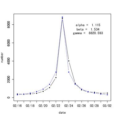
Figure 2: Fitting the power-law decay independence model to Tokyo Marathon data

We found that the maximization of the log-likelihood function is numerically very simple. We give a typical example of maximum likelihood estimation (MLE) of (3) in Figure 2. In Figure 2 the solid line is the observed data and the the dotted line is the fitted curve of expected values by MLE. We use the same distinction of line types in Figures 3 and 4. The estimates are $\hat{\alpha}=1.115$, $\hat{\beta}=1.534$ and $\hat{\gamma}=8820.593$. Our model seems to fit the data well, but there is a slight asymmetry in this data, which is not captured by the symmetric model in (1).

We will discuss many examples of fitting of (3) and its generalizations later in Section 4.

2.1 Fisher information matrix for the independence model

As we already noted in the beginning, the length of our data is not very large and our data is far from stationary. Hence the usual asymptotics for the length of the series is not appropriate. Nevertheless it is of theoretical interest to consider the behavior of MLE of (3) as the length of the series diverges to infinity. On the other hand we have large number of postings $y_{t_{0}}$ on the date $t_{0}$ of the event. Under our model of Poisson distribution, we can also think of the asymptotics, where $\gamma=E(y_{t_{0}})$ diverges to infinity. In the following we calculate the Fisher information matrix

$$I=\begin{pmatrix}I_{\alpha\alpha}&I_{\alpha\beta}&I_{\alpha\gamma}\\ I_{\alpha\beta}&I_{\beta\beta}&I_{\beta\gamma}\\ I_{\alpha\gamma}&I_{\beta\gamma}&I_{\gamma\gamma}\end{pmatrix},$$

for our model to gain insights on the behavior of MLE for the model (3).

For notational simplicity let $t_{0}=0$ and $t_{L}\leq 0\leq t_{U}$. Then the log-likelihood function $l(\alpha,\beta,\gamma)=\log L(\alpha,\beta,\gamma)$ is written as

$$l(\alpha,\beta,\gamma) =\sum_{t=t_{L}}^{t_{U}}(y_{t}\log\mu_{t}(\alpha,\beta,\gamma)-\mu_{t}(\alpha,\beta,\gamma)-\log y_{t}!)$$

$$=\sum_{t=t_{L}}^{t_{U}}\Big{(}y_{t}(\log\gamma-\beta\log(\alpha|t|+1))-\gamma\frac{1}{(\alpha|t|+1)^{\beta}}-\log y_{t}!\Big{)}$$

$$=C+\log\gamma\sum_{t=t_{L}}^{t_{U}}y_{t}-\beta\sum_{t=t_{L}}^{t_{U}}y_{t}\log(\alpha|t|+1)-\gamma\sum_{t=t_{L}}^{t_{U}}\frac{1}{(\alpha|t|+1)^{\beta}},$$

where $C$ does not depend on parameters. Then

$$-\frac{\partial^{2}}{\partial\alpha^{2}}l=-\beta\sum_{t=t_{L}}^{t_{U}}y_{t}\frac{|t|^{2}}{(\alpha|t|+1)^{2}}+\gamma\beta(\beta+1)\sum_{t=t_{L}}^{t_{U}}\frac{|t|^{2}}{(\alpha|t|+1)^{\beta+2}}.$$

The expected value of this second derivative is given as

$$I_{\alpha\alpha}=E[-\frac{\partial^{2}}{\partial\alpha^{2}}l] =-\beta\gamma\sum_{t=t_{L}}^{t_{U}}\frac{|t|^{2}}{(\alpha|t|+1)^{\beta+2}}+\gamma\beta(\beta+1)\sum_{t=t_{L}}^{t_{U}}\frac{|t|^{2}}{(\alpha|t|+1)^{\beta+2}}$$

$$=\gamma\beta^{2}\sum_{t=t_{L}}^{t_{U}}\frac{|t|^{2}}{(\alpha|t|+1)^{\beta+2}}.$$

Note that $I_{\alpha\alpha}\rightarrow\infty$ as $\gamma=E(y_{0})\rightarrow\infty$. However, when $\gamma$ is fixed

$$\lim_{\max(-t_{L},t_{U})\rightarrow\infty}I_{\alpha\alpha}=\infty\ \ \Leftrightarrow\ \ \beta\leq 1\ \ \Leftrightarrow\ \ \sum_{t=t_{L}}^{t_{U}}E\left(y_{t}\right)\rightarrow\infty.$$

Next consider $I_{\alpha\beta}$. Noting

$$(\alpha t+1)^{-\beta}=\exp(-\beta\log(\alpha t+1))$$

and

$$\frac{\partial}{\partial\beta}(\alpha t+1)^{-\beta}=-\log(\alpha t+1)\exp(-\beta\log(\alpha t+1))=-\log(\alpha t+1)\frac{1}{(\alpha t+1)^{\beta}},$$

we have

$$-\frac{\partial^{2}}{\partial\alpha\partial\beta}l =\frac{\partial}{\partial\alpha}\left[\sum_{t=t_{L}}^{t_{U}}y_{t}\log(\alpha|t|+1)-\gamma\sum_{t=t_{L}}^{t_{U}}\log(\alpha|t|+1)\frac{1}{(\alpha|t|+1)^{\beta}}\right]$$

$$=\sum_{t=t_{L}}^{t_{U}}y_{t}\frac{|t|}{\alpha|t|+1}-\gamma\sum_{t=t_{L}}^{t_{U}}\frac{|t|}{(\alpha|t|+1)^{\beta+1}}+\gamma\beta\sum_{t=t_{L}}^{t_{U}}\log(\alpha|t|+1)\frac{|t|}{(\alpha|t|+1)^{\beta+1}}.$$

When we take the expected value, the first two terms cancel and

$$I_{\alpha\beta}=E[-\frac{\partial^{2}}{\partial\alpha\partial\beta}l]=\beta\gamma\sum_{t=t_{L}}^{t_{U}}\log(\alpha|t|+1)\frac{|t|}{(\alpha|t|+1)^{\beta+1}}.$$

The divergence is the same as in the case of $I_{\alpha\alpha}$.

Similarly we can evaluate $I_{\beta\beta},I_{\alpha\gamma},I_{\beta\gamma},I_{\gamma\gamma}$ as

$$I_{\beta\beta} =\gamma\sum_{t=t_{L}}^{t_{U}}\frac{(\log(\alpha|t|+1))^{2}}{(\alpha|t|+1)^{\beta}},\qquad I_{\alpha\gamma}=-\beta\sum_{t=t_{L}}^{t_{U}}\frac{|t|}{(\alpha|t|+1)^{\beta+1}},$$

$$I_{\beta\gamma} =-\sum_{t=t_{L}}^{t_{U}}\frac{\log(\alpha|t|+1)}{(\alpha|t|+1)^{\beta}},\qquad I_{\gamma\gamma}=\frac{1}{\gamma}\sum_{t=t_{L}}^{t_{U}}\frac{1}{(\alpha|t|+1)^{\beta}}.$$

Although it is tedious to prove the consistency and the asymptotic normality of MLE based only on the computation of Fisher information matrix, our computation suggests the following results. Since $y_{t_{0}}$ has the Poisson distribution with the mean $\gamma$ and the standard deviation $\sqrt{\gamma}$, $y_{t_{0}}/\gamma$ converges to 1 in probability as $\gamma\rightarrow\infty$. In fact, when we compute MLE, $\gamma$ is basically estimated by $y_{t_{0}}$, since the number of postings has a sharp peak at $t=t_{0}$ (see Figure 2). Furthermore $I_{\alpha\alpha},I_{\alpha\beta},I_{\beta\beta}$ are linear in $\gamma$. This suggests that MLE is consistent as $\gamma\rightarrow\infty$. For large expected value, Poisson distribution is approximately by normal distribution after normalization. Hence the score functions $\partial l/\partial\alpha,\partial l/\partial\beta,\partial l/\partial\gamma$ are approximately normally distributed as $\gamma\rightarrow\infty$. The confidence intervals given in Section 4 are based on this approximation. When $\gamma$ is fixed and $\max(-t_{L},t_{U})\rightarrow\infty$, the elements of the Fisher information matrix diverge to $\infty$ if and only if $\beta\leq 1$, or equivalently $\sum_{t=t_{L}}^{t_{U}}E(y_{t})\rightarrow\infty$.

3 Conditional Poisson regression modeling for autocorrelations

In the last section we assumed that the number of postings $y_{t}$ are independent. We generalize this model to allow autocorrelations by conditional Poisson regression modeling. As we saw, the estimate of the parameter $\gamma$ in (1) is very close to $y_{t_{0}}$. Hence in this section we replace $\gamma$ by $y_{t_{0}}$. This is the initial value of our autoregressive scheme and we model the number of postings after the event $y_{t}$, $t>t_{0}$.

Concerning the data $y_{t}$, $t<t_{0}$, before the date of the event, we can use the model given in (4) by reversing the time axis. This is similar to look at the standard AR(1) process

$$x_{t}=\rho x_{t-1}+\epsilon_{t}$$

in the reverse time direction by taking the reciprocal of the autoregressive coefficient $\rho$. However this modeling of the data before the date of the event is somewhat unsatisfactory, in particular for the purpose of predicting $y_{t_{0}}$ before the date of the event. We discuss this point again in Section 5.

We replace $\gamma$ by $y_{t_{0}}$ in (1) and regard it as the conditional expected value of $y_{t}$ given $y_{t_{0}}$

$$E(y_{t}|y_{t_{0}})=y_{t_{0}}\frac{1}{(\alpha|t-t_{0}|+1)^{\beta}},\quad t\geq t_{0}.$$

Then $E(y_{t}|y_{t_{0}})$ is recursively written as

$$E(y_{t}|y_{t_{0}}) =E(y_{t-1}|y_{t_{0}})\left(\frac{(|t-t_{0}|-1)\alpha+1}{|t-t_{0}|\alpha+1}\right)^{\beta}$$

$$=E(y_{t-2}|y_{t_{0}})\left(\frac{(|t-t_{0}|-2)\alpha+1}{|t-t_{0}|\alpha+1}\right)^{\beta}$$

$$=\dots$$

We propose the following AR(2) type modeling of $y_{t},t\geq t_{0}+2$:

$$p(y_{t_{0}+1}|y_{t_{0}}) ={\rm Po}\left(y_{t_{0}+1}\mid y_{t_{0}}\frac{1}{(\alpha+1)^{\beta}}\right)$$

$$p(y_{t_{0}+2}|y_{t_{0}+1},y_{t_{0}}) ={\rm Po}\left(y_{t_{0}+2}\mid s\times y_{t_{0}+1}\left(\frac{\alpha+1}{2\alpha+1}\right)^{\beta}+(1-s)\times y_{t_{0}}\left(\frac{1}{2\alpha+1}\right)^{\beta}\right)$$

$$p(y_{t_{0}+3}|y_{t_{0}+2},y_{t_{0}+1}) ={\rm Po}\left(y_{t_{0}+3}\mid s\times y_{t_{0}+2}\left(\frac{2\alpha+1}{3\alpha+1}\right)^{\beta}+(1-s)\times y_{t_{0}+1}\left(\frac{\alpha+1}{3\alpha+1}\right)^{\beta}\right)$$

$$\ \vdots$$

$$p(y_{t_{0}+m}|y_{t_{0}+m-1},y_{t_{0}+m-2}) ={\rm Po}\left(y_{t_{0}+m}\mid s\times y_{t_{0}+m-1}\left(\frac{(m-1)\alpha+1}{m\alpha+1}\right)^{\beta}\right.$$

$$\qquad+\left.(1-s)\times y_{t_{0}+m-2}\left(\frac{(m-2)\alpha+1}{m\alpha+1}\right)^{\beta}\right).$$ (4)

Note that $y_{t_{0}+1}$ is given in an AR(1) form. Then the conditional likelihood function for $\alpha,\beta,s$ given $y_{t_{0}}$ for the data $y_{t_{0}+1},\dots,y_{t_{0}+T}$ is written as

$$L(\alpha,\beta,s) ={\rm Po}\left(y_{t_{0}+1}\mid y_{t_{0}}\frac{1}{(\alpha+1)^{\beta}}\right)$$

$$\quad\times\prod_{m=2}^{T}{\rm Po}\left(y_{t_{0}+m}\mid s\times y_{t_{0}+m-1}\left(\frac{(m-1)\alpha+1}{m\alpha+1}\right)^{\beta}+(1-s)\times y_{t_{0}+m-2}\left(\frac{(m-2)\alpha+1}{m\alpha+1}\right)^{\beta}\right).$$ (5)

When $s=1$, we have an AR(1) form. When we estimate $s$ in $L(\alpha,\beta,s)$, we restrict $s\in[0,1]$, although for some data sets unrestricted MLE of $s$ happened to be larger than 1.

Note that the independence model in (3) and the AR(2) model in (5) are separate models. In the usual AR(1) model of continuous observations $x_{t}=\rho x_{t-1}+\epsilon_{t}$, the independence model is a special case of $\rho=0$. In order to interpolate between the independence model (3) and the AR(2) model (5), we propose the following more generalized and unifying model with the new parameters $u,v\in[0,1]$ representing the weights of the two models.

$$p(y_{t_{0}+m}|y_{t_{0}+m-1},y_{t_{0}+m-2})$$

$$\qquad={\rm Po}\Biggl{(}y_{t_{0}+m}\mid w\times\left(\frac{y_{t_{0}}}{((m-1)\alpha+1)^{\beta}}\right)^{u}\left(y_{t_{0}+m-1}\right)^{1-u}\times\left(\frac{(m-1)\alpha+1}{m\alpha+1}\right)^{\beta}$$

$$\qquad\ \ +(1-w)\times\left(\frac{y_{t_{0}}}{((m-2)\alpha+1)^{\beta}}\right)^{v}\left(y_{t_{0}+m-2}\right)^{1-v}\times\left(\frac{(m-2)\alpha+1}{m\alpha+1}\right)^{\beta}\Biggl{)}.$$ (6)

In this unifying model, $u$ is the weight for the lag one term and $v$ is the weight for the lag two term. We introduced these two parameters separately for flexibility of the model.

3.1 Fisher information matrix for the AR(1) model

Here we evaluate Fisher information matrix for AR(1) model, i.e. the model in (5) with $s=1$. We let $t_{0}=0$ for simplicity and assume that $y_{0},\dots,y_{T}$ are observed. We also replace $\gamma$ by $y_{0}$ and consider the conditional likelihood in $\alpha$ and $\beta$ given $y_{0}$.

The conditional expected values given $y_{0}$ are evaluated as

$$\begin{split}E[y_{1}|y_{0}]&=y_{0}\left(\frac{1}{\alpha+1}\right)^{\beta},\\ E[y_{2}|y_{1}]&=y_{1}\left(\frac{\alpha+1}{2\alpha+1}\right)^{\beta},\ \ E^{y_{1}}[E[y_{2}|y_{1}]|y_{0}]=E[y_{2}|y_{0}]=y_{0}\left(\frac{1}{2\alpha+1}\right)^{\beta},\\ &\vdots\\ E[y_{t}|y_{t-1}]&=y_{t-1}\left(\frac{(t-1)\alpha+1}{t\alpha+1}\right)^{\beta},\ \ E^{y_{t-1}}[E[y_{t}|y_{t-1}]|y_{0}]=E[y_{t}|y_{0}]=y_{0}\left(\frac{1}{t\alpha+1}\right)^{\beta}.\\ \end{split}$$

The conditional likelihood function is

$$L(\alpha,\beta)=\prod_{t=1}^{T}\frac{\mu_{t}^{y_{t}}}{y_{t}!}e^{-\mu_{t}},\quad\mu_{t}=y_{t-1}\left(\frac{(t-1)\alpha+1}{t\alpha+1}\right)^{\beta}.$$

Then the conditional log-likelihood function $l(\alpha,\beta)=\log L(\alpha,\beta)$ is written as

$$\begin{split}l(\alpha,\beta)&=\sum_{t=1}^{T}(y_{t}\log\mu_{t}-\mu_{t}-\log y_{t}!)\\ &=\sum_{t=1}^{T}\left\{y_{t}\left(\log y_{t-1}+\beta\log\frac{(t-1)\alpha+1}{t\alpha+1}\right)-y_{t-1}\left(\frac{(t-1)\alpha+1}{t\alpha+1}\right)^{\beta}-\log y_{t}!\right\}\\ &=C+\beta\sum_{t=1}^{T}y_{t}\log\frac{(t-1)\alpha+1}{t\alpha+1}-\sum_{t=1}^{T}y_{t-1}\left(\frac{(t-1)\alpha+1}{t\alpha+1}\right)^{\beta},\end{split}$$

where $C$ does not depend on $\alpha,\beta$. The first derivative and the second derivative with respect to $\alpha$ are evaluated as

$$-\frac{\partial}{\partial\alpha}l(\alpha,\beta) =-\beta\sum_{t=1}^{T}y_{t}\left\{\frac{t-1}{(t-1)\alpha+1}-\frac{t}{t\alpha+1}\right\}-\beta\sum_{t=1}^{T}y_{t-1}\frac{((t-1)\alpha+1)^{\beta-1}}{(t\alpha+1)^{\beta+1}},$$

$$-\frac{\partial^{2}}{\partial\alpha^{2}}l(\alpha,\beta) =-\beta\sum_{t=1}^{T}y_{t}\left\{-\frac{(t-1)^{2}}{((t-1)\alpha+1)^{2}}+\frac{t^{2}}{(t\alpha+1)^{2}}\right\}$$

$$\quad\;-\beta\sum_{t=1}^{T}y_{t-1}\frac{((t-1)\alpha+1)^{\beta-2}}{(t\alpha+1)^{\beta+2}}(-2\alpha t^{2}-2(1-\alpha)t+1-\beta).$$

Taking the expected value we have

$$I_{\alpha\alpha} =-\beta y_{0}\sum_{t=1}^{T}\frac{1}{(t\alpha+1)^{\beta}}\left\{-\frac{(t-1)^{2}}{((t-1)\alpha+1)^{2}}+\frac{t^{2}}{(t\alpha+1)^{2}}\right\}$$

$$\quad\;-\beta y_{0}\sum_{t=1}^{T}\frac{((t-1)\alpha+1)^{-2}}{(t\alpha+1)^{\beta+2}}(-2\alpha t^{2}-2(1-\alpha)t+1-\beta)$$

$$=\beta y_{0}\sum_{t=1}^{T}\frac{((t-1)\alpha+1)^{-2}}{(t\alpha+1)^{\beta+2}}(-2\alpha t^{2}-2(1-\alpha)t+1)$$

$$\quad\;+\beta y_{0}\sum_{t=1}^{T}\frac{((t-1)\alpha+1)^{-2}}{(t\alpha+1)^{\beta+2}}(2\alpha t^{2}+2(1-\alpha)t-(1-\beta))$$

$$=\beta^{2}y_{0}\sum_{t=1}^{T}\frac{((t-1)\alpha+1)^{-2}}{(t\alpha+1)^{\beta+2}}.$$

The mixed derivative with respect to $\alpha$ and $\beta$ and its expected value are evaluated as

$$-\frac{\partial^{2}}{\partial\beta\partial\alpha}l(\alpha,\beta) =-\sum_{t=1}^{T}y_{t}\left\{\frac{t-1}{(t-1)\alpha+1}-\frac{t}{t\alpha+1}\right\}$$

$$\quad\;-\sum_{t=1}^{T}y_{t-1}\frac{((t-1)\alpha+1)^{\beta-1}}{(t\alpha+1)^{\beta+1}}\left\{1+\beta\log\frac{(t-1)\alpha+1}{t\alpha+1}\right\},$$

$$I_{\alpha\beta} =-y_{0}\sum_{t=1}^{T}\frac{1}{(t\alpha+1)^{\beta}}\left\{\frac{t-1}{(t-1)\alpha+1}-\frac{t}{t\alpha+1}\right\}$$

$$\quad\;-y_{0}\sum_{t=1}^{T}\frac{((t-1)\alpha+1)^{-1}}{(t\alpha+1)^{\beta+1}}\left\{1+\beta\log\frac{(t-1)\alpha+1}{t\alpha+1}\right\}$$

$$=y_{0}\sum_{t=1}^{T}\frac{((t-1)\alpha+1)^{-1}}{(t\alpha+1)^{\beta+1}}$$

$$\quad\;-y_{0}\sum_{t=1}^{T}\frac{((t-1)\alpha+1)^{-1}}{(t\alpha+1)^{\beta+1}}\left\{1+\beta\log\frac{(t-1)\alpha+1}{t\alpha+1}\right\}$$

$$=-\beta y_{0}\sum_{t=1}^{T}\frac{((t-1)\alpha+1)^{-1}}{(t\alpha+1)^{\beta+1}}\log\frac{(t-1)\alpha+1}{t\alpha+1}.$$

Similarly, the second derivative with respect to $\beta$ and its expected values are evaluated as

$$-\frac{\partial^{2}}{\partial\beta^{2}}l(\alpha,\beta) =\sum_{t=1}^{T}y_{t-1}\left(\frac{(t-1)\alpha+1}{t\alpha+1}\right)^{\beta}\left(\log\frac{(t-1)\alpha+1}{t\alpha+1}\right)^{2},$$

$$I_{\beta\beta} =y_{0}\sum_{t=1}^{T}\frac{1}{(t\alpha+1)^{\beta}}\left(\log\frac{(t-1)\alpha+1}{t\alpha+1}\right)^{2}.$$

Note that the elements of the Fisher information matrix are proportional to $y_{0}$. Also the relevant series diverges if and only if $\beta\leq 1$. This is the same as in the power-law decay independence model.

For more complicated models of this section, the evaluation of Fisher information matrix is difficult, mainly because we can not separate $y_{t-1}$ and $y_{t-2}$ in $\log\mu_{t}$.

4 Data analysis of some Japanese social networking data

We apply our models to some social networking service data in Japan. The data which we used are summarized in Table 1. In Table 1, “Date” is the date of the event in the format month/data in 2014. “ID” is our identifier of the events used in later tables. “Searchword” is the word we used in BuzzFinder service to search for the postings related to the events. “Remarks” are the explanations of the events.

4.1 Parameter estimation of the power-law decay independence model

In Table 2 we show fits of the power-law decay independence model to data. Because many events showed asymmetry before and after the date of the event, we estimated the before-event parameters $\alpha_{b},\beta_{b}$ and the peak level $\gamma$ for one week before the event, and then estimated the after-event parameters $\alpha_{a},\beta_{a}$ separately with the same $\gamma$ as the before-event parameter. We also computed $95\%$ confidence intervals.

In the graph of Figure 3 we show the data of Valentine’s day around February 14, 2014. The graph looks almost symmetric at first sight, but the estimated before-event parameters and after-event parameters were different. Indeed in the graph of Figure 3 the slope just before the date of the event is steeper than after the event and the number of postings decrease to zero faster after the event than before the event. Our estimated parameters reflect these facts.

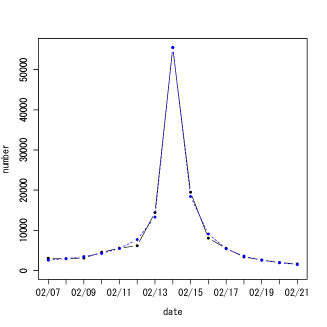
log-likelihood	$95\%$ confidence interval
$\alpha_{b}=3.498$	$3.267<\alpha_{b}<3.728$
$\beta_{b}=0.951$	$0.929<\beta_{b}<0.973$
$\gamma=55538.8$	$54728.4<\gamma<56349.3$
$\alpha_{a}=0.742$	$0.707<\alpha_{a}<0.777$
$\beta_{a}=1.991$	$1.935<\beta_{a}<2.046$

Figure 3: Valentine’s Day 2014 for power-law decay independence model

Based on the power-law decay independence model we considered predicting the after-event parameters based on the data before the event. However this was difficult, because of the asymmetry found in many events. To confirm this phenomenon we performed multiple regression analysis, where the before-event parameters $\alpha_{b},\beta_{b},\gamma$ are explanatory variables and the after-event parameters $\alpha_{a},\beta_{a}$ are objective variables. But we did not find significant correlation.

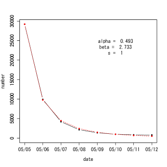
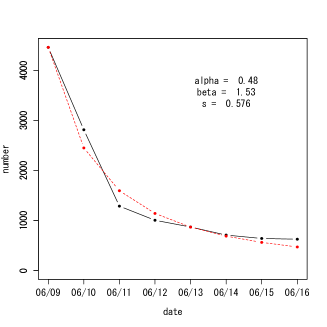
Kodomo no Hi 2014                        Yuko Oshima

Figure 4: Fit of the AR(2) model

4.2 Parameter estimation of the AR(2) model

In Table 3 we show the fit of AR(2) model to our data. In Table 3 “log-lik.” stands for the log-likelihood of the estimated model. Figure 4 shows the fit of the AR(2) model for “Kodomo no Hi” and for “Yuko Oshima” as typical examples. In Figure 4 $s$ is estimated as $s=1$ for “Kodomo no Hi”, whereas $s$ is estimated as $s=0.576$ for “Yuko Oshima”. It seems that the parameter $s$ reflects the property of the event. The parameter $s$ tends to be close to 1 for events with faster decay patterns, but tends to be less than one for events with long-lasting interest after the events. This is reasonable, because $1-s$ represents the effect of two days ago and $s=1$ means that the autocorrelation is fully explained only by the number of postings one day ago. We compared AIC (Akaike’s Information Criterion) for AR(2) model and AIC for AR(2) model with $s=1$. For many data sets AIC was smaller when $s$ is estimated to be less than 1.

4.3 Parameter estimation of the unifying model

In Table 4 we apply the unifying model (6) to data. In the Table 5 we compare the unifying model and other models based on AIC. In many cases the values of the parameters $u,v$ are close to 1 in this model. This suggests that the unifying model is over-parameterized for many events and the maximum likelihood estimation is not very stable. Indeed when we compare AIC for various models, often other models have smaller AIC than the unifying model.

5 Summary and discussion

In this paper we proposed a Poisson autoregression model with the power-law decay of the mean parameter for the number of postings data. Our model shows a good fit to various Japanese social networking data. Also the parameters of our model are easy to interpret and our model is useful in describing patterns of the events. Since the length of the data considered in this paper is fairly short, covering only about one month, the unifying model in (6) with five parameters is probably flexible enough. In fact for many events, we found that smaller models than the unifying model showed better fits.

Our model assumes that there is a single date $t_{0}$ of an event. Some events such as the Olympic games have longer duration. The pattern of number of postings during the event with longer duration seems to be more complicated, although the patterns before the beginning of the event and the after the event seem to be similar to single-day events. It is not clear how to generalize our model to events with a longer duration.

From practical viewpoint, it is important to predict the peak level $\gamma$ of the number of postings and the after-event parameters $\alpha_{a},\beta_{a}$ before the event. However we found that this prediction was difficult for our data. Therefore in data analysis in Section 4, we separately estimated the before-event parameters and the after-event parameters, although for the modeling purpose this is somewhat unsatisfactory. As discussed at the beginning of Section 3 our conditional Poisson regression model is not suited for the prediction before the event. In addition, if the event has some surprising element on the date of the event, then it is naturally difficult to predict it before the event. We could use some characteristic of a particular event for the purpose of prediction. For example, national holiday has a fixed date every year and we can analyze stability of the pattern from year to year.

Table 1: Social networking data in Japan, 2014

Date	ID	Searchword	Remarks
1/13	Seijin	Seijin no Hi	Coming-of-Age Day
1/26	O-Marathon	Osaka International Ladies Marathon
2/3	Setsubun	Setsubun	Bean Throwing Night
2/8	Sochi	Sochi Olympics	The opening ceremony took place February 7, local time.
2/9	Uemura	Aiko Uemura	The women’s moguls final
2/11	Kenkoku	Kenkokukinenbi	National Foundation Day
2/14	Valentine	Valentine’s Day
2/15	Hanyu	Yuzuru Hanyu	Figure skating men’s singles free
2/16	Kasai	Noriaki Kasai	Large hill individual men final
2/21	Asada	Mao Asada	Figure skating ladies’s singles free
2/23	T-Marathon	Tokyo Marathon
3/3	Academy	Academy Awards	The Oscar ceremonies took place March 2, local time.
3/11	Earthquake	The Great East Japan Earthquake
3/14	White	White Day
3/21	Shunbun	Shunbun no Hi	Vernal Equinox Day
3/24	mayoral	Osaka’s mayoral elections
5/5	Kodomo	Kodomo no Hi	Children’s Day
6/9	Oshima	Yuko Oshima	AKB graduation performance
6/15	W-cup	The World Cup	In Japan’s opening match against Cote d’Ivoire
6/21	Geshi	Geshi	the summer solstice

Table 2: Parameter estimation of the power-law decay independence model

ID	$\alpha_{b}$	$\beta_{b}$	$\gamma$	$\alpha_{a}$	$\beta_{a}$
Seijin	0.889	1.493	53664	0.908	1.463
O-Marathon	7.902	0.858	993	0.207	4.337
Setsubun	2.694	1.318	105334	0.397	2.921
Sochi	0.179	5.499	5479	1.089	1.65
Uemura	0.346	3.256	4992	0.231	3.436
Kenkoku	1.405	2.012	7708	1.021	2.122
Valentine	3.498	0.951	55539	0.742	1.991
Hanyu	0.898	1.823	10317	2.353	0.891
Kasai	599789.772	0.221	3368	0.131	4.584
Asada	0.447	2.755	18898	1.289	1.047
T-Marathon	2.327	1.186	8702	0.619	1.948
Academy	39.489	0.423	2923	3.97	0.302
Earthquake	10.695	0.822	41580	2.611	1.185
White	6.285	0.691	45488	0.309	2.483
Shunbun	2.99	1.259	14379	0.902	1.969
Mayoral	0.096	7.803	1632	1.217	1.375
Kodomo	14.37	0.783	29200	0.637	2.316
Oshima	1.083	1.136	4456	0.673	1.23
Wcup	0.013	34.707	45925	1.091	0.787
Geshi	8.096	0.746	8183	0.766	1.498

Table 3: Parameter estimation of the AR(2) model

	AR(2) model						$s=1$
ID	$\alpha$	$\beta$	$\gamma$	$s$	log-lik.	AIC	log-lik.	AIC
Seijin	0.612	1.834	53188	1.000	-342.303	690.606	-342.303	688.606
O-Marathon	0.105	7.517	992	0.810	-58.919	123.839	-59.298	122.597
Setsubun	0.265	3.944	105410	0.621	-2498.205	5002.410	-2617.576	5239.152
Sochi	0.946	1.774	5374	0.671	-39.372	84.743	-39.575	83.150
Uemura	0.276	3.173	5348	0.361	-89.743	185.485	-105.474	214.949
Kenkoku	0.688	2.720	7679	1.000	-58.690	123.380	-58.690	121.380
Valentine	0.722	2.040	55456	0.057	-154.633	315.266	-262.679	529.358
Hanyu	1.919	0.951	9969	0.957	-82.052	170.104	-82.115	168.231
Kasai	0.097	5.667	3381	0.227	-185.319	376.637	-246.634	497.269
Asada	1.486	0.984	18939	0.341	-135.275	276.551	-181.722	367.444
T-Marathon	0.331	2.934	8688	1.000	-185.955	377.911	-185.955	375.911
Academy	0.692	0.743	2923	1.000	-958.221	1922.442	-958.221	1920.442
Earthquake	2.615	1.207	41566	0.054	-298.935	603.871	-739.180	1482.360
White	0.313	2.485	45438	0.131	-268.771	543.542	-459.159	922.317
Shunbun	1.030	1.821	14369	0.405	-64.870	135.740	-73.371	150.742
Mayoral	1.175	1.385	1581	0.342	-43.581	93.163	-49.383	102.766
Kodomo	0.493	2.733	29201	1.000	-104.649	215.298	-104.649	213.298
Oshima	0.480	1.530	4458	0.576	-155.904	317.808	-167.602	339.205
Wcup	0.930	0.859	44480	0.666	-1994.083	3994.167	-2142.728	4289.457
Geshi	0.552	1.789	8174	1.000	-140.557	287.115	-140.557	285.115

Table 4: Parameter estimation of the unifying model

ID	$\alpha$	$\beta$	$\gamma$	$w$	$u$	$v$	log-lik.	AIC
seijin	0.735	1.618	53188	0.643	0	1	-329.506	669.013
O-Marathon	0.177	4.857	992	0.287	0.005	0.996	-53.204	116.407
Setsubun	0.398	2.919	105410	0.998	0.999	0.999	-2092.256	4194.512
Sochi	1.053	1.665	5374	1	1	1	-37.463	84.927
Uemura	0.286	3.055	5348	1	1	1	-68.389	146.779
Kenkoku	0.817	2.404	7679	0.670	0	1	-58.269	126.538
Valentine	0.741	1.993	55456	0.007	0.988	0.561	-145.248	300.495
Hanyu	2.168	0.901	9969	0.993	0.702	0.996	-71.639	153.279
Kasai	0.135	4.488	3381	0	0.966	0.999	-138.561	287.121
Asada	1.296	1.045	18939	0	1	1	-109.559	229.119
T-Marathon	0.433	2.388	8688	0.674	0.002	0.995	-180.467	370.934
Academy	4.524	0.288	2923	0.977	0.920	0.990	-604.371	1218.743
Earthquake	2.710	1.173	41566	0.429	1	0	-277.531	565.061
White	0.310	2.475	45438	0.010	0.997	0.873	-220.389	450.779
Shunbun	0.901	1.969	14369	0	1	1	-59.885	129.770
Mayoral	1.145	1.396	1581	0	1	1	-37.753	85.506
Kodomo	0.493	2.733	29201	1	0	1	-104.649	219.298
Oshima	0.674	1.229	4458	1	1	1	-120.807	251.614
Ｗcup	0.966	0.815	44480	0	1	1	-1249.637	2509.273
Geshi	0.632	1.619	8174	0.814	0	1	-137.969	285.939

Table 5: Comparison of models based on AIC

		$w=1$
				$u=1$	$u=0$
ID	AIC	$u$	AIC	AIC	AIC
Seijin	669.013	0.39	667.378	732.505	688.606
O-Marathon	116.407	0.764	112.277	111.576	122.597
Setsubun	4194.512	1	4190.483	4188.482	5239.152
Sochi	84.927	1	80.927	78.927	83.15
Uemura	146.779	1	142.777	140.777	214.949
Kenkoku	126.538	0.334	122.515	127.391	121.38
Valentaine	300.495	1	311.419	309.419	529.358
Hanyu	153.279	0.705	149.28	150.843	168.231
Kasai	287.121	1	283.097	281.095	497.269
Asada	229.119	1	225.119	223.119	367.444
T-Marathon	370.934	0.41	364.891	394.555	375.911
Academy	1218.743	0.905	1212.032	1217.415	1920.442
Earthquake	565.061	1	644.564	642.564	1482.36
White	450.779	1	449.023	447.023	922.317
Shunbun	129.77	1	125.77	123.77	150.742
Mayoral	85.506	1	81.506	79.506	102.766
Kodomo	219.298	0	215.298	273.882	213.298
Oshima	251.614	1	247.613	245.613	339.205
Ｗcup	2509.273	1	2505.273	2503.273	4289.457
Geshi	285.939	0.211	282.618	357.08	285.115

References

- [1] Valentina Alfi, Andrea Gabrielli and Luciano Pietronero. How people react to a deadline: time distribution of conference registrations and fee payments. Central European Journal of Physics, 7, No.3, 483–489, 2009.
- [2] Sitaram Asur, Bernardo A. Huberman, Gábor Szabó and Chunyan Wang. Trends in Social Media : Persistence and Decay. In Proceedings of CoRR. pp.434–437. 2011.
- [3] Patrick T. Brandt and John T. Williams. A linear Poisson autoregressive model: the Poisson AR() Model. Political Analysis, 9, Issue 2, 164–184, 2001.
- [4] Trevor Fenner, Mark Levene and George Loizou. A bi-logistic growth model for conference registration with an early bird deadline. Central European Journal of Physics, 11, No.7, 904–909, 2013.
- [5] Konstantinos Fokianos. Count time series models. in Time Series Analysis: Methods and Applications, Handbook of Statistics, Vol.30, (ed. T.S.Rao, S.S.Rao and C.R.Rao), North Holland, Amsterdam, 315–347, 2012.
- [6] Konstantinos Fokianos, Anders Rahbek, and Dag Tjøstheim. Poisson autoregression. Journal of the American Statistical Association, 104, 1430-1439, 2009.
- [7] Konstantinos Fokianos. Some recent progress in count time series. Statistics, 45, 49–58, 2011.
- [8] R. K. Freeland and B. P. M. McCabe. Analysis of low count time series data by Poisson autoregression, Journal of Time Series Analysis, 25, Issue 5, 701–722, 2004.
- [9] Akshay Java, Xiaodan Song, Tim Finin and Belle Tseng. Why we twitter: understanding microblogging usage and communities, in Proceedings of Joint 9th WEBKDD and 1st SNA-KDD Workshop ’07, pp.56–65, 207.
- [10] Yukie Sano, Kenta Yamada, Hayafumi Watanabe, Hideki Takayasu and Misako Takayasu. Empirical analysis of collective human behavior for extraordinary events in the blogosphere, Physical Review E, 87, 012805, 2013.
- [11] Takeaki Sakaki, Makoto Okazaki and Yutaka Matsuo. Earthquake shakes Twitter users: real-time event detection by social sensors. In Proceedings WWW ’10, pp.851–860. 2010.
- [12] Amanda L. Traud, Peter J. Muchaa and Mason A. Porter. Social structure of Facebook networks. Physica A, 391, 4165–4180, 2012.
- [13] Fukang Zhu. Modeling overdispersed or underdispersed count data with generalized Poisson integer-valued GARCH models. Journal of Mathematical Analysis and Applications, 389, 58–71, 2012.