A novel quantum-mechanical interpretation of the Dirac equation
Abstract
A novel interpretation is given of Dirac’s “wave equation for the relativistic electron” as a quantum-mechanical one-particle equation. In this interpretation the electron and the positron are merely the two different “topological spin” states of a single more fundamental particle, not distinct particles in their own right. The new interpretation is backed up by the existence of such “bi-particle” structures in general relativity, in particular the ring singularity present in any spacelike section of the spacetime singularity of the maximal-analytically extended, topologically non-trivial, electromagnetic Kerr–Newman spacetime in the zero-gravity limit (here, “zero-gravity” means the limit , where is Newton’s constant of universal gravitation). This novel interpretation resolves the dilemma that Dirac’s wave equation seems to be capable of describing both the electron and the positron in “external” fields in many relevant situations, while the bi-spinorial wave function has only a single position variable in its argument, not two — as it should if it were a quantum-mechanical two-particle wave equation. A Dirac equation is formulated for such a ring-like bi-particle which interacts with a static point charge located elsewhere in the topologically non-trivial physical space associated with the moving ring particle, the motion being governed by a de Broglie–Bohm type law extracted from the Dirac equation. As an application, the pertinent general-relativistic zero-gravity Hydrogen problem is studied in the usual Born–Oppenheimer approximation. Its spectral results suggest that the zero- Kerr–Newman magnetic moment be identified with the so-called “anomalous magnetic moment of the physical electron,” not with the Bohr magneton, so that the ring radius is only a tiny fraction of the electron’s reduced Compton wavelength.
©2014/2015. The authors. Reproduction for non-commercial purposes is permitted.
email: miki@math.rutgers.edu, shadi@math.rutgers.edu
1 Introduction
We begin with a brief history of Dirac’s equation and its quantum mechanical interpretations. Readers who are familiar with this subject may wish to skip ahead to section 1.2 for an introduction to our novel proposal, and for an executive summary of our main results at the end of that section.
1.1 Quest for the quantum-mechanical interpretation of Dirac’s equation
Many textbooks and monographs (e.g. [60], [40], [81], [70]) tell the story of Dirac’s marvelous discovery of the special-relativistic generalization of Pauli’s non-relativistic spinor wave equation for the “spinning electron”: his ingenious insight that a first-order partial differential operator is needed rather than the second-order wave operator in the so-called111We are alluding to the history of this equation: first contemplated by Schrödinger before he discovered his nonrelativistic equation, and rediscovered by various physicists, amongst them Klein, Gordon, and also Pauli. Klein–Gordon equation; his equally ingenious insight that complex four-component bi-spinors, instead of Pauli’s complex two-component spinors, are needed to accomplish this goal; his consequential formulation of the equation and his skillful analysis of the same; the -factor 2; the explicit solution of the Hydrogen problem in terms of elementary functions (by Darwin [24] and Gordon [39]), and the surprising exact agreement of the Dirac point spectrum with Sommerfeld’s fine structure formula (save the labeling of the energy and angular momentum levels);222For a modernized semi-classical Bohr–Sommerfeld approach that leads to the correct labeling, see [49]. the strange occurrence of a negative energy continuum below (with the electron’s rest mass, and the speed of light in vacuum), leading to Dirac’s ultimate triumph: the prediction of the existence of the anti-electron (a.k.a. positron) — based on his “holes in the Dirac sea” interpretation.
Yet, not all is well. The most perplexing (and intriguing) part of the above success story is that it is based on Dirac’s changing the rules of the game while he was playing it. Thus, originally formulating it as a quantum-mechanical one-particle wave equation on one-particle configuration space, Dirac — by postulating that all negative energy continuum states are occupied with electrons — switched to an infinitely-many particle interpretation on physical space: a “poor man’s quantum field theory” (yet an important stepping stone towards quantum electrodynamics, one that still is the subject of serious studies by mathematical physicists [58]). And while it is difficult to argue with practical success, Dirac’s ad-hoc “holes in the negative energy sea” theory can be criticized for de-facto bypassing the conceptual problem of the proper quantum-mechanical interpretation of Dirac’s equation (assuming there exists one!), rather than addressing it.
Stückelberg [73] and Feynman [34] revived the quantum-mechanical interpretation of Dirac’s equation and argued that it is an equation for both, the electron and the positron, cf. Thaller [80]: “[U]p to now no particular quantum mechanical interpretation [of Dirac’s wave equation] is generally accepted. … [T]he Stückelberg–Feynman interpretation (Stückelberg 1942, Feynman 1949) … is intermediate between a one-particle theory and Dirac’s hole theory, because it claims that the Dirac equation is able to describe two kinds of particles, namely electrons and positrons (but not their interaction; negative energy states are directly observed as positrons with positive energy).” Thaller, who adopts the Stückelberg–Feynman interpretation in his scattering theory, goes on to emphasize that it is “formulated in the language of wave packets … and does not rely on unobservable objects like the Dirac sea.” In a nutshell, the main idea is that wave packets composed of only positive energy eigenfunctions and scattering states “describe” electrons, those composed of only negative energy eigenfunctions and scattering states “describe” positrons; cf. also [16]. The problem with identifying electrons and positrons with respect to the respective subspaces of the “free” Hamiltonian is that switching on “external” fields may induce transitions between the two; or, in mathematical language: the positive and negative energy Hilbert subspaces for the free Hamiltonian may not be invariant under the unitary evolution of a scattering problem. Klein’s paradox (see [81]) shows that these subspaces are not always invariant under the unitary evolution, indeed. Furthermore there are examples of physically interesting electric potentials (e.g. a regularized Coulomb potential) which can generate negative energy eigenstates which clearly are to be interpreted as belonging to the electron, not the positron; see [40]. Even in favorable situations, mixed initial conditions can pose an interpretational dilemma.
Thus not all is well with the Stückelberg–Feynman interpretation either. To Thaller’s emphasis of its limitations we here add another troublesome criticism, namely that this interpretation is in conflict with established quantum-mechanical many-body concepts. Thus, while Dirac’s bi-spinorial wave function depends (beside time) only on one position variable, it should have two position variables in its arguments, not merely one, if Dirac’s equation truly were a quantum-mechanical two-particle equation. For then it has to reproduce Pauli’s quantum-mechanical two-particle equation for a non-relativistic electron–positron pair in the non-relativistic limit, and this Pauli equation — which is the traditional starting point for computing the leading-order spectral properties of positronium, with relativistic corrections computed perturbatively subsequently [4] — does have a complex four-component wave function with two position variables in its arguments.333There is one loose end in this argument — which can easily be tied up. More to the point, as in the quantum-mechanical analog of the Kepler problem, one can change coordinates from the two particle position vectors (defined w.r.t. some inert fixed point) to center-of-mass coordinates (w.r.t. the same fixed point) plus relative coordinates. In the spinless non-relativistic limit the center-of-mass coordinates can be factored out, and the remaining wave equation in the relative coordinates is effectively a one-body equation for a test particle in an external Coulomb field. So one may speculate whether Dirac’s equation is perhaps of this type, describing the relative motion of electron and positron in relative coordinates. Unfortunately the mass parameter in Dirac’s equation “for the relativistic electron” is a factor 2 too big for this interpretation to be feasible, putting to rest speculations in this direction.
1.2 A novel proposal
Since the enigmatic quantum-mechanical character of “Dirac’s equation for the electron” manifests itself in the seemingly contradictory aspects that, on one hand, it has all the formal hallmarks of a single-particle equation, while, on the other, its set of solutions covers (much of) the physics of both the electron and the anti-electron, the only logical conclusion that avoids this paradox is that electron and anti-electron are not separate entities but merely “two different sides of the same medal.” By this we do not mean the well-known charge-conjugation transformation which maps a “negative-energy Dirac electron state” into a “positive-energy Dirac positron state,” and vice versa; neither do we mean the interpretation suggested by Stückelberg, Wheeler, and Feynman that an “electron moving backward in time appears as a positron moving forward in time.” Rather, we propose that electron and anti-electron are two different “topological-spin” states of a single, more structured particle (moving forward in time).
Our novel interpretation is backed up by the fact that such bi-particle structures exist in some electromagnetic spacetime solutions of Einstein’s classical theory of general relativity.444By invoking a classical physical theory, in our case Einstein’s general relativity, we are simply following the standard protocol of “first quantization.” Enjoying the benefit of hindsight we may simplify our task and look for the desired electromagnetic “bi-particle structure” in classical physical theory, then compute its electromagnetic interaction with some other classical elecromagnetic object, in particular a point charge. This classical interaction then enters the pertinent quantum-mechanical wave equation obtained from “first quantization,” in our case Dirac’s equation. The remaining task then is to show that this Dirac equation makes the right physical predictions and avoids any of the paradoxical aspects that we have discussed. More concretely, we mean the structure commonly known as the “ring555What is “ring-like” is actually a constant- “snapshot” of the spacetime singularity. singularity” of the maximal-analytically extended, topologically non-trivial,666The complement of a wedding ring in three-dimensional Euclidean space is topologically non-trivial, too, but “looping through the ring once brings you back to where you began;” in a spacelike slice of the maximal-analytically extended Kerr–Newman spacetime “you need to loop through the ring twice to get back to square one.” electromagnetic spacetime of Newman et al. [64, 14] — in its zero-gravity limit. Here, “zero-gravity limit” means the limit , where is Newton’s constant of universal gravitation, applied to the Kerr–Newman metric777A priori speaking the limit should also be applied to the expressions for the Kerr–Newman electromagnetic fields, but these are -independent in the coordinates we use. expressed in any one of the most symmetric global coordinate charts.
1.2.1 The zero-gravity Kerr–Newman (zKN) spacetime.
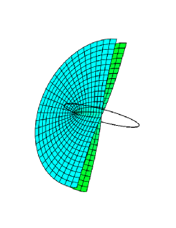
As shown rigorously in an accompanying paper [77], this zKN spacetime itself is a flat but topologically nontrivial solution of the vacuum Einstein equations , while its electromagnetic fields are static Appell–Sommerfeld solutions888Remarkably, the electromagnetic fields were discovered in 1887 by Appell [1] by performing a complex translation “of physical space” in the Coulomb potential. However, Appell did not realize, apparently, that the complex generalization of the Coulomb potential lives on a topologically non-trivial extension of Euclidean . This insight is due to Sommerfeld [71], who is credited with introducing the concept of branched Riemann space, a three-dimensional analog of a Riemann surface, on which multi-valued harmonic functions such as the Appell fields become single-valued. of the linear Maxwell equations on this spacetime, with well-behaved sesqui-pole sources concentrated on its spacelike ring singularity. Most importantly, the ring singularity of a spacelike snapshot of the spacetime appears to be positively charged in one “sheet,” yet negatively charged in the other, with pertinent electric monopole asymptotics near spacelike infinity (see Fig. 1); analogous statements hold for the magnetic structure, with dipole asymptotics near spacelike infinity. The electromagnetically anti-symmetric spacelike ring singularity of this double-sheeted Sommerfeld space is precisely the kind of bi-particle-like structure which vindicates our informal wording that “electron and anti-electron are two sides of one and the same medal” as mathematically realized in a classical physical field theory, and therefore as putatively physically viable in a quantized theory.

We stress the importance of the zero-gravity limit of the maximal-analytically extended Kerr–Newman spacetime and its elecromagnetic fields [77] for getting our electron/anti-electron bi-particle interpretation of its ring singularity off the ground. The reason is that the energy-momentum-stress tensor of the electromagnetic Appell–Sommerfeld fields is not locally integrable at the ring singularity, so when coupled to spacetime curvature by “switching on gravity,” it produces the physically “pathological” effects of the maximal-analytically extended Kerr–Newman spacetime (such as closed timelike loops; the const. ring singularity itself is also timelike when and not interpretable as a stationary particle-like source [19])999While “switching off gravity” should not be viewed as a troublesome step, our statement that the zero- limit is important to get our electron/anti-electron bi-particle interpretation of its ring singularity off the ground, in the sense that the KN “ring singularity” cannot be given a bi-particle interpretation for , could seem to deal a fatal blow to our proposal. However, the problems we have in mind are similar to those affecting the usual textbook formulation of Dirac Hydrogen, viz. “Dirac’s equation for a point (test) electron in the field of a point proton at rest in Minkowski spacetime” — as soon as one “switches on ” to compute the general-relativistic corrections to the Sommerfeld spectrum from eigenstates for Dirac’s equation of a point (test) electron in the Reissner–Nordström spacetime, “all hell breaks lose” (see [54] for a review). The reason is once again the local non-integrability of the energy-momentum-stress tensor of the classical electromagnetic field, which in the usual textbook case is the field of a point charge. This clearly suggests that the culprit is Maxwell’s linear vacuum field equations, and that replacing them with non-linear field equations that produce an integrable energy-momentum-stress tensor, the pathologies might go away and general-relativistic gravitational curvature corrections to the spectral features of special-relativistic Dirac Hydrogen may eventually come out not larger than the tiny Newtonian gravitational effects relative to the electromagnetic effects on the non-relativistic Schrödinger spectrum of Hydrogen. More about this in our concluding section. In short, the pathological problems of the Kerr–Newman singularity are bad news for the physical interpretation of the maximal-analytically extended Kerr–Newman spacetime with , but not bad news for our proposal that electron and anti-electron might be the two electromagnetic “sides” of a bi-particle-like ring singularity associated with a two-sheeted space. — more on this in section 2. The limit removes all these troublesome features of the Kerr–Newman spacetime while retaining the topological and electromagnetic features that can be given a clear physical meaning.101010It is our pleasant duty to note here that we are not the first to try to associate the double sheetedness of the zKN spacetime and its anti-symmetric electromagnetism with particle / anti-particle symmetry. Namely, after reading an earlier version of our paper, Prof. Ted Newman kindly send us a letter with (amongst other valuable information) the following historical note: “I had (in about 1966) myself noted — in the limit — that by going along the axis of symmetry from large down to zero and then to negative that the sign of the charge would change. Kerr and Penrose did clarify this for me. I and one of my Polish colleagues, spent a great deal of time — talking and trying out ideas concerning the double sheetedness — mainly trying to put it into the context of parity, time reversal and charge conjugation symmetry. It was a very enticing idea. Unfortunately we never could make it into a unified theory or even a coherent idea. We eventually gave it up — not because it was wrong — but because we were stuck and could not make it work.” In this paper we will see that the double sheetedness and its charge (anti-)symmetry are associated not with parity, time reversal, and charge conjugation symmetry operations, but with a novel symmetry operation on the Dirac bi-spinor, associated with what we call “topo(logical)-spin” of the zKN ring singularity, viz. the particle/anti-particle symmetry of the zKN ring singularity is implemented in a topo-spin flip operation and, thus, is somewhat akin to Heisenberg’s iso-spin concept for nucleons.
1.2.2 The physical spacetime of a moving zKN-type ring singularity.
Having identified a candidate structure for our electron/anti-electron bi-particle proposal in form of the ring singularity of a snapshot of the static zKN spacetime, we next describe the physical spacetime associated with such a ring-like bi-particle when moving, were motion is understood as relative to an inertial frame attached to an arbitrarily chosen origin (the analog of Carl Neumann’s “ body frame” for Newton’s mechanics). We restrict our considerations mostly to the quasi-static motions approximation and only briefly comment on more general motions.
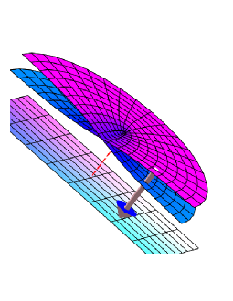
In the simplest special case, when the ring particle is at rest relative to the frame, the spacetime is simply (a spacelike translation and rotation of) the static zKN spacetime, of course. Furthermore, a Lorentz boost of such a static zKN spacetime coordinates produces the spacetime of a ring singularity in straight inert motion relative to the frame; see Fig. 2 for a totally stripped down illustration of the physical spacetime with a ring singularity in straight motion contrasted with the corresponding illustration of a test particle in straight motion in the zKN spacetime.

Note that the ring will be circular generally only in its rest frame, whereas a Lorentz boost will render it generally elliptical. However, neglecting effects of order as relatively small in the quasi-static motions approximation, a moving ring can be described as circular to leading order.
The physical spacetime with a single moving space-like ring singularity is generally not obtained by a Lorentz boost of zKN, but in the quasi-static approximation it is foliated by constant-time Sommerfeld spaces which are all snapshots of the zKN spacetime with a ring singularity translated and rotated relative to the fixed frame. Unfortunately, it’s not so easy to generalize the left illustration in Fig. 2 to visualize a double sheeted spacetime with a ring singularity not moving in a straight line motion with respect to an point having a vertical world line. Yet, we hope that the general idea of what this physical spacetime is has become clear.
Incidentally, the double-sheeted physical zero- spacetime with a generally moving ring-like singularity will feature snapshots having deformed ring singularities, and a proper treatment would presumably require solving the so-called vacuum Einstein equations. It is likely that the spacetime will then also feature “gravitational” waves.111111Note that uncouples the spacetime structure from its matter and field content, but the spacetime metric does not need to be flat. In particular, it can feature wave-like disturbances propagating at the speed of “light.”
1.2.3 The configuration space(time) of a moving zKN-type ring singularity.
Finally, to formulate Dirac’s equation for the spinor wave function of such a ring-like bi-particle we need to identify the configuration space of a single ring particle on which the wave function is defined (as bispinor-valued function), and this is simply the space of all possible cofigurations for the particle relative to the frame. In case of the ring singularity, classically knowing its configuration means knowing the location of the center of the ring as well its orientation, i.e. the unit normal to the plane of the ring. Quantum mechanically however, this orientation vector is itself determined by a bi-spinor wave function (as we will show), so that specifying the location of the center of the ring, with respect to a frame attached to the point of the space, should suffice. It follows that the configuration space for a ring-like particle should also be double-sheeted, since one can contemplate the origin to be “swallowed” by the ring as its center moves, causing the origin to end up on a different sheet of the physical space. Since that is a different configuration for the ring, one sheet will not be enough to encode all the possible positions of the center of the ring; thus the configuration space is also double-sheeted, and in fact isomorphic to the Sommerfeld space obtained by a constant-time snapshot of the zKN spacetime as one can easily show. We remark that formally the Dirac equation for a quasi-statically moving ring singularity is therefore a bispinor-valued wave equation on the configuration spacetime which is isomorphic to zKN. It is important not to confuse this configuration spacetime with a physical zKN spacetime, though.
1.2.4 Enter Dirac’s equation.
To test our bi-particle interpretation of the ring singularity of the constant-time snapshot of the maximal-analytically extended zKN spacetime as an electron/anti-electron structure whose motion relative to an frame is governed by Dirac’s equation we study the pertinent general-relativistic zero-gravity Hydrogen problem in the usual Born–Oppenheimer approximation. We first show that the classical electromagnetic interaction of a static zKN ring singularity with a point charge located at the point in the static spacelike slice of zKN is given by the minimal coupling formula used to describe the interaction of a test point charge in the field of a given zKN singularity — to avoid confusion with the “naive minimal coupling” evaluation of the Coulomb field of the point charge at the center of the zKN ring singularity (times its charge parameter), we will call our interaction formula a “minimal re-coupling” term. Next we show that although the zKN singularity is not point- but ring-like, in the quasi-static motions regime one and the same Dirac equation covers these two interpretations of the “point charge plus zKN ring singularity” system (i.e., only the narrative changes); in particular, the eigenstates are captured correctly. In another accompanying paper [53] we have rigorously studied this Dirac equation (in the interpretation “test point charge in the zKN spacetime”), and in the present paper the results of [53] will be explained in the novel interpretation put forward here. In addition, here we will argue — compellingly as we believe — that our spectral results suggest as choice for the ring diameter of the electron/anti-electron bi-particle structure not the reduced Compton wavelength of the electron, , as proposed in earlier, different studies which aimed at linking the Kerr–Newman spacetime with Dirac’s electron (see Appendix C), but only a tiny fraction of it.
Lastly, we will show that with the help of the Dirac bi-spinors de Broglie–Bohm type laws of motion and orientation can be formulated for the zKN ring singularity in the quasi-static regime.
1.2.5 Summary.
In this paper we propose a fundamentally new quantum-mechanical interpretation of Dirac’s equation as a single-particle equation for a fermionic elementary particle which is both an electron and an anti-electron. We
-
•
argue that the primitive ontology of such a bi-particle which is both an electron and a positron is realized by the general-relativistic electromagnetic ring singularity of a constant-time snapshot of the double-sheeted zero-gravity Kerr–Newman (zKN) spacetime;
-
•
explain that the physical spacetime of such a ring-like bi-particle in quasi-static motion with respect to a rest frame attached to an arbitrarily chosen origin (Neumann’s point) is a two-sheeted spacetime with a “wiggly” timelike tubular region traced out by the moving ring singularity, such that every constant-time snapshot (w.r.t. the frame) is a combined translation and rotation of the constant-time snapshot of the zKN spacetime;
-
•
explain that the configuration spacetime of this ring-like bi-particle in quasi-static motion is isomorphic to the zKN spacetime — any point in the pertinent configuration space represents a possible position of the center of the ring singularity, relative to the frame;
-
•
show that a sheet swap in configuration space is associated with a topological spin operator acting on the bi-spinorial wave function defined on configuration space;
-
•
show how the bi-spinorial wave function on configuration space naturally defines a three-frame attached to the center of the ring singularity, and thereby an orientation (spin) vector;
-
•
formulate quantum laws of motion for the center and orientation of this two-faced particle using the de Broglie–Bohm approach relative to the frame, involving a bi-spinorial wave function satisfying Dirac’s equation on the configurational zKN spacetime;
-
•
compute the classical electromagnetic interaction in physical space of a quasi-static ring singularity with an infinitely massive point charge (modeling a proton) located at the point, showing it is identical to the minimal coupling formula of a point charge in the electromagnetic Appell–Sommerfeld (viz. zKN) fields;
-
•
explain that the Dirac spectrum in our model coincides with the spectrum of a “Dirac point positron” in a given, fixed background zKN spacetime — we then invoke the results we have previously obtained in this test-charge situation, namely: the self-adjoineness of the Dirac Hamiltonian, the symmetry of its spectrum about 0, the essential spectrum being , and the existence of discrete spectrum under suitable smallness assumptions;
-
•
argue that the discrete spectrum reproduces the Sommerfeld fine structure formula (in fact, a positive and a negative copy of it) in the limit of vanishing ring radius, and that the magnitude of effects like hyperfine structure and Lamb(-like) shift of the spectral lines put a limit on the size of the ring singularity which corresponds to the identification of the zKN magnetic moment with the anomalous magnetic moment of the electron.
1.3 The structure of the ensuing sections
In section 2 we summarize the basic formulas of the zKN spacetimes and their electromagnetic fields, and also some straightforward generalizations of the latter. This material is taken from [77].
Section 3: We formulate the Dirac equation for a zKN-type ring singularity that interacts with an infinitely massive static point charge located at the point in this topologically non-trivial (double-sheeted) manifold. We vindicate the “minimal re-coupling” interaction formula introduced here. We then summarize the pertinent results obtained in [53] for the equivalent Dirac problem of a test point positron in the field of an infinitely massive zKN singularity: essential self-adjointness of the Hamiltonian; symmetry of its spectrum about zero; the usual Dirac continuum with a gap; a discrete spectrum inside the gap if the ring radius and the coupling constant are small enough — in principle numerically computable by ODE methods using the Chandrasekhar–Page–Toop separation-of-variables method in concert with the Prüfer transform. Here, we also show (formally) that in the limit of vanishing diameter of the ring singularity the positive part of the discrete spectrum reproduces Sommerfeld’s fine structure spectrum (with correct Dirac labeling) for Born–Oppenheimer Hydrogen, while the negative part produces the negative of the same (we also explain why the familiar special-relativistic Dirac spectrum only contains half of it). We argue why this result implies that the choice of ring diameter for an electron/anti-electron bi-particle structure should only be a tiny fraction of the reduced Compton wavelength of the electron. We also explain why a study of finite-size effects of the ring singularity on the spectrum using perturbation theory may be problematic, while perturbative computations of effects of a Kerr–Newman-anomalous magnetic moment on the spectrum is presumably feasible. The technical sections 3.3.2, 3.4.1, 3.4.2 are nearly verbatim adapted from [53] and reproduced here for the convenience of the reader.
Section 4: We formulate de Broglie–Bohm laws of motion and orientation for the zKN-type ring singularity.
Section 5: We conclude with suggesting future work. In particular, we include some speculations about the proper two- and many-body theories consisting entirely of (semi-classically) electromagnetically interacting zKN ring singularities. The two-body problem is clearly of interest as a putative model for positronium, while the many-body theory may offer an intriguing novel explanation of why the particle/anti-particle symmetry is broken in our (part of the) universe.
Appendix: Two appendices supply technical material, one appendix contrasts our work with earlier proposals to link the Kerr–Newman spacetime with “Dirac’s equation for the electron.”
Almost everywhere in this paper we work in spacetime units in which the speed of light in vacuo , and in the more mathematical parts we will also set , Planck’s constant divided by , equal to unity; in some physically important formulas we will re-instate both and .
2 zKN spacetimes electromagnetic fields, and generalizations
2.1 Electromagnetic spacetimes
An electromagnetic spacetime is a triple , consisting of a four-dimensional manifold , a Lorentzian metric on (here with signature in line with recent mathematical works on the general-relativistic Dirac equation), and a two-form representing an electromagnetic field defined on , altogether solving the Einstein–Maxwell equations (in units in which )
| (1) | |||||
| (2) |
Here, denotes the components of the Ricci curvature tensor and the scalar curvature of the metric . Finally, are the components of the trace-free electromagnetic energy(-density)-momentum(-density)-stress tensor:
| (3) |
where denotes the Hodge duality map. Since is trace-free, viz. , the Ricci scalar , so that (1) simplifies to
| (4) |
2.2 A brief recap of the electromagnetic Kerr–Newman spacetimes
The “outer” Kerr–Newman (KN for short) family of spacetimes is a three-parameter family of stationary axisymmetric solutions to the Einstein–Maxwell equations. The three parameters mentioned are the ADM mass (total energy) m, ADM angular momentum per unit mass , and total charge q; here, ADM stands for Arnowitt, Deser, and Misner, who defined these quantities in terms of surface integrals at spatial infinity; the charge is similarly defined using Gauss’ theorem. Of course, the solution also depends on , though only in combination with m and . The KN metric is singular on the timelike cylindrical surface whose cross-section at any fixed is a circle of (Euclidean) radius , where , and is Newton’s constant of universal gravitation. This circle is commonly referred to as the “ring” singularity. The KN electromagnetic field is also singular on the same ring as the metric, while asymptotically (near spatial infinity) it becomes indistinguishable from an electric monopole field of moment q and a magnetic dipole field of moment in Minkowski spacetime.
The causal structure of the maximal-analytical extension of the KN spacetime is quite complex [19] (see also [42, 65]), and depends on the relationship between the parameters: For (the subextremal case) there is an “ergosphere” region, where due to frame dragging the spacetime is no longer stationary. In addition, there are two horizons. One is an event horizon (boundary of a black hole region) shielding one asymptotically flat end of the manifold from the ring singularity and the acausal region surrounding the latter, and the other a Cauchy horizon, beyond which the initial data do not determine the evolution. For (the superextremal case) there is still an ergosphere region but there is no event horizon, and thus the ring singularity is naked. The region near the ring is particularly pathological in both sub- and super-extremal cases since it includes closed timelike loops. In the superextremal case the presence of these loops turns the entire manifold into a causally vicious set.
2.3 Zero- limit of Kerr–Newman spacetimes and their electromagnetic fields
It is however possible to rid the KN family from all its causal pathologies mentioned above: take the limit of the KN family in a global chart of asymptotically flat coordinates which respect all the symmetries of the spacetime, while fixing the values of the three parameters m,q, and . Since m occurs only in the combination , a two-parameter family of spacetimes, depending on and q, emerges in the limit, and is denoted as the zero- Kerr–Newman (zKN) family. In the zKN family there are no horizons, no ergosphere regions, no closed timelike loops, and no causally vicious regions. Even though the metrics and fields in this family are still singular on a ring (now of radius ), the spacetimes do not suffer from any of these maladies. Indeed, the manifold is locally flat, and the singularity of the metric at a point on the ring is relatively mild, namely conical.
A key feature associated with this ring singularity which survives the zero- limit is the Zipoy topology of the double-sheeted maximal-analytical extension of the KN family of spacetimes. Remarkably, the entire zKN spacetime can nevertheless be covered by a single chart of coordinates, named after Boyer–Lindquist (BL) and usually denoted by , where the timelike coordinate and the spacelike coordinate are Killing parameters (i.e. is a timelike and a spacelike Killing field) and are oblate spheroidal coordinates in const. slices; see Fig. 3. Each constant- slice consists of two copies of (the sheets) that are cross-linked through two 2-discs at , as depicted in Fig. 3; one sheet corresponds to and the other to .
The KN electromagnetic field (which is in fact independent of ), is naturally defined on this branched space. To physicists situated far from the ring, the charge carried by it appears positive in one sheet, and negative in the other. Thus, in the same vein in which a Coulomb singularity in Minkowski spacetime is traditionally interpreted as representing an electrically charged point particle, the ring singularity of the Kerr–Newman spacetime in its zero- limit can be thought of as a particle which, when viewed from spacelike infinity, appears as an electrically charged point particle with a magnetic dipole moment, yet there are two different asymptotically flat ends, and in one such end the particle appears as the anti-particle of what is visible in the other sheet.
The above description of the electromagnetic Kerr–Newman singularity in its zero- limit makes it plain that general relativity supplies a singularity with an electromagnetic structure which suggests the interpretation of electron and positron as being just two “different sides of the same medal,” or in analogy to Heisenberg’s iso-spin concept, two different “iso-spin” states of one and the same more fundamental particle. Since Heisenberg’s iso-spin referred to nucleons (places in the chart of “isotopes,” or rather “isobars”), we don’t want to use “iso-spin” for the suggested electron-positron dichotomy. Instead, since the binary character of the Kerr–Newman singularity is associated with the non-trivial topology of its spacetime, we will use the term “topo-spin” (short for “topological spin”). This term will be vindicated below: we will show that there is a sheet-swap transformation whose derivative induces a representation of the Lorentz group acting on the tangent bundle which is equivalent to the usual spin representation.
2.3.1 The metric of the maximal-analytically extended zKN spacetime
We begin by recalling some standard definitions and results:
Let be a connected sum of two copies of the Minkowski spacetime from each of which the boundary of a timelike cylinder (2-disc ) has been removed, and which are cross-linked through the interior of the cylinders in the manner depicted in Fig. 4 for a constant-time snapshot.
\beginpicture\setcoordinatesystemunits ¡0.50000cm,0.50000cm¿ 1pt \setplotsymbol(
In terms of coordinate charts, the manifold can be described thus. Let be fixed. Let denote cylindrical coordinates on and let be BL coordinates on the zKN manifold , with the same as in cylindrical coordinates, and with elliptical coordinates which are related to by
The identification in is to be done in such a way that in each fixed timelike half-plane , one of the sheets is described by and the other by (the linking at constant is through a double disk at ; cf. Fig. 4) with all the BL coordinates having smooth transitions from one sheet to the other. Note that the coordinate map is .
We can also view as a bundle over the base manifold , with the projection map being . The fiber over a point in the base is thus a discrete set of two points; note that degenerates at the boundary of ,
where only one point lies above the extended base manifold (see Fig. 5). Such a bundle is also known as a “branched cover” of , with two copies of (“branches”) which are “branching off each other over a ring.”
The pullback of the Minkowski metric under endows with a flat Lorentzian metric , which solves the Einstein vacuum equations, and which in BL coordinates has the line element
| (5) |
Incidentally, the spatial part of the BL coordinate system is one representative of so-called oblate spheroidal coordinates. All such coordinate systems differ from each other only in the labeling of the level surfaces; any constant section of these consists of confocal ellipses and hyperbolas. Thus, an alternative choice of oblate spheroidal coordinates are the ring-centered coordinates, defined by
and with as before. In these coordinates the line element (5) takes the more symmetric form
The metric is singular on the cylindrical surface whose cross section at any is the ring . The points on the ring are conical singularities for the metric, meaning that the limit, as the radius goes to zero, of the circumference of a small circle that is centered at a point of the ring and is lying in a meridional plane const., is different from — in the case of zKN it is . See [77] for details.
The spacetime is the limiting member, in the limit , of the Kerr–Newman family of spacetimes. The spacetime introduced above is also the zero- limit of another family, namely the Kerr family of spacetimes, which outside some ergosphere horizon are stationary, axisymmetric solutions to Einstein’s vacuum equations. The Kerr family is simply the limit of the KN family (in BL coordinates), and as long as only the spacetime structure itself is of interest, we may call the (maximal-analytically extended) zK spacetime. This zK spacetime is also the zero- limit of another family, namely the oblate spheroidal Zipoy family of spacetimes, which are maximal-analytically extended static, axisymmetric solutions to Einstein’s vacuum equations and not otherwise related to the KN family except for having the same zero- limit (so “zKN = zK = zZ”). In fact, the spacetime introduced above is static, in the sense that it features a timelike Killing field which is everywhere hypersurface-orthogonal. This shows that the stationary Kerr and Kerr–Newman spacetimes become static when .
2.3.2 The zKN electromagnetic fields and some of their generalizations
The zKN spacetime is an electromagnetic spacetime, i.e. it comes already equipped with the electromagnetic field of the Kerr–Newman family,121212Interestingly, the KN fields are independent of and therefore survive intact in the zero- limit. with
| (6) |
The field is singular on the same ring as the metric, while for very large it exhibits an electric monopole of strength q and a magnetic dipole moment of strength ; for very large negative it exhibits an electric monopole of strength and a magnetic dipole moment of strength . As mentioned in the introduction, this static electromagnetic field was discovered by Appell [1] in 1887, while Sommerfeld [71] realized that it lives on zKN.
Remark 2.1.
The Kerr–Newman spacetime is famously known to have a gyromagnetic ratio corresponding to a -factor of , the terminology being borrowed from quantum mechanics and motivated by the facts that the Kerr–Newman spacetime is associated with an ADM spin angular momentum , a charge q, and a magnetic moment q (as seen asymptotically “from infinity”); see [19, 72, 63]. Since the zKN spacetime (or rather any of its -orthogonal space slices) is static and not “gyrating,” it becomes problematic to speak of a gyromagnetic ratio for zKN; also, since no m features in the zKN (i.e. zK) metric, one would need to introduce new notions of “mass and angular momentum of zKN.” One could try to argue that not the spacetime but the ring singularity is gyrating, with a spin angular momentum equal to , and with m the inert mass of the ring singularity, yet this has to be taken with a grain of salt, for the electromagnetic field energy of zKN is infinite, so that according to Einstein’s mass-energy equivalence also m ought to be infinite. For a resolution of this mass-energy puzzle in a general relativistic spacetime with a single point charge using the nonlinear Einstein–Maxwell–Born–Infeld (and other nonlinear) equations, see [76].
The Kerr–Newman electric field and the Kerr–Newman magnetic field are gradients,
where the scalar potentials and have remarkably simple, and symmetric, expressions in oblate spheroidal coordinates on , the slice of zK, namely131313Even though one obtains a remarkable complex structure with these formulas (cf. [77]), the representation of as a gradient of a scalar potential is problematic at the ring singularity because of the condition that be divergence-free.
Note in particular that these two are anti-symmetric with respect to the “toggle” map that swaps the two sheets, viz. . It is therefore evident that in the sheet where the asymptotic behavior of is while in the other sheet, where , the asymptotic behavior becomes . Thus by Gauss’s law the charge carried by the ring is q in the first sheet and in the second.
Now we note that by the decoupling of spacetime structure from its matter/field content in the zero- limit, by the linearity of Maxwell’s vacuum equations, and by the decoupling of their electric and magnetic subsystems, we can generalize the electromagnetic potential field (7) supported on zK by adding any almost everywhere (on zK) harmonic electric or magnetic potential field solving the Maxwell equations on zK, see [33].
In particular, the KN electromagnetic field can readily be generalized to exhibit a KN-anomalous magnetic moment,
| (7) |
with which one can decorate the zK spacetime of the same ring radius ; here, i is the electrical current which produces a magnetic dipole moment when viewed from spacelike infinity in the sheet. Our terminology for the case is in analogy to the physicists’ “anomalous magnetic moment of the electron;” so, the KN-anomalous magnetic moment is .
Incidentally, notice that in (7) satisfies the Coulomb gauge.
Furthermore, we can add the electric potential of a point charge source. The electrostatic field generated by a positive point charge of magnitude must be curl-free, and thus is a gradient:
where solves Poisson’s equation on with a point-source located at
Now, is a two-sheeted Riemann space branched over the ring, and the fundamental solution of the Laplacian on such a manifold has been known for a long time [43, 62, 25, 30]. It is best described in terms of peripolar [61] (sometimes called toroidal) coordinates . Their definition is as follows: Let be a point in , and set (recall that is the center of the electron ring). Consider the plane spanned by and , the normal to the disc spanned by the ring. It intersects the ring at two antipodal points and , the smaller index always reserved for the point closer to . Let and denote the distances of from and respectively. Then the peripolar coordinate , and the coordinate is simply the angle between vectors and . Note that thus defined will be double-valued on ordinary space, since as is moved through the ring the value of will jump from , its value on the top side of the disc , to , its value on the bottom side of the disc. The angle is an example of a multi-valued harmonic function in , first studied by Sommerfeld [71], who is credited with introducing the concept of a branched Riemann space, i.e. a three-dimensional analog of a Riemann surface, on which multi-valued harmonic functions such as the peripolar become single-valued. Other examples of such branched potentials (the term used by Sommerfeld) include the oblate spheroidal coordinate functions and . Just as in the case of oblate spheroidal coordinates, the system of coordinates , with being the same azimuthal angle introduced before, form a single chart that covers the maximal extension of zKN, with in one sheet and in the other sheet of that space. In terms of peripolar coordinates, the electrostatic potential due to the point charge of magnitude is [43, 62, 25, 30]
| (8) |
where
| (9) | |||||
| (10) |
and where is the position of the point charge in peripolar coordinates. Amending this electric potential field to yields the hydrogenic electromagnetic potential on a zK spacetime, thus
| (11) |
we will use it later to study the Born–Oppenheimer Hydrogen problem with our Dirac equation for a zKN singularity (with / without anomaly) of charge interacting with a positive point charge of magnitude supported elsewhere on the zK spacetime; here, is the empirical elementary charge used by physicists.
3 Dirac’s equation for a zero- Kerr–Newman type singularity
In this section we associate the single-particle Dirac wave function in a consistent manner first with the neutral ring singularity of the topologically non-trivial zK spacetime consisting of two cross-linked copies of Minkowski spacetime, and subsequently — in a compelling manner — with the charge- and current-carrying ring singularity of the topologically non-trivial zKN spacetime.
We begin with some group theoretical preliminaries, discussing the spinorial representation of the Lorentz group as well as the sheet swap map associated with the non-trivial topology of the zK and aKN spacetimes. This is based on what one does when a Dirac equation is to be formulated for a point particle in the zK or zKN spacetimes.
Subsequently we invoke the principle of relativity to show that this formalism also covers the one-body Dirac equation for a “free” ring singularity, i.e. one not interacting with any other electromagnetic object in the manifold (the fact that the zKN ring singularity carries charge and current does not yet enter the formalism); here we also benefit from the pioneering works of Schiller [69] and others (see [44], and refs. therein), who first investigated whether non-pointlike, axisymmetric structures can be represented by Dirac bi-spinors.
Then we generalize to the one-body Dirac equation for a zero- Kerr–Newman singularity which interacts electromagnetically with an additional electromagnetic field that can be supported by the zK manifold. In particular, this extra field may be generated by a point particle, which will be assumed to have such a large mass that it can be treated in Born-Oppenheimer approximation as infinitely massive and thereby as “classical;” more precisely, its location (and possibly its magnetic moment ) enter the equations as parameters, not as operators. This formulation generalizes readily to the situation where an anomalous magnetic moment is added to the KN magnetic moment. Since the ring singularity is not a point, its interaction with the point charge (or any other electromagnetic object, for that matter) is not given by a minimal coupling formula that multiplies the ring’s charge with the Coulomb potential of the point charge evaluated at the ring’s center, but by a “minimal re-coupling” formula; our interaction formula is a natural relativistic extension of the usual formalism employed to calculate the many-charges Coulomb interaction from the classical field-energy integral as carried out, e.g., in [47]. We shall explicitly compute the electromagnetic interaction of the zero- Kerr–Newman singularity — in fact, its generalization to generate the fields (7) — with a point charge.
We then show that in the limit of vanishing ring radius the Dirac point spectrum reproduces a positive plus a negative Sommerfeld fine structure spectrum (with the correct labeling of the levels) — we also explain, why in the traditional special-relativistic calculations one only obtains half of it.
Finally, we point out problems with perturbation theory as a tool for computing corrections to the Sommerfeld fine structure formula in a “small ” regime, and we also comment on the perturbative approach to compute corrections to the zKN-Dirac spectrum at finite- coming from a KN-anomalous magnetic moment.
3.1 Group theoretical considerations
3.1.1 Spinorial Representations of the Lorentz group, and topology of zKN
Except for the last paragraph, the material in this section is classical and can be found, e.g., in [81], pp.68-77.
Let denote the Hermitian matrices in . It is a real vector space of dimension four, and a basis is where and are the Pauli matrices:
| (12) |
Let denote the Minkowski spacetime, with metric represented by . Let the two mappings be defined by
Each of these mappings gives rise to a representation of the proper Lorentz group (the connected component of the identity in ) by matrices in , in the following way: If , let denote its Hermitian adjoint. Now let be such that
Then , where is a member of the proper Lorentz group. Note that this shows to be the double cover of the proper Lorentz group, because both and give .
The maps and are chosen in such a way that the two representations they give are inequivalent. This is because there is no matrix such that . Note that where is an element of the Lorentz group responsible for space reflection. There is no element in that can represent , because . A similar statement is true about the time reversal matrix .
Let be defined as . For let Then one checks that where is as before. Thus the mapping gives another representation of the proper Lorentz group by the special linear group . Let also and . It is easy to see that holds for , , and . Thus gives a representation of the full Lorentz group, in the sense that
Setting defines the Dirac matrices . We have
Also define and . Thus provides another basis for the same representation of the Clifford algebra by the matrices; they can be re-expressed as
This is called the spinorial, or Weyl, representation.
A basis for another representation of the Clifford algebra, unitarily equivalent to the above one, is given by the matrices and . This is called the standard, or Dirac–Pauli, representation. Note that one still has ; however, in the Dirac–Pauli representation is , which is not the same as in the Weyl representation, which is the same as .
The above calculation was done on the Minkowski spacetime . Let be any Lorentzian manifold. Then the tangent space and the cotangent space at each point on the manifold are copies of . Thus all of the above can be replicated on the tangent and cotangent bundles of the manifold.
In particular, let be the zKN or zK spacetime, and let denote an orthonormal basis (with respect to ) for . A vector , has an expansion in this basis and identifying with a point in the Minkowski spacetime, one has . In this way both the tangent and the cotangent bundle of have a representation as order two spinors (i.e. objects with two spinor indices, or in other words, operators that act on order one spinors, to be defined below).
In addition, the sheet swap map acts by ; it is a bundle map, i.e. . It is an isometric involution on : its pullback acts on the metric like , while , and it fixes the ring: . Its differential induces an equivalent representation because:
3.1.2 Bi-Spinors and Sheet Swaps
Again, up to (14) and accompanying text, the material in this section is classical and can be found, e.g., in [18].
In particular, the following basic definitions are due to Cartan [18].
Definition 3.1.
A vector in a vector space (over ) on which a non-degenerate bi-linear form is defined, is called isotropic with respect to that bi-linear form if
(Note that the form is assumed to be bi-linear, not sesqui-linear.)
For example, the Minkowski metric is a non-degenerate bi-linear form on . A vector is thus isotropic with respect to if , i.e. if it is a (complexified) null vector. Let be such a vector. It is easy to see that will be singular, i.e. .
Definition 3.2.
A vector is called a bi-spinor if there exists a non-zero vector isotropic with respect to the Minkowski metric such that
The definition of a bi-spinor makes it clear that it is defined projectively, i.e. is equivalent to for .
Recall that for we have shown that
| (13) |
where is the matrix corresponding to in the representation of the Lorentz group given by -matrices described above. On the other hand, since preserves the Minkowski bi-linear form , it thus follows that is isotropic with respect to iff is. Moreover it is easy to see that if the bi-spinor generates the nullspace of , then we must have
| (14) |
This is the rule of transformation of (rank-one) bi-spinors. Comparing (14) with (13) we note that, unlike the spinorial representation of a vector , a bi-spinor is transformed by the left action alone, not the conjugate action, of the group. In particular, let correspond to a space rotation of any angle about any given axis. Then, because of (13), would have to correspond to a rotation of half of that angle, and thus by (14) a bi-spinor would be rotated through half of that angle. A rotation through the angle , which leaves all vectors invariant, takes to instead.
Finally, we consider the action of on a bi-spinor. As explained above, it corresponds to a sheet swap, which can be alternatively described as replacing each point on one sheet with an associated point on the other sheet reached by looping through the ring once (a circle). Since , two full loopings through the ring brings one back to “square one,” which is analogous to a spin-1/2 (bi-)spinor rotation of angle 4 corresponding to a full 2 rotation in Euclidean space. Thus we appropriately may speak of the particle associated to our bi-spinor as having “topo-spin” 1/2.
Remark 3.3.
The “looping through the ring” visualization of topo-spin should not be confused with some kind of rotation in , the constant- snapshot of zKN; it is independent of the notion of a spinorial representation of the rotation group. In particular, “scalar” particles can have topo-spin, too: a scalar wave function can be viewed as depending on , equivalently on a vector position plus a discrete variable which indicates on which copy of the vector lives. The similarity with Pauli’s original way of writing spin variables as arguments rather than components of is evident. Still, the action of the topo-spin operator on such a (see next subsection) represents a sheet swap, not a rotation.
3.1.3 Generalized Cayley–Klein representation of a bi-spinor
In this subsection we describe a representation of Dirac bi-spinors that is a generalization of the Cayley–Klein representation of Pauli spinors. Therefore we first consider the two-component Pauli spinors.
Let be a (two-component) Pauli spinor field. Set
where for any column vector we have defined to be the complex conjugate-transpose of . Then the unit spinor has the following (Cayley–Klein) representation [38]:
| (15) |
here, for each point in the configuration space, are a triplet of Eulerian angles141414Here and elsewhere in the paper we are using the ZYZ convention for Euler angles, whereby any rotation in can be decomposed into a rotation around the -axis, followed by one around the (new) -axis, followed by another one around the (new) -axis corresponding to a rotation ; clearly, are real-valued functions on the one-body configuration space. The above representation is obtained as follows: Given , there is a unitary matrix such that
The map
| (16) |
is a map from into its universal cover that takes any such triplet of Euler angles to (one of the two) elements that comprise the inverse image of under the covering map.
Remark 3.4.
Incidentally, in [9] this representation of Pauli spinors is used to give an ontological fluid interpretation of Pauli’s equation in the spirit of Madelung’s fluid interpretation of Schrödinger’s equation; subsequently [8] it was noted that it supplies a non-relativistic law for the orientation of a rigid, spinning (spherical) model electron. We also direct the reader to [23] for a related discussion of spinning spherical particles in the context of Nelson’s stochastic mechanics.
Given any , one can find a triplet of Eulerian angles , (unique up to the usual ambiguity in Eulerian angles), such that (15) holds. More precisely, we show below that every non-zero determines an orthonormal frame in , denoted by (cf. [44]) and thus a unique element of the real rotation group that takes the standard basis for to the basis . Set
here, the ∗ denotes complex conjugation. It is easy to see that is a unit vector: using the Cayley–Klein form of (15) we obtain
Next, let us define the flip map as follows:
We note that
which is why is called the flip map. Next we define vectors by
and in terms of the Cayley–Klein parameters:
One checks that are indeed orthonormal. Putting the three vectors together gives the rotation matrix mentioned above, which takes the standard frame of into the frame .
Now let be a bi-spinor. Thus
with . Using the Cayley–Klein representations of and , we may write
Let , , , and . Then,
| (17) |
We call this the generalized Cayley–Klein representation of the Dirac bi-spinor .
We now define the orientation vector field of by
| (18) |
Here, , with
while and . One readily checks that
with equality holding if and only if either or , or if the vectors and are parallel, i.e. . Of interest is also when this vector field vanishes: iff .
Finally, by analogy with the Pauli spinor, for a bi-spinor we can define
where
Thus,
Unfortunately, the triplet forms an orthogonal frame only if , in general. But, when , then we can use these vectors to define
which is orthogonal to because is a linear combination of and , and
The triplet forms an orthogonal frame if . In each case one can obtain an orthonormal frame by normalization.
After our group-theoretical preparations we are ready to formulate the Dirac equation for a zKN ring singularity. We begin with the simpler case of a “free” zKN ring singularity; the interacting case is treated thereafter.
3.2 Dirac’s equation for a free zKN ring singularity
Recall that any quantum-mechanical wave equation for a “quantum particle,” when formulated “in position space representation,” is formulated on the configuration space of the corresponding “classical (point) particle.” For a “free” massive test particle whose classical worldlines (according to Einstein’s general theory of relativity) are timelike geodesics in some static background manifold its configuration space is simply a spacelike constant-time slice of , where “time” parametrizes the timelike Killing field of ; for a single quantum particle we may more casually write that its wave equation is formulated on . In particular, the Dirac equation for a “free” spin- particle of rest mass with classical worldline in a spacetime , when formulated w.r.t. arbitrary coordinates of (with ) reads (cf. [15], [53]):
| (19) |
here, is a bi-spinor field on , while with the covariant derivative (on spinors) associated to the spacetime metric , and are Dirac matrices associated to this metric, i.e. satisfying the anti-commutation relations
| (20) |
Now, what is a “free” zKN ring singularity, and what is its configuration space? These may at first sound like perplexingly difficult questions, but by the principle of relativity the first one has a straightforward answer, and surprisingly also the second question has a simple answer based on the principle of relativity and the group-theoretical considerations of the previous subsection.
First, let’s clarify what a “free” zKN ring singularity is. To see this, start from the picture of a test particle moving freely in , its worldline being a timelike geodesic in , which for zKN (and zK for that matter, too) is a straight line in Euclidean sense, possibly changing sheets by going through the (geometrical) disc spanned by the ring. Any static frame attached to the static zKN (and zK) spacetimes is an inertial frame, but any worldpoint of the freely moving test particle is the origin of some other inertial frame, too; so by a simple Lorentz change of inertial frames one can speak of the zK or zKN singularity as moving freely w.r.t. an inertial frame in which the point test particle is at the origin.
Next, we clarify what the configuration space is for such a free zKN ring singularity. This is a more subtle issue, for relative to a Dreibein with origin at in a constant-time snapshot of zKN its axisymmetric ring singularity of fixed radius has a geometrical center at and a normal to the disc spanned by the ring; in addition, if one “marks off” a reference point on the ring, then also an azimuthal angle is needed to specify where that point is. Since this requires three spatial plus a two-valued discrete coordinate for , and two angles for , and possibly an azimuth, one could come to the conclusion that the configuration space for the ring singularity has to be five- or possibly six-dimensional. However, this counting tacitly assumes a scalar wave function description. Since we are working with the bi-spinorial wave functions of Dirac, the two angles for and the azimuth are encoded in this structure already (see the previous subsection), so that the configuration space for the zKN ring singularity is indeed merely the set of locations of its center . Note that also for the standard Dirac point particle one usually speaks of “its classical spin,” which is simply formula (18) multiplied by , but this way of talking suggests more structure of a structureless point than there really is — for a Dirac point electron, “spin” is purely in the bi-spinorial wave function (acted on by the matrices); by contrast, the same bi-spinorial information acquires ontological meaning for the structured object that the zKN ring singularity is.
Now we know that the configuration space for the zK and zKN ring singularity is the set of locations of its center, but which set is this, mathematically? Since the set of all snapshots of where a freely moving test particle can be in relative to the ring singularity is itself, by relativity (turning the perspective around) the same is true for the center of the ring singularity of zK and zKN — so for a zKN and zK ring singularity.
To obtain the domain for the Dirac wave equation of a free zK or zKN ring singularity we only have to stack up copies of (indexed by time) and obtain a manifold which is isomorphic to zKN (or zK, without electromagnetism). Because of this isomorphism, the Dirac equation for the bi-spinorial wave function of a free zK or zKN ring singularity “of mass ” is identical to the Dirac equation (19) for a free spin-1/2 particle of mass on a fixed zK (or zKN) background: only the narrative of the variables in the argument of changes.
The last remark requires some elaboration, though. In our discussion above we have resorted to a notation involving “Euclidean” vectors (plus the discrete variable ), which are defined relative to some Dreibein attached to an “origin.” But clearly, the location of the origin and the orientation of the Dreibein attached to it are merely auxiliary constructs which allow one to invoke vector-algebra and -calculus. As in Newtonian point mechanics of Newton’s universe, the physics does not depend on the choice of origin nor on the Dreibein. In the same vein, the coordinates enter the Dirac equation (19) only relative to the center and axis of the zKN ring singularity, and relative to which sheet it is associated with. In fact, by axisymmetry only two coordinates enter the bi-spinor field evaluated at , namely and , which can be expressed in oblate spheroidal coordinates based on the ring, without , (see Appendix A). Indeed, since Chandrasekhar [22, 21] showed that the Dirac equation (19) separates in the oblate spheroidal coordinates (BL coordinates) which provide a single chart for its maximal-analytical extension, this has become the coordinate system of choice for essentially all ensuing studies of (19). Clearly, the triplet of oblate spheroidal coordinates of a point in are neither its Cartesian coordinates, nor do they refer to a Dreibein attached to the geometrical center of the ring singularity or attached to the point with coordinates . Yet they contain all the relevant information. More to the point, if one knows where a point particle is located in relative to the ring singularity, given by the triplet , then one knows where a point of the ring singularity is located relative to the point particle (the variable in each case relative to a specifically marked “reference azimuth ” on the ring singularity); and by axisymmetry, the orbit of the variable yields the location of the whole ring (both “locations” only modulo a rotation of ) — this is equivalent to giving . And if one knows the location of the ring singularity relative to the point particle, then one can retrieve its center relative to the point particle. Relative to some Dreibein attached to the point particle that center can of course be anywhere on an orbit. The ambiguity is now fixed by the orientational information extracted from the bi-spinor.
Lastly, we note that instead of merely re-interpreting the oblate spheroidal coordinates of a point particle in as coordinates of a point on the ring singularity relative to that point particle, as just explained, one can also change variables to other oblate spheroidal coordinates for the center of the ring singularity; see Appendix A.
3.3 Dirac’s equation for a zKN ring singularity (with / without anomaly) interacting with a point charge located elsewhere in the spacetime
To set up the Dirac equation for a spin-half zKN ring singularity with “inert mass ” and charge q (as seen asymptotically in the sheet) in the electric field of a static point charge located at in zKN, we follow the strategy of the previous subsection and begin by recalling the Dirac equation for a spin-half test particle of charge and mass in the zKN background spacetime of charge q as seen from infinity in the sheet; it was studied in [53], and reads (we allow an anomalous magnetic moment, and set )
| (21) |
where the Dirac matrices satisfy the same anti-commutation relations as for the “free” Dirac particle, and where and are evaluated at the location of the point charge, relative to the location of the ring singularity. By following Chandrasekhar’s work [22, 21] on the Dirac equation for the “free” Dirac particle (19), Page [66] and Toop [82] showed that (21), with in place of , is separable when the position of the point charge relative to the ring singularity is coordinatized by the oblate spheroidal coordinates .
Now, the conclusions of the previous subsection about the “free” spin-half zKN singularity should extend to the spin-half zKN singularity in the field of a point charge: it should be possible to re-interpret (21) as the Dirac equation for a spin-half zKN ring singularity with inert mass and charge q (as seen asymptotically in the sheet) and possibly a KN-anomalous magnetic moment, which interacts with the electric field of a static point charge located elsewhere in zKN. Indeed, all that would seem to be necessary once again is to re-interpret the oblate spheroidal coordinates of the point charge relative to the ring singularity as coordinates of a point on the ring singularity relative to the point charge. As an important spin-off, the Dirac equation of a spin-half zero- Kerr–Newman singularity in the field of a point charge would become essentially identical to (21), the Dirac equation of a spin-half point charge in the field of a zero- Kerr–Newman singularity, which we have studied in [53].
However, all this can only be strictly valid for stationary situations; fortunately, this covers the totality of the bound states associated with the discrete spectrum. Our Dirac equation should still be approximately valid in the quasi-static regime, but not beyond. More on that in section 4.
The reader may object that whereas the minimal coupling interaction term in (21) is easily understandable as describing the effect of on a test point charge, it definitely needs to be justified as describing also the effect of the electric field of a static point charge on a “test zKN singularity” (possibly with KN-anomalous moment) — even for stationary situations.
Remark 3.5.
In the interpretation of “a zKN ring singularity in a given electrostatic field of a point charge” we appropriately should call the term a “minimal re-coupling term” rather than a “minimal coupling term” — this also pays attention to the fact that in the interpretation of as bi-spinor wave function of the zKN ring singularity the coordinates of relative to the ring singularity are used to locate the ring singularity relative to the point, without requiring a notational change.
In the next subsubsection we shall vindicate the minimal re-coupling term in (21) as the correct interaction term for a spin-half zKN ring singularity of charge q (as seen asymptotically in the sheet), possibly appended by a Kerr–Newman-anomalous magnetic moment, in the electric field of a static point charge located elsewhere in zKN.
3.3.1 Vindication of minimal re-coupling
To justify the above form of the Dirac equation for a spin-half zKN ring singularity with inert mass and charge q (as seen asymptotically in the sheet) in the electric field of a static point charge located elsewhere in zKN, we show that the traditional minimal coupling term in (21) which describes the effects of on a test point charge is actually obtained from an electromagnetic interaction integral which is completely symmetric in the two objects “point charge” and “zKN ring singularity” (appended by a KN-anomalous magnetic moment).
We start with the following Dirac equation,
| (22) |
where and are as before, and where the four-covector is the interaction energy-momentum “vector” describing the mutual electromagnetic interaction of the zKN singularity and the point charge. The interaction energy-momentum vector is defined as follows.
Recall the energy(-density)-momentum(-density)-stress tensor with components given by (3); for our stationary fields it is time-independent, depending only on the space variable , and in addition also on , , and on and (if a Kerr–Newman-anomalous magnetic moment is added), as parameters. Then is by definition the four-vector field integral
where f.p. stands for finite part. More to the point, we resort to the early “pedestrian” renormalization recipe, as explained e.g. in [47] for the electrostatic -body Coulomb interaction, and as explained in our context next. Explicitly, we consider the classical electromagnetic problem of computing, in the quasi-static approximation, the interaction energy of a (generalized) zKN singularity of charge q (as seen in the sheet) with a point charge that sits elsewhere in the branched Riemann space whose branch curve is the ring singularity. Recall that with Maxwell’s vacuum law , , the energy-momentum-stress tensor of an electromagnetic field tensor is defined to be
and thus in particular
Here for convenience we have already switched to the Euclidean vector notation (the local tangent space of zK is always Minkowski spacetime); we note that we commit a slight abuse of notation, as we already defined and and as one-forms.
Be that as it may, let the spacetime be a copy of zKN, with its ring singularity centered at and of radius and orientation , and let us suppose that a point charge is located at . We note that and are of course the total fields, computed from , so that for the case at hand, namely the (generalized) zKN singularity plus point charge system, they include self-field contributions from both the (generalized) zKN singularity and the point charge, in addition to interaction terms. By the linearity of the Maxwell vacuum system, we can write and likewise , where and are the (generalized) Kerr–Newman fields associated with (generalized) zKN, and similarly is the electric field generated by the static point charge located elsewhere in the zK spacetime; we have simplified matters by taking as appropriate for a point charge, and since the addition of a magnetic point dipole field would in fact be catastrophic. Thus we have
The first three terms in the above are self-energy terms, the integrals of which over the whole space diverges. At the same time, these quantities would be finite for instance if the charges were smeared out over a small region, and then the result would be a (large) constant, but in particular independent of the locations of the particles. Thus, in calculations where only energy differences are important (recall that only differences of eigenvalues of the Hamiltonian have physical spectral significance), these infinite self-energy terms may be ignored, so that only the last term needs to be evaluated. Similarly,
and this time only the first term needs to be computed, the second one integrating to an infinite self-interaction term. Thus,
Remark 3.6.
In our narrative we have been talking about (generalized) zKN and point charge fields, but the interaction energy-momentum integrals can be used to compute the quasi-static interaction of any two point- or not-point-like electromagnetic objects (subscripts 1 and 2) — in general this will then involve integrands of the type , , , and .
Remark 3.7.
With this in our Dirac equation (22) its gauge invariance seems lost. This seeming contradiction is resolved by noting that energy-momentum conservation still holds if to we add any divergence-free four gradient , corresponding to allowing gauge transformations satisfying the Lorenz–Lorentz gauge condition — which one may want to use to keep the theory Lorentz invariant.
We represent
On the other hand, , the electrostatic field generated by the point charge located at , is a gradient, too, with as in (8).
We are now ready to compute the interactions . We shall show that .
Proposition 3.8.
Proof.
We need to compute
The potential is singular at its pole , while the potential is singular on the ring (in oblate spheroidal coordinates ). The singularities are sufficiently mild so that the their gradients are locally integrable over ; i.e., the above energy integral exists. To evaluate it, we excise -neighborhoods of the singularities and write the above energy integral as limit of the integral over the remaining domain. We can perform integration by parts and use the fact that and satisfy the Poisson equation with sources supported in the excised regions to convert the integral over the remaining region into a sum of integrals over the excised regions. Using Poisson’s equation the evaluation is immediate.
Thus let be the Euclidean ball of radius centered at , and let be the connected sum of two Euclidean tori centered on the ring singularity which are cut and re-glued exactly like . Let . Then, since is harmonic away from the ring and is finite away from the point charge, and using also that satisfies Poisson’s equation with a point source inside while is harmonic inside , and noting the convention that is always the outward normal to the indicated oriented domain of integration, we find
Finally, letting and dividing by we obtain
∎
Proposition 3.9.
For , we have
Proof.
We proceed by analogy to our proof of the previous proposition. Thus, with and , and with (the Coulomb gauge), we compute
Once again, the vanish in the limit , thus leaving only the last integral on the torus to consider. But, by the Maxwell–Ampére law,
where is the electric current density (a measure) concentrated on the ring singularity (for this interpretation we need to consider the continuous extension of into its ring singularity, which of course is no longer a differentiable manifold, but a geometrical space. Now we recognize that is nothing but the Green function for the negative Laplacian on , and so we have
| (23) |
Dividing by completes the proof. ∎
Thus for we have recovered the KN electromagnetic potential (possibly with an anomalous magnetic moment), evaluated at the location of the point charge and multiplied by its charge. This is exactly the minimal coupling formula for the electromagnetic potential of the point charge (treated as a test particle) in the electromagnetic field of the (generalized) KN ring singularity. At the same time, the symmetry w.r.t. the two fields of our interaction integral formula makes it plain that we are really computing the mutual interaction of a (generalized) zKN ring singularity with a point charge, and the same formula should also be used in a true two-body problem, not just the two alternate one-body problems in “external fields” that we have kept talking about.
Remark 3.10.
In the non-relativistic limit our result reduces to nothing but Newton’s “actio equals re-actio” principle, which implies that the potential energy of object one in the force field of object two equals the potential energy of object two in the force field of object one. With hindsight, one could have elegantly argued this way up front, yet a non-relativistic principle in a relativistic context would certainly have been viewed with some suspicion. Our relativistic energy-momentum formula now completely vindicates this heuristic extension of Newton’s principle. In this vein, in the interpretation of (21) where is a bi-spinor wave function for the zKN ring singularity the interaction term is properly called a “minimal re-coupling” term, as explained earlier.
3.3.2 The frame formulation of the Dirac equation
Equation (21) is formulated in a nicely compact manner which, however, is not very useful for computations. Using Cartan’s frame method (see [15] and refs. therein) one can express the covariant derivative on spinors in terms of standard derivatives:
| (24) |
Here is a Cartan frame, i.e. an orthonormal frame of vectors spanning the tangent space at each point of the spacetime manifold. We thus have
| (25) |
where
| (26) |
is the matrix of the Minkowski metric in rectangular coordinates. On the one hand, it follows that
| (27) |
where the are Dirac matrices for the Minkowski spacetime, satisfying . On the other hand, let denote the dual frame to , i.e. the orthonormal basis for the cotangent space at each point of the manifold that is dual to the basis for the tangent space:
| (28) |
Then the are by definition the Ricci rotation coefficients of the frame , defined in the following way: Let the one-forms satisfy
| (29) |
This does not uniquely define the . However, there exists a unique set of such one-forms satisfying the extra condition
| (30) |
where the first index is lowered by the Minkowski metric: . Since forms a basis for the space of one-forms, we have , which defines the rotation coefficients .
The Dirac equation (21) on a spacetime with an electromagnetic four-potential can thus be written in the following form:
| (31) |
here, the are connection coefficients,
| (32) |
and the are the components of the potential in the basis, i.e. , or,
| (33) |
Moreover, recall that in (31) is the ( component of the) generalized zKN potential evaluated at while is the bi-spinor of the zKN ring singularity evaluated at , with “” shorthand for the oblate spheroidal coordinates .
As mentioned earlier, a single chart of oblate spheroidal coordinates covers the whole zero- Kerr–Newman spacetime , and in these coordinates the electromagnetic Appell–Sommerfeld one-form is everywhere on given by the simple formula (6); also, the extension to incorporate a Kerr–Newman-anomalous magnetic moment is equally simple, see (7). It is therefore only natural that one would like to write Dirac’s equation (21) in these coordinates as well, in the hope of achieving at least some partial separation of variables.151515The idea of using special frames adapted to a coordinate system in order to separate spinorial wave equations in those coordinates goes back to Kinnersley [55] and Teukolsky [79].
However, unlike Cartesian coordinates in Minkowski spacetime, oblate spheroidal coordinate derivatives do not give rise to an orthonormal basis for the tangent space at each point of a zero- Kerr spacetime. Thus, to bring (21) into the Cartan form (31) using oblate spheroidal coordinates, one also needs to construct a suitable Cartan frame. Following Chandrasekhar [22, 21], Page [66], Toop [82] (see also Carter-McLenaghan [20]), we introduce a special orthonormal frame on the tangent bundle which is adapted to the oblate spheroidal coordinates in order for the Dirac equation to take a comparatively simple form.
We begin by introducing a Cartan (co-)frame for the cotangent bundle161616This particular frame is called a canonical symmetric tetrad in [20].:
| (34) |
with the abbreviations
| (35) |
Let us denote the oblate spheroidal coordinates collectively by . Let denote the coefficients of the spacetime metric (5) in oblate spheroidal coordinates, i.e. . One easily checks that written in the frame, the spacetime line element is
| (36) |
This shows that the frame is indeed orthonormal. With respect to this frame the electromagnetic Sommerfeld potential (7) becomes , with
| (37) |
Remark 3.11.
We observe that for , all but one of the quantities vanish, and the non-vanishing one, , reduces to .
Next, let the frame of vector fields be the dual frame to . Thus yields an orthonormal basis for the tangent space at each point in the manifold:
| (38) |
Next, the anti-symmetric matrix is computed to be
| (39) |
with
| (40) |
With respect to this frame on a zero- Kerr spacetime the covariant derivative part of the Dirac operator (21) can be expressed with the help of the operator
| (41) |
where
| (42) |
and
| (43) |
with
| (44) |
while
| (45) | ||||
and
| (46) |
and the are Pauli matrices (12), viz.
| (47) |
We note that the principal part of has an additive separation property:
| (48) |
where the coefficients of the two square-bracketed operators are functions of only , respectively only . Moreover, it is possible to transform away the lower order term in , so that exact separation can be achieved for . Namely, let
| (49) |
It is easy to see that
| (50) |
Let us therefore define the diagonal matrix
| (51) |
and a new bi-spinor related to the original by
| (52) |
Denoting the upper and lower components of a bi-spinor by and respectively, it then follows that
| (53) |
and similarly
| (54) |
We now put it all together. We set
| (55) |
and note that while ; here, is shorthand for . Thus, setting in (21) and left-multiplying the equation by the diagonal matrix we conclude that solves a new Dirac equation
| (56) |
3.4 The Dirac Hamiltonian for a general-relativistic zero-gravity Hydrogen atom (in the Born–Oppenheimer approximation)
To make contact with the physical Hydrogen problem, we henceforth identify the electric charge q of the zKN spacetime (in its sheet) with the electron’s empirical negative elementary charge, ; note that in the other sheet, the charge is automatically that of the positron, . The point charge with which the zKN singularity is interacting electromagnetically is chosen to be the proton’s charge, , which we treat as classical; thus we will speak of the general-relativistic zero-gravity Born–Oppenheimer Hydrogen problem. Lastly, the mass parameter in Dirac’s equation we identify with the “empirical mass of the electron, .”171717Incidentally, one would therefore also like to identify with the “mass of the zKN singularity,” but since the zKN metric does not contain a mass parameter this would be just a convenient “way of speaking,” not a concept backed up by any calculation. In fact, the only “mass” one could possibly assign it by any calculation is its electromagnetic mass, but as for the Coulomb point charge used in the familiar textbook treatments of Dirac Hydrogen, one finds that the electromagnetic field energy of the zKN ring singularity is infinite. This is not a problem for computing quantum-mechanical spectra as long as because then the self-energies only cause an undetectable overall shift of the spectrum, which does not affect the energy differences, viz. the emission / absorption frequencies of the model. The issue becomes important once is switched on; see the end of our last section.
3.4.1 The Dirac Equation in Hamiltonian Form
3.4.2 A Hilbert space for
The correct positive-definite inner product for the space of bi-spinor fields defined on the zKN spacetime can be extracted from the action for the original Dirac equation (21), which is obtainable from this equation upon left-multiplying it by the conjugate bi-spinor , defined as
| (62) |
and integrating the result over a slab of the spacetime. Thus,
| (63) |
where is the volume element of , any spacelike constant slice of zKN. Using oblate spheroidal coordinates, , so the natural inner product for bi-spinors on reads
| (64) |
with
| (65) |
Here, is the second one of the three Dirac alpha matrices in the Weyl (spinor) representation
| (66) |
and for notational convenience the identity matrix has been denoted by
| (67) |
Now, let and , with as in (51). Then we have
| (68) |
where
| (69) |
The eigenvalues of are , both of which have multiplicity 2 and are positive everywhere on this space with Zipoy topology. (Note that on the ring, which is not part of the space time but at its boundary.) We may thus take the above as the definition of a positive definite inner product given by the matrix for bi-spinors defined on the section of , a rectangular cylinder with its natural measure:
| (70) |
The corresponding Hilbert space is denoted by , thus
| (71) |
Note that is not equivalent to whose inner product has the identity matrix in place of .
After these preparations we are now ready to list our main results which are proved in [53].
Our results about the symmetry of the spectrum are valid with or without the presence of a KN-anomalous magnetic moment, i.e. for any self-adjoint extension of , whatever q and i. The essential self-adjointness, and the location of essential and point spectra, are stated only for the proper zKN singularity (i.e. no KN-anomalous magnetic moment) interacting with a point “proton;” however, we conjecture that these results will continue to hold as long as the KN-anomalous magnetic moment is sufficiently small.
3.4.3 Symmetry of the spectrum of
Let denote the sheet swap map and the complex conjugation operator . Let
One readily checks that anti-commutes with the full Hamiltonian, and thus if is an eigen-bi-spinor of with eigenvalue , then is an eigen-bi-spinor of with eigenvalue .
More generally, with the help of the operator , which anti-commutes with any self-adjoint extension of the formal Dirac operator on , and an argument of Glazman [37], in [53] we prove:
THEOREM 3.12.
Let any self-adjoint extension of the formal Dirac operator on be denoted by the same letter. Suppose . Then .
Remark 3.13.
The operator should not be confused with the charge conjugation operator
One easily checks that if solves , then solves . In particular, if is an eigen-bi-spinor of with eigenvalue , then is an eigen-bi-spinor of with eigenvalue (note that the two Hamiltonians here are different).
3.4.4 Essential self-adjointness of
Let denote with the ring singularity deleted. By adapting an argument of Winklmeier–Yamada [85], in [53] we prove:
THEOREM 3.14.
For , the operator with domain is e.s.a. on .
3.4.5 The continuous spectrum of
With the help of the Chandrasekhar–Page–Toop formalism to separate variables, and an argument of Weidmann [83], in [53] we prove:
THEOREM 3.15.
For , the continuous spectrum of on is .
3.4.6 The point spectrum of
Using the Chandrasekhar–Page–Toop formalism, and the Prüfer transform, in [53] we prove:
THEOREM 3.16.
Let . Then, if and , the point spectrum of on is nonempty and located in ; the end points are not included. Moreover, the eigenvalues stand in one-to-one correspondence with pairs of heteroclinic orbits connecting two saddle points in two parameter-dependent flows on truncated cylinders.
Remark 3.17.
In [53] we surmise that the winding numbers of the heteroclinic orbits enumerate the energy levels (or possibly certain finite families of levels) of the zKN-Dirac Hamiltonian, and that their right- vs. left-handedness corresponds to positive, resp. negative energy eigenvalues.
Remark 3.18.
Resorting to units with and restored, our smallness conditions become and . The condition on the ring diameter demands that it be smaller than the electron’s Compton wavelength.181818For convenience, we have dropped the adjective “reduced,” even though “Compton wavelength” usually refers to times the reduced expression, i.e. to . Now it would seem natural to identify the zero- Kerr–Newman magnetic moment with the negative of the Bohr magneton (as done for instance by Carter [19]), which yields , and then our condition would be violated. However, we shall see below that this choice, while suggestive — and indeed entertained by us for a while — is too naive! Instead, we will compellingly argue that should only be about one-thousands of the electron’s Compton wavelength. As to the second condition, note that , and this condition is satisfied for our proposed choice of . More interesting in this regard is the hydrogenic problem where the point “proton” charge is replaced by the charge of a point “nucleus,” with , in which case we get a point spectrum in the gap of the continuum as long as ; this indicates that our estimate is presumably not sharp (for our upper bound on goes as , while the familiar Dirac bound for the existence of a point spectrum in the hydrogenic problem on Minkowski spacetime should be obtained instead).
This completes the summary of our main results from [53].
3.4.7 On the computability of the eigenvalues
If the KN-anomalous magnetic moment is absent, i.e. if we assume that , then reduces to , which is a function of only . The separation of variables Ansatz of Chandrasekhar [21, 22], Page [66], and Toop [82] now yields a system of ordinary differential equations which facilitates the computability of the point spectrum.
Remark 3.19.
For the convenience of the reader, in the Appendix B we also recall how to separate the variables for the zKN Dirac equation, in the absence of the anomalous terms, applying the method of Chandrasekhar–Page–Toop.
However, unlike the familiar ODE system for the Dirac equation of Born–Oppenheimer Hydrogen in Minkowski spacetime, the (say) zKN-Dirac ODE system does not have a “triangular” structure which would allow its solution one ODE at a time in what may be called the bottom-up direction. Instead, two of the equations are intrinsically coupled, and their joint solution seems to be feasible only numerically with the aid of a computer, for a judicious choice of parameter values of (see further below) and a few energy eigenvalues, e.g. the positive and negative ground states and a dozen or so excited states. We hope to report on such a study in the not too distant future.
Next we note that for the quantity is a function of both and , and unlike the other terms in the Dirac equation (56) it does not separate into a sum of two terms each depending only on one of these variables. It follows that the Dirac equation will not be completely separable when the magnetic moment is different from (viz. ). A two-dimensional “vector” PDE problem needs to be solved to obtain the energy and angular-momentum eigenvalues. This would with near certainty be feasible only on a computer, too. In the meantime, we have to be content with a few conclusions that can be drawn based on our theorems and some further analysis.
3.4.8 The spectrum in the limit of the electromagnetic spacetime
Under the plausible (but yet to be proved) hypothesis that the limit of the zKN-Dirac spectrum coincides with the spectrum of the Dirac Hamiltonian evaluated directly on the limit of the zKN spacetime (or rather, its spacelike slice), we obtain the following results.
First, since the spectrum is symmetric about zero, it is symmetric also in the limit.
Second, the continuous spectrum is always , also in the limit .
Coming thus to the point spectrum, we note that since the spacetime is topologically non-trivial, with a perfect (anti-)symmetry between its two electromagnetic sheets, also the limiting spacetime when will be topologically non-trivial, with a perfect (anti-)symmetry between its two electromagnetic sheets; however, the geometry degenerates in the limit : as the ring radius shrinks to , the ring collapses to a point, and the limit of the zKN spacetime thus becomes two copies of Minkowski spacetime with a straight worldline deleted, but with the continuous extension of the two copies into the removed worldline identified at that worldline (to visualize this, remove the time and one space dimension and think of a familiar double cone in , pushed flat). Moreover, inspection of the generalized KN field (7) reveals that in the limit with all other parameters kept fixed the electromagnetic field becomes two copies of a pure Coulomb field, corresponding to a negative point charge in the sheet, and a positive point charge in the sheet. Lastly, we note that the eigenvalue problem now decouples in the sense that the variations can be carried out restricted to either the sheet or the sheet. Each of these subproblems leads just to the familiar special-relativistic Born–Oppenheimer “Hydrogen” problem, where the quotes around Hydrogen indicate that in one calculation the electron charge is replaced by the positron charge , and it is well-known that this produces a negative copy of the familiar Born–Oppenheimer Hydrogen spectrum computed from the Dirac equation by Darwin [24] and Gordon [39] with the electron charge ; cf. [60]. Thus:
In the limit the point spectrum of is the union of a Sommerfeld fine structure spectrum with a negative copy of the same (both with proper quantum-mechanical labeling of the eigenvalues).
Remark 3.20.
Incidentally, our discussion implicitly explains why in the usual special-relativistic calculations one only obtains half of the symmetric point spectrum: the symmetry of the point spectrum is broken because one tacitly breaks the symmetry of the underlying spacetime by restricting the variations to be supported on only half of it. Of course, nobody at the time of Dirac and Darwin and their contemporaries should have anticipated that!
3.4.9 On the choices of ring radius and ring current I
Temporarily switching to physical units with and restored, we note that the most suggestive a-priori choice for would seem to be “half of the electron’s Compton wavelength,” , which is obtained by equating the KN magnetic moment with the negative Bohr magneton ; note this implies . Thus suggestion has been made as early as in [19], where it was observed that the Kerr–Newman spacetime features a -factor . However, as will be explained next, the corresponding zKN-Dirac spectrum will most likely deviate appreciably from the empirical Hydrogen spectrum for this choice of . Thus the identification of the zero- Kerr–Newman ring singularity with a binary electron/anti-electron particle structure would seem to receive a devastating blow. However, as already emphasized above, our reasoning will also show that the choice for the ring size is “too naive.”
Namely, we have argued that as the positive point spectrum converges to the familiar Sommerfeld fine structure spectrum (with the correct Dirac labeling), and the negative one to the negative thereof. This is consistent with the traditional narrative that in the conventional Dirac Hydrogen problem a point-like structureless electron is assumed, with an electric charge but no magnetic moment at all. However, the same zero- Dirac equation, now with a homogeneous magnetic term added to the Hamiltonian, is also known to produce the correct spectrum of a “Dirac electron in an applied homogeneous magnetic field.” Thus, the effects traditionally said to come from the “magnetic moment of the electron” are really supplied by the structure of the Dirac matrices (with their physical coefficients) which act on the bi-spinorial Dirac wave function, and not by an additional magnetic dipole structure of the electron.191919Of course, since Pauli one knows this, but it is still difficult to not let the conventional narrative of the “magnetic moment of the electron,” which suggests it were a true property of the particle like its charge, get in one’s way. The same will therefore be true in the limit of our zKN-Dirac Hamiltonian. This in turn implies that for finite- the zKN magnetic moment will actually make an additional contribution to the “magnetic moment of the electron,” hence should not be identified with the Bohr magneton itself but at most with the “anomalous magnetic moment of the electron,” to guarantee that the finite- spectrum will continue to agree reasonably well with the Hydrogen spectrum. The upshot is:
The most plausible a-priori choice for the zKN ring radius is .
So much for the a-priori choice of .
We now come to the choice of the KN-anomalous magnetic moment, and in concert with it a possibly more refined choice of as well. If, as we have just argued, the finite size of the ring is associated with the anomalous magnetic moment of the electron, then there would seem to be no need to add any further anomalous magnetic moment in form of the KN-anomalous magnetic moment. However, it is certainly conceivable, even likely, that a better agreement of the spectral data with the empirical spectrum will be obtained if both and i are used as parameters to compute corrections to the Sommerfeld fine structure spectrum. In that case one would set to identify the total generalized KN magnetic moment with the “electron’s anomalous magnetic moment” and use the remaining one-parameter freedom to optimize the generalized zKN-Dirac spectrum in regard to the empirical one.
3.4.10 On the perturbative computation of finite- effects on the Hydrogen spectrum
Our proposed a-priori value for is a tiny value (compared to the “naive choice”); and so, since the relevant atomic length scale for Hydrogen is the Bohr radius , one has a tiny dimensionless parameter . Hence perturbation theory could be sufficient to compute its effects. Furthermore, all eigenfunctions of the Dirac Hamiltonian for Born–Oppenheimer Hydrogen are known when , so it is tempting to conclude that perturbative computations of finite- effects on the Hydrogen spectrum for small are straightforward. However, this will not be a problem of the usual perturbation-theoretical type.
In contrast to the standard situation where to a quantum Hamiltonian an extra potential is added which acts on the same Hilbert space domain on which the unperturbed Hamiltonian is defined, here the configuration space itself changes, and with it the Hilbert space domain of the Hamiltonian. For instance, the symmetry of the zKN-Dirac spectrum implies that one definitely would have to start from the two anti-symmetric copies of the familiar special-relativistic Dirac-“Hydrogen” problem mentioned above and then “switch on” . After this doubling of the Hydrogen problem one gains the advantage of being able to work with the same global coordinate chart throughout. Unfortunately, the metric and with it the highest order terms in the Hamiltonian change, which raises the problem of dominating them in terms of the unperturbed Hamiltonian.
Be that as it may, as a physicist one may nevertheless want to proceed on a purely formal level and expand202020A non-zero radius of convergence is not to be expected, though. the Hamiltonian and the metric in powers of about , then use formal first-order perturbation formalism to compute corrections of to the Sommerfeld fine structure spectrum (with correct quantum labeling) — the first order expressions are finite, as we have checked. However, as long as a rigorous justification is missing one needs to be aware of the possibility that this type of naive calculation may lead to incorrect results. If, on the other hand, a numerical evaluation of the zKN-Dirac ODE system should confirm such formal perturbative calculations for small , then one could have confidence in such calculations, and furthermore the mathematical physicists would be called upon to work out its rigorous foundations. Such numerical studies are currently under way and we hope to report on the results in the near future.
3.4.11 On the perturbative treatment of a KN-anomalous magnetic moment
In contrast to the technical-conceptual problems of treating the small- regime perturbatively about , once a complete set of eigenfunctions (or at least a sufficiently large subset thereof) has been computed numerically by integrating the zKN-Dirac ODE system, the regime of a small KN-anomalous magnetic moment can presumably be treated with conventional perturbation theory. We write “presumably,” for the addition of a small KN-anomalous magnetic moment to the zKN-Dirac Hamiltonian brings in the terms with factor in the electromagnetic one-form (37), which are more divergent at the ring than the KN terms, and thus need to be controlled by the momentum part of the Hamiltonian. We have not yet established this rigorously, but have made significant progress; we hope to report some definitive results in a follow-up publication.
4 A de Broglie–Bohm law of evolution for the ring singularity
As a quantum-mechanical wave equation our Dirac equation is formulated on the configuration space of the generic position variables of the zKN-type ring singularity. To make contact with the empirical world one has to specify what the Dirac bi-spinor wave function is supposed to say about the actual position as found in experiments. The conventional, or (in the words of Max Born) orthodox quantum-mechanical interpretation is to assign the meaning of a probability density for this actually found position; however, in order to make it intelligible why should have such a significance Born argued that somehow guides the actual particles in their motion in the right way, yet otherwise he did not bother to formulate a suitable guiding equation; cf. [12, 11]. A suitable guiding equation (in the non-relativistic formalism) was supplied by de Broglie [26] and rediscovered and clarified 25 years later by Bohm [6, 7], who subsequently showed that also a relativistic guiding equation for the worldpoint of a Dirac point particle can be formulated using Dirac’s bi-spinors [8]; see [27] for a modern discussion and new insights. For a general introduction into the de Broglie–Bohm theory, see the books [8, 45, 29], each one of which offers a somewhat different perspective. We also recommend [28] for a collection of profound papers on the de Broglie–Bohm type foundations of quantum mechanics, and see also [51] for a review of common misunderstandings regarding this theory.
In the following we explain that a de Broglie–Bohm type law can be formulated for the actual position of the ring singularity relative to the fixed point charge with a Dreibein attached. To obtain this (sometimes so-called) de Broglie–Bohm–Dirac law of motion for the zKN-type ring singularity, we resort again first to the alternate (and main-stream) interpretation of our Dirac equation (which we use in [53]) as the bi-spinor wave equation for a spin-1/2 point fermion in the zKN spacetime which interacts with its ring singularity electromagnetically.
4.1 The guiding laws for a Dirac point (anti-)electron in the zKN spacetime
4.1.1 The four-current and velocity vector fields of
Associated to a bi-spinor field is the four-vector field (orthodoxly called quantum probability four-current) with components
equivalently,
where , with
Evaluating on the generalized Cayley–Klein representation (17) of , we have
Now we define the density and velocity field associated to as follows:
We then have . One readily checks that
with equality if and only if either or ; or if and are anti-parallel, i.e. . Therefore the current is always causal, i.e. either timelike or null, since
| (72) |
Moreover, the case of equality is exceptional, see [78].
Remark 4.1.
Note that (72) supplies Einstein’s relativistic gamma factor of a massive point particle moving at the speed . More precisely,
| (73) |
By a similar analysis if and , or equivalently if .
4.1.2 The de Broglie–Bohm-type law of motion for the point positron
With our present choice of charges and , and with the electron mass, this traditional interpretation of the Dirac equation is that of Dirac’s point positron in the field of an infinitely massive zKN ring singularity. The de Broglie–Bohm–Dirac law of motion for the four components of the actual worldpoint of the point positron then reads
| (74) |
or equivalently,
| (75) |
here, is the proper-time variable along the worldline of that point. An illustration of a (fictitious) trajectory of such a de Broglie–Bohm motion of a Dirac point positron in the zKN spacetime with generic oblate spheroidal coordinates is shown in Fig. 6.
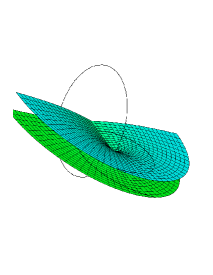
4.1.3 The Dreibein attached to the Dirac point positron
As shown in section 3, evaluated at the worldpoint of the point positron (in the interpretation of [53]) defines a normalized Dreibein “attached” to the point positron at , consisting of the the normalized versions of the orientation vector field given by (18), and its orthogonal complementary vector fields and (constructed in an earlier subsection of section 3), all evaluated at the worldpoint .
Explicitly, expressing in terms of (see section 3.1.3), and evaluating at , we define
| (77) |
and we let denote the actual unit normal vector; similarly we define and as the evaluation of and at the worldpoint , and set and . Then at each , the Dreibein defines a unique element of , say , such that , , and .
4.2 The law of motion for center and orientation of the ring singularity relative to the inertial Dreibein of an infinitely massive point proton at rest
We want to re-interpret the guiding law (75) as supplying also the de Broglie–Bohm–Dirac motion of a spin-1/2 zKN-type ring singularity of mass and charge (as seen in the sheet) which interacts with an infinitely massive point “proton” of charge . Indeed, if in the interpretation of [53] is the initial worldpoint of the point positron, with (say), and is its evolved worldpoint at proper time , then, as explained in subsection 3.2, each quadruplet of these BL coordinates implicitly also describes the actual location of the zKN-type ring singularity of mass and charge relative to the position of that point “positron” — which in the interpretation of this paper becomes an infinitely massive point “proton” with a fixed location — with a Dreibein attached to it which is always a translate of the Dreibein at .
However, since the Dirac equation for a point positron in the static zKN spacetime the Dirac bi-spinor also supplies a frame for the point positron, when re-interpreting the Dirac equation in our sense as an equation for a zKN-type ring singularity moving with respect to a point proton with an inertial frame attached to it, it is clear that there will be a contribution to the velocity of the center of the ring singularity coming from . More precisely, in the interpretation of our current paper, the ring normal now is evolved by the inverse rotation, viz.
| (78) |
This is the law of evolution for the orientation of the ring singularity. The position of the center of the moving ring singularity, , w.r.t. the frame, is simply
| (79) |
Here, is still the proper time along the world line of the “Dirac point positron” from the traditional interpretation; yet since , we can express the evolutions in terms of the reference time of the frame, which coincides with the time of the BL coordinates.
Remark 4.2.
The validity of this re-interpretation of the law of motion is restricted to quasi-static motions relative to the point charge.
4.3 Comments on the de Broglie–Bohm-type laws
4.3.1 Stationary states
Interestingly, in contrast to the non-relativistic de Broglie–Bohm law of electron motion generated from a Schrödinger wave function which yields that for eigenstates the electron sits still (relative to the point “proton”),212121Many physicists have expressed their unease upon learning that de Broglie–Bohm theory predicts that particles don’t move when guided by an eigenstate Schrödinger wave function. However, when compared with Bohr’s famous postulate that the accelerated point charges in the stationary Kepler orbits of his model of the Hydrogen atom move but don’t radiate, thereby denying the predictions of classical electromagnetic theory for such motions even though classical electromagnetism was used in his model to compute the interactions, it seems to us to actually be an asset of the de Broglie–Bohm theory that it resolves Bohr’s dilemma in such a clean way, i.e. in complete agreement with the Maxwell–Lorentz field equations. the de Broglie–Bohm–Dirac law (75) and the orientation law (77) together imply that even for eigenstate bi-spinor wave functions the ring singularity generally does not sit still (relative to the point “proton”). A dynamical ring singularity as source of the Maxwell equations on a zK spacetime would generally be expected to emit electromagnetic radiation; note that in our formulation of the general-relativistic zero- Hydrogen problem in the Born–Oppenheimer approximation radiation is neglected because we are using the quasi-static approximation for the classical electromagnetic fields to compute the interaction energy-momentum vector . So one tentative conclusion is that the inclusion of radiation effects, even if only semi-classically, will possibly destroy most of the energy eigenvalues except perhaps the positive and negative “ground states.” A similar phenomenon is known from so-called “non-relativisitc QED;” in the Hydrogen problem for example, the quantum-mechanical Pauli Hamiltonian for an electron in the Coulomb field of a point proton is additionally coupled to the quantized radiation field, and only the ground state eigenvalue of the Pauli Hamiltonian survives this radiation coupling.
However, at the semi-classical level of electromagnetic coupling that we use here, another possibility is conceivable. Namely, one readily computes that for any solution to Dirac’s equation,
so that is orthogonal to if , which for non-zero and is equivalent to . It is readily checked (see Appendix B) that for eigenstate bi-spinor wave functions , indeed one has . Now for any actual quadruplet the evaluation of can be rotated by an element of to become parallel to computed from this quadruplet (we used this fact already once before, to fix the initial conditions; see above). By the stationarity of the bi-spinor wave function, evaluated with this quadruplet will then remain parallel to computed from this quadruplet for all time. Now, Bohm and Hiley [8] showed in the Pauli limit that the de Broglie–Bohm–Dirac velocity is a vector sum of the de Broglie–Bohm expression one obtains with the Schrödinger equation, plus a gyration that is additionally supplied by the bi-spinor structure of the Dirac equation. Since, as mentioned above, the (what may be called) de Broglie–Bohm–Schrödinger term vanishes for an eigenstate, only the gyrational motion remains. We surmise that this will be so also in the the fully relativistic expression; we have yet to confirm this. But suppose this surmise is correct, then by the axisymmetry of the problem, with this quadruplet interpreted as the actual position of a point “positron” (using again the usual interpretation) we conclude that the point positron moves in a circle parallel to the ring singularity. In the alternate interpretation put forward in the present paper, the point charge is not a point positron but an infinitely massive un-accelerated point “proton,” so from the perspective of that point “proton” the ring singularity now gyrates stationarily about its axis of symmetry, and therefore generates only the static electromagnetic field used to compute the interaction term and no classical electromagnetic radiation fields, in complete agreement with our stationarity assumption.
4.3.2 Quasi-Static Motions
In a non-stationary state the re-interpretation of our Dirac equation as covering the motion of a zKN ring singularity relative to an infinitely massive point proton with Dreibein attached is restricted to the regime of quasi-static motions. This means that the absolute velocities obtained from the gyrational motion need to be much smaller than the speed of light. We now give a rough estimate which shows that for gentle non-stationary perturbations of the Hydrogen ground state we are in the quasi-static regime.
Thus, we recall that the law for the evolution of the orientation vector can be decomposed into a sum of the familiar Larmor formula plus a quantum contribution which contains . We find that for the KN electromagnetic fields a Bohr distance away from the ring singularity the Larmor frequency times the Bohr distance gives a speed of roughly
while the quantum contribution is roughly
So the speed of the ring singularity relative to a point proton with fixed Dreibein, the frame, attached is, in such a situation, roughly one-hundredth the speed of light and thus “quasi-static.”
4.3.3 A Feynman–Stückelberg dilemma avoided
A final remark concerns a dilemma for the de Broglie–Bohm theory when Dirac’s equation is given Dirac’s orginal point electron interpretation or the Stückelberg–Feynman interpretation. Namely the fact that with general initial conditions for both the putative “electronic bi-spinors” and the “positronic bi-spinors” (according to the decomposition of Hilbert space into positive and negative subspaces) enter — and thus also the guiding equation (75) for a single point — is perplexing with these interpretations of Dirac’s equation, while it is completely natural in our interpretation of the Dirac particle as having a bi-particle structure in which electron and anti-electron are merely the “two different sides of the same medal,” realized through a moving zero- Kerr–Newman type ring singularity for which we have formulated a Dirac equation.
5 Outlook
The most important task now would seem to be to numerically evaluate the zKN-Dirac spectrum for the pertinent choice of and see whether the modifications of the Sommerfeld spectrum are physically reasonable. Since the QED corrections like the Lamb shift are spectacular, it would be unwise to expect too much, but it’s certainly an important problem to compute the spectrum quantitatively.
Other important tasks include the discussion of the Hamiltonian in the presence of a zKN-anomalous magnetic moment; as pointed out, we expect that essential self-adjointness holds if the coupling constant is small in magnitude. It is also an interesting question whether more than one self-adjoint extension exists for sufficiently large coupling constant, or none at all. Incidentally, note that our essential self-adjointness result for the Dirac Hamiltonian on the zKN spacetime implies that its naked singularity does no harm.
We have also begun a study of the Dirac Hamiltonian for a zKN ring singularity exposed to a harmonic magnetic field added into the zKN spacetime. We plan to report on this in the future.
Another obviously important question is to tackle the problem of two interacting zKN-like ring singularities, in particular with view toward positronium theory. In that case the Born–Oppenheimer approximation is clearly non-sensical, and one has to face a two-body problem. Here one may hope to benefit from the standard many-body approach detailed in [4].
All these problems should be approachable with the quasi-static approximation invoked here, as long as one is concerned with the discrete spectrum or at most gentle motions.
To go beyond the quasi-static approximation will be a truly challenging task because then one has to contemplate deformations of the ring singularities: stretching, bending, twisting, curling, and who knows what else. It would also require, presumably, solving Einstein’s vacuum equations with such dynamical, topologically ring-like singularities as “boundary condition,” plus the dynamical Maxwell equations on such a spacetime solution with the right asymptotics. In any event, the generalization of Dirac’s equation for this situation should produce the same discrete spectrum as is obtained with the quasi-static approximation.
More speculative, but very tempting and intriguing (to us), are the following thoughts. Namely, since in our interpretation the electron and anti-electron are merely the two different “topo-spin” states of a single more fundamental particle, quite naturally one may wonder whether in the many-body theory there is an analog of a ferro-magnetic phase transition — this would require a statistical mechanical analysis in the limit of infinitely many zKN ring singularities. This phase transition would of course not be the magnetization phase transition, but in the topo-spin space, and amount to the emergence of a broken symmetry phase in which only electrons (or only positrons) feature in one sheet of physical space. This would offer a completely novel explanation of the apparently broken particle/anti-particle symmetry in our world!
All of the above invokes the zero-gravity limit. Ultimately one wants to switch gravity back on again, not because one should expect significant corrections to the atomic spectra, but for conceptual reasons. However, as we have recalled, for the maximal-analytically extended Kerr–Newman solution suffers from causal pathologies and strong curvature singularities which — quite possibly — are unphysical. Upon closer inspection one can trace the origin of these pathologies to the linear Maxwell–Maxwell222222By speaking of the Maxwell–Maxwell system, the first “Maxwell” stands for the so-called pre-metric Maxwell equations, while the second “Maxwell” stands for the “law of the electromagnetic vacuum” (in condensed matter physics called the “constitutive relations”) connecting the four electromagnetic three-component fields of the pre-metric equations. Thus, in Minkowski spacetime, in a space time splitting of the Faraday tensor into and of the Maxwell tensor into , choosing Maxwell’s “law of the pure ether” and yields the Maxwell–Maxwell equations (and the general relativistic model becomes the Einstein–Maxwell–Maxwell equations). A physically potentially important nonlinear law of the electromagnetic vacuum is due to Born and Infeld [13], in which case we shall speak of Maxwell–Born–Infeld, respectively Einstein–Maxwell–Born–Infeld equations; see [52] for a recent discussion of their physical significance. As long as we work with the default choice of Maxwell’s “law of the pure ether” we simply drop the second “Maxwell,” but retain it in discussions in which it is important to distinguish these from e.g. the Einstein–Maxwell–Born–Infeld equations. equations which for point and ring sources produce solutions with non-integrable field-energy densities; when coupled to the spacetime structure through the Einstein–Maxwell–Maxwell equations, the consequences are devastating. Thus, before any physically meaningful deformation of the zero- results to can be attempted, first one has to redo the zero- calculations with the linear Maxwell–Maxwell equations replaced by better-behaved equations that yield integrable energy densities for point and ring charges, for instance the nonlinear Maxwell–Born–Infeld equations, then deform into the full system of Einstein–Maxwell–Born–Infeld equations. So far this has only been accomplished for a single point charge [76] in a topologically simple spacetime, but we don’t see any reason for why this should not be possible for spacetimes with Zipoy topology and their ring singularities. Of course, progress may come slowly.
Acknowledgement: This work did not grow in a vacuum but in the stimulating “fundamental physics research” atmosphere created by our colleages at Rutgers, in particular Joel Lebowitz, Shelly Goldstein, Rodi Tumulka, Avy Soffer, and Eric Carlen. We thank all of them. We thank Shelly Goldstein also for pointing out Dankel’s work, and Rodi Tumulka for clarifying discussions about the de Broglie–Bohm laws of evolution. Thanks go also to Friedrich Hehl for his many encouraging comments. We thank Barry Simon for his remarks on perturbation theory. We thank Ted Newman for his interesting comments, and for his permission to quote from one of his communications he sent us. Lastly, we thank the referees for their thoughtful comments.
Appendix
A: From and to oblate spheroidal coordinates
Let be a unit vector, representing the orientation of the ring, i.e. the ring lies in a plane with unit normal and is positively oriented with respect to . Next we introduce oblate spheroidal coordinates centered at in order to generate a copy of zKN with the ring singularity of radius centered at and axis of symmetry parallel to the axis. These coordinates are defined as follows: let , and define and as follows
| (80) | |||||
| (81) |
The oblate spheroidal coordinates are closely related to cylindrical coordinates: Let
| (82) | |||||
| (83) | |||||
| (84) |
( is the Heaviside function) be cylindrical coordinates centered at and with symmetry axis parallel to . We then have the following change of coordinate formula
In particular, the set of points where is a 2-disc in ,
and the ring is the boundary of this disc. The level sets of are oblate spheroids, and those of are one-sheeted hyperboloids. As was mentioned before, the coordinate can be extended to take on negative values, and the physical space is likewise extended to become a double-sheeted branched Riemann space [33]. The set of points gives us a copy of a spatial slice of the maximal extension of zKN, which we denote by .
Consider now a point particle with location . The locus of possible ring centers with ring normal such that the point particle sits somewhere on that ring, is itself a ring of the same radius, this one around the point particle. Suppose then that we introduce cylindrical coordinates centered at with symmetry axis , in the same manner as in the above. Let denote the location of the geometric center of the ring in the primed coordinates based at the point particle. One easily checks that
Let be oblate spheroidal coordinates based at . Then likewise we have
It now follows that the interaction potential can be equally well expressed in the primed coordinates:
Indeed the only difference in the expression for the interaction potential would be that the sign of is flipped. However, since the geometrical center of the ring singularity has no ontological significance, we invoke only as auxiliary variable and therefore also not use its oblate spheroidal coordinates based at , but instead work with the original oblate spheroidal coordinates .
B: Separation of variables for the Dirac Equation on a zKN spacetime
When the Dirac equation (61) for the bi-spinor allows a clear separation also for the remaining and derivatives (commonly referred to in the literature as “radial” and “angular” derivatives, even though is not a radius and is not an angle, except at infinity). Thus, when the Dirac equation (61) becomes
| (85) |
where
| (90) | |||||
| (95) |
where and have been given in (44). Once a solution to (85) is found, the bi-spinor solves the original Dirac equation (21).
Following Chandrasekhar we make the Ansatz that a solution of (85) is of the form
| (96) |
with being complex-valued functions of alone, and real-valued functions of alone. Let
| (97) |
Plugging the Chandrasekhar Ansatz (96) into (85) one easily finds that there must be such that
| (98) |
| (99) |
where
| (102) | |||||
| (105) |
The operators and are now ordinary differential operators in and respectively, with coefficients that depend on the unknown , and parameters , , and :
| (106) | |||||
| (107) |
The angular operator in (99) is easily seen to be essentially self-adjoint on and in fact is self-adjoint on its domain inside (e.g. [74, 3]) with purely point spectrum , . Thus in particular . It then follows that the radial operator is also essentially self-adjoint on and in fact self-adjoint on its domain inside
Suppose is a non-trivial solution to , with . Then
Multiply the first equation by and the second equation by , add them and take the real part, to obtain
| (108) |
Thus the difference of the moduli squared of and is constant, hence zero since they need to be integrable at infinity. I.e.,
| (109) |
Let for . Multiply the first equation by , multiply the complex conjugate of the second equation by , and add them to obtain
| (110) |
Thus the ratio , and hence the sum of the arguments must be a constant, say . Thus . Since multiplication by a constant phase factor is a gauge transformation for Dirac bi-spinors, we can replace with without changing anything. The spinor thus obtained has the same form as (96), now with . Thus without loss of generality we can assume and .
This motivates us to set
| (111) |
for real functions and . Consider the unitary matrix
| (112) |
A change of basis using brings the radial system (98) into the following standard (Hamiltonian) form
| (113) |
where
| (114) |
(cf. [81], eq (7.105)) with
| (115) |
Consider now the equations (113) and (99) for unknowns and . Let us define new unknowns and via the Prüfer transform [68]
| (116) |
Thus
| (117) |
As a result, and . Hence can be re-expressed in terms of the Prüfer variables, thus
| (118) |
and we obtain the following equations for the new unknowns
| (119) | |||||
| (120) |
Similarly,
| (121) | |||||
| (122) |
In [53] we show that the above equations, under suitable assumptions on the parameters, have solutions that give rise to an eigenstate .
We conclude by noting that, via a slight change in notation, (118) can be brought to the generalized Cayley-Klein form (17), namely, setting
one obtains
| (123) |
In particular, for bi-spinors of this type, , so that and thus, per discussion in 4.3, the resulting motion of the ring is a stationary circulation.
C: Other proposals to link Dirac’s equation and the Kerr–Newman spacetime.
To be sure, we are not the first ones to suspect a connection between the Kerr–Newman (KN) spacetime and the Dirac electron,232323Judged by his early speculations [31], Einstein could have been tempted, too, had he been around in the 60s. recall footnote 10. Speculations in this direction seem to have appeared first in Carter’s paper [19], where he observed that the Kerr–Newmann solution features a -factor of 2, just like Dirac’s wave equation for the electron. Subsequently this idea was picked up by others, see in particular [67, 59, 2, 17], and related papers mentioned below. However, all these earlier proposals have run into grave difficulties. To some measure these are caused by the physically questionable character of the KN solution with , unveiled by Carter [19] (see also [42, 65]), while the proposals in [67, 59] suffer from artificial infinities introduced by truncating the zKN manifold to obtain a topologically simple spacetime.
As to its questionable character, the maximal-analytical extension of the axisymmetric and stationary “outer” KN spacetime with [19] has a very strong curvature singularity on a timelike cylindrical surface whose cross-section with constant- hypersurfaces is a circle; here, is a coordinate pertinent to the asymptotically (at spacelike ) timelike Killing field that encodes the stationary character of the “outer regions” of the KN spacetime. This circle is commonly referred to as the “ring” singularity. The region near the ring is especially pathological since it includes closed timelike loops.242424The timelike ring singularity of the KN manifold is itself the limit of closed timelike loops. Anybody unfortunate enough to be trapped in this region is doomed to repeat the same mistakes over and over again. In the black-hole sector of the parameter space of the KN family of spacetimes this acausal region is “hidden” behind an event horizon, but the electron parameter values are not in this black-hole sector, the ring singularity is then “naked,” and the closed timelike loops turn the entire manifold into a causally vicious set.
As pointed out earlier, it was also discovered in [19] that the ring singularity is associated with the topologically non-trivial feature that the maximal-analytical extension of the KN spacetime consists of two asymptotically flat ends which are “doubly linked through the ring.” Carter showed that this Zipoy topology survives the vanishing-charge limit of the KN manifold, which yields the maximal-analytic extension [14] of Kerr’s solution [50] to Einstein’s vacuum equations, cf. [41]. He furthermore showed that this topology survives the vanishing-mass limit of the Kerr manifold, which yields an otherwise flat vacuum spacetime, which is also the vanishing-mass limit of a static spacetime family discovered and completely described a few years earlier by Zipoy [86].
We emphasize that its nontrivial topology is not necessarily a physically questionable feature of the maximal-analytically extended Kerr–Newman solution to the Einstein–Maxwell equations, in the sense that it is not an arbitrary mathematical construct, does not seem to lead to paradoxical conclusions, and no empirical data seem to rule it out yet. Yet it is frequently perceived as a physically questionable feature. In particular, some general relativists seem to abhor such topologically non-trivial spacetimes,252525Unfortunately this attitude can be encountered even nowadays, despite the ubiquity of topologically non-trivial Calabi–Yau manifolds in string theory. as exemplified by the following quote from [10]: “[Zipoy] endowed [his spacetimes] with rather terrifying topological properties.” Guided by similar sentiments, and following [10] in their treatment of the Zipoy spacetimes, Israel [46] engineered a single-leafed electromagnetic spacetime, obtained from half of the maximal-analytically extended KN manifold by identifying the limit points of sequences which approach the disc spanned by the ring from above with those approaching it from below, in one and the same leaf. However, this “short-circuiting” procedure produces a spacetime with an ultra-singular disc source:262626Incidentally, for astrophysical interpretations of the Kerr–Newman spacetime (other than a black hole) another cut-and-short-circuiting procedure has been proposed in attempts to find a singular disc source for the spacetime and its electromagnetic fields; see [57, 36], and also [5] for the Kerr spacetime. This results in an infinitely extended, infinitely thin disc source which is not as physically bizarre as the “disc source” spanned by the KN ring singularity. the disc’s interior carries an infinite total charge and current, and with the wrong sign on top of that, which have to be “partly compensated” by an infinite opposite charge and current on its rim to leave a finite net amount of charge and current as diagnosed by the asymptotic flux integrals; see [46], and also [67]. Furthermore, the disc holds a negative infinite amount of mass in its interior, to be “compensated partly” by a positive infinite amount of mass on its rim in order to produce the ADM mass, and it rotates at superluminal speeds [46]. The mathematically artificial construction of a topologically simple spacetime with a “disc source” of such physically bizarre proportions is, in our opinion, too high a price to pay to satisfy — what to us seems to have been — just a prejudice against topologically non-trivial spacetimes,272727It is quite an irony of sorts that 35 years earlier Einstein, prejudiced at the time against singularities, together with Rosen [32] envisaged a topologically non-trivial linkage (the so-called Einstein–Rosen bridge) of two copies of an outer region of the Schwarzschild manifold in order to avoid its singularities. As known nowadays, “the Einstein–Rosen bridge cannot be crossed,” yet it is part of the maximal-analytical extension of the outer region of the Schwarzschild manifold [56, 75], which — ironically, too — is topologically simple, yet singular, having the past and future, spacelike curvature singularities which Einstein hoped to avoid. expressed in [10, 46]. Lastly, there still is a region of closed timelike loops in Israel’s single-leafed spacetime.282828To the extent that it has been addressed at all in the pertinent literature, it has only been pointed out that in the zero-charge limit the acausal region is excised by the cutting and short-circuiting process [46], yet in a footnote Israel notes that in the charged situation some acausal region remains after the cutting and short-circuiting.
By contrast, Arcos and Pereira [2] embrace the topologically non-trivial character of the maximal analytically extended Kerr–Newman spacetime. Yet, also these authors cut and re-glue the KN manifold, though in a different way. Namely, in [2] it is argued that the acausal region has to be “cut out” and its boundary “re-glued.” Thereby the ring singularity is removed as well, leading to a manifold in the spirit of John Wheeler’s “charge without charge” [84]. Unfortunately, as noted in [2], their manifold has the non-orientable topology of a Klein bottle. Furthermore, the authors of [2] only claim the continuity of the metric but do not investigate the higher regularity of the metric and electromagnetic fields across the re-glued cut, and in fact their gluing process may well have introduced some artificial singularities.
Also in contrast to [46, 67, 59], the authors of [2] actually try to establish a mathematical connection between the electromagnetic Kerr–Newman manifold and the Dirac equation for the electron beyond the fact that both feature a -factor of 2. Interestingly enough, they propose to identify their cut-and-re-glued Kerr–Newman spacetime itself with a bi-spinor solution of Dirac’s equation, by mapping the metric components of their manifold into the components of a Dirac bi-spinor which satisfies a Dirac equation for the free electron; a similar proposal was made in [17]. However, such an identification is conceptually unstable under perturbations: first, a Dirac bi-spinor does not have enough degrees of freedom to map into a solution of the Einstein–Maxwell equations in a generic neighborhood of the KN solution; and second, a Dirac bi-spinor satisfying a Dirac equation for a non-free electron will hardly produce a Lorentzian metric (whether using the mapping of [2] or of [17]) that solves the Einstein–Maxwell equations. Thus, the possibility of such an identification for the KN manifold, should it pan out rigorously, would rather seem to be a mathematical curiosity without deeper physical implications.
By considering the zero- limit of the maximal-analytically extended KN spacetime we are avoiding all the acausal and other pathological features of that spacetime which have prompted the ad-hoc surgical procedures in the studies of [2] and [17] that involve the removal of the ring singularity. In particular, we are able to compute the electromagnetic interaction between the zKN ring singularity and a point charge at rest elsewhere in the zKN spacetime which provides the interaction term in Dirac’s equation — something that is manifestly impossible in the approaches of [2] and [17].
Also others, in particular Lynden-Bell [59] and co-workers [35], have contemplated the zero- limit of the Kerr–Newman spacetime as a better candidate to provide a link between general relativity and the electron. However, these authors do not consider the maximal-analytical extension but, following Israel’s lead [46], introduce an artificial branch cut at the disc spanned by the ring. As pointed out in [46], it is possible to interpret the KN electromagnetic fields on Minkowski spacetime, which is the zero- limit of Israel’s single-leafed short-circuited truncation of the maximal-analytically extended KN spacetime. Kaiser [48] finds that interpreted in this way the superluminal speeds are absent, and the rim of the disc rotates exactly at the speed of light; still the interior of the disc carries an infinite total charge and current which are “partly compensated” by an infinite opposite charge and current on the rim of the disc, leaving a finite net amount of charge and current as diagnosed by the usual asymptotic formulas of classical electromagnetism. Undeterred by such warning signs, it has been speculated in [59] “that something similar may occur in the quantum electrodynamic charge distribution surrounding the point electron.”
Since nature has her own ways, perhaps she does associate electrons with such ultra-singular discs. However, we have serious doubts that there is any fundamental physical truth in this notion. In particular, from a mathematical point of view the “disc singularity of the Kerr–Newman manifold” is an artificial construct, akin to a branch cut, obtained by arbitrarily292929There are uncountably many other ways to cut and then short-circuit one of the so obtained leaves, and each of these artificially-so-created singularities could be claimed to be “the source of the Kerr–Newman fields.” One may want to argue that the disc is special because the maximal-analytically extended Kerr–Newman manifold has a reflection symmetry which leaves the disc spanned by the ring singularity invariant, and this is inherited by the “Kerr–Newman manifold with disc singularity;” but that symmetry remains intact also if one cuts along a sphere with the ring singularity as equator, then identifies points in the two hemispheres by reflection. choosing the disc spanned by the ring singularity for cutting the maximal-analytically extended Kerr–Newman manifold, then discarding half of it, and short-circuiting the remaining part at the cut.
Besides introducing mathematically artificial pathologies, in Israel’s one-leaved truncation of the maximal-analytically extended zero- Kerr–Newman spacetime the crucial electromagnetic bi-particle structure of the zKN ring singularity is lost, while for us it is the main feature needed to coherently interpret the spectral properties of “Dirac’s wave equation for the electron.”
Furthermore, as far as we can tell, all previous proposals to link the KN manifold with “Dirac’s equation for the electron” invariably invoke Carter’s observation that the gyromagnetic ratio of this electromagnetic spacetime (i.e. by definition the ratio of its total magnetic moment to its total angular momentum) is equal to q/m, which coincides with the value predicted for the electron by the one-body Dirac equation. Yet note that in the zero- limit the KN spacetime becomes static so that it becomes nonsensical to speak of its gyro-magnetic ratio, indicating that the -factor may be a false lead. Of course, one may still assign an angular momentum to the ring singularity, but how to do it unambiguously is not clear.
Lastly, to the extend that an estimate of the radius of the KN singularity has been attempted in earlier proposals that try to link the KN manifold with “Dirac’s equation for the electron,” the suggestive identification of the Kerr–Newman magnetic moment with the Bohr magneton is made, which leads to . In contrast to such estimates, our spectral analysis shows that the Bohr magneton is supplied already by the structure of Dirac’s equation for a point particle featuring an electric monopole but no magnetic dipole, so that the magnetic moment carried by the zKN ring singularity is to be identified with the electron’s anomalous magnetic moment, yielding a significantly smaller ring radius than in all the other studies.
References
- [1] P. Appell. Quelques remarques sur la théorie des potentiels multiforms. Math. Ann., 30:155–156, 1887.
- [2] H. I. Arcos and J. G. Pereira. Kerr-Newman solution as a Dirac particle. Gen. Rel. Grav., 36:2441–2464, 2004.
- [3] D. Batic, H. Schmid, and M. Winklmeier. On the eigenvalues of the Chandrasekhar-Page angular equation. J. Math. Phys., 46(1):012504, 35, 2005.
- [4] H. A. Bethe and E. E. Salpeter. Quantum Mechanics of One- and Two-Electron Atoms. Plenum Press, 1977.
- [5] J. Bičák and T. Ledvinka. Relativistic disks as sources of the Kerr metric. Phys. Rev. Lett., 71:1669–1672, 1993.
- [6] D. Bohm. A suggested interpretation of the quantum theory in terms of “hidden” variables. part I. Phys. Rev., 85:166–179, 1952.
- [7] D. Bohm. A suggested interpretation of the quantum theory in terms of “hidden” variables. part II. Phys. Rev., 85:180–193, 1952.
- [8] D. Bohm and B. Hiley. The undivided universe. Routledge, London & New York, 1993.
- [9] D. Bohm, R. Schiller, and J. Tiomno. A causal interpretation of the Pauli equation (A). Nuovo Cim. Suppl., 1:48–66, 1955.
- [10] W. B. Bonnor and A. Sackfield. The interpretation of some spheroidal metrics. Commun. Math. Phys., 8:338–344, 1968.
- [11] M. Born. Quantenmechanik der Stossvorgänge. Z. Phys., 38:803–827, 1926.
- [12] M. Born. Zur Quantenmechanik der Stossvorgänge. Z. Phys., 37:863–867, 1926.
- [13] M. Born and L. Infeld. Foundation of the new field theory. Proc. Roy. Soc. London, A 144:425–451, 1934.
- [14] R. H. Boyer and R. W. Lindquist. Maximal analytic extension of the Kerr metric. J. Math. Phys., 8(2):265–281, 1967.
- [15] D. R. Brill and J. M. Cohen. Cartan frames and the general relativistic Dirac equation. J. Math. Phys., 7(2):238–243, 1966.
- [16] G. E. Brown and D. G. Ravenhall. On the interaction of two electrons. Proc. Roy. Soc. London, A, 208:552–559, 1951.
- [17] A. Burinskii. The Dirac–Kerr-Newman electron. Grav. Cosmol., 14:109–122, 2008.
- [18] E. Cartan. Theory of Spinors. MIT, Cambridge MA, 1966; repr. Dover, 1983.
- [19] B. Carter. Global structure of the Kerr family of gravitational fields. Phys. Rev., 174:1559–1571, 1968.
- [20] B. Carter and R. G. McLenaghan. Generalized master equations for wave equation separation in a Kerr or Kerr-Newman black hole background. In R. Ruffini, editor, Proceedings of the second Marcel Grossmann meeting on general relativity, pages 575–585. North-Holland Publishing Company, 1982.
- [21] S. Chandrasekhar. Errata: “The solution of Dirac’s equation in Kerr geometry”. Proc. Roy. Soc. London Ser. A, 350(1663):565, 1976.
- [22] S. Chandrasekhar. The solution of Dirac’s equation in Kerr geometry. Proc. Roy. Soc. London Ser. A, 349(1659):571–575, 1976.
- [23] T. G. Dankel. , Jr. Mechanics on manifolds and the incorporation of spin into Nelson’s Stochastic mechanics. Arch. Rat. Mech. Anal., 37:192–221, 1970.
- [24] C. G. Darwin. The wave equation of the electron. Proc. Roy. Soc. London, A118:654–680, 1928.
- [25] L. C. Davis and J. R. Reitz. Solution to potential problems near a conducting semi-infinite sheet or conducting disk. Amer. J. Phys., 39(10):1255–1265, 1971.
- [26] L. V. de Broglie. La nouvelle dynamique des quanta. In J. Bordet, editor, Cinquième Conseil de Physique Solvay, Bruxelles, 1927. Gauthier-Villars et Cie., Paris, 1928. English translation: “The new dynamics of quanta”, p.374-406 in: Bacciagaluppi, G., and Valentini, A., Quantum Theory at the Crossroads, Cambridge Univ. Press, 2013.
- [27] D. Dürr, S. Goldstein, K. Münch-Berndl, and N. Zanghì. Hypersurface Bohm–Dirac models. Phys. Rev., A 60:2729–2736, 1999.
- [28] D. Dürr, S. Goldstein, and N. Zanghì. Quantum Physics Without Quantum Philosophy. Springer, 2013.
- [29] D. Dürr and S. Teufel. Bohmian Mechanics: The Physics and Mathematics of Quantum Theory. Springer, 2012.
- [30] A. B. Efimov and V. N. Vorob’ev. A mixed boundary-value problem for the Laplace equation. Journal of engineering physics, 26(5):664–666, 1974.
- [31] A. Einstein. Spielen Gravitationsfelder im Aufbau der materiellen Elementarteilchen eine wesentliche Rolle? Sitzungsber. der Preuss. Akad. der Wiss., Berlin, pages 349–356, 1919.
- [32] A. Einstein and N. Rosen. The particle problem in the general theory of relativity. Phys. Rev., 48:73–77, 1935.
- [33] G. C. Evans. Lectures on Multiple-Valued Harmonic Functions in Space. Univ. of California Press, Berkeley and Los Angeles, 1951.
- [34] R. P. Feynman. Theory of positrons. Phys. Rev., 76:749–759, 1949.
- [35] J. R. Gair and D. Lynden-Bell. Electromagnetic fields of separable spacetimes. Class. Quant. Grav., 24(6):1557, 2007.
- [36] G. García-Reyes and G. A. Gonzáles. Rotating and counterrotating relativistic thin disks as sources of stationary electrovacuum spacetimes. Brazil. J. Phys., 37:1094–1105, 2007.
- [37] I. M. Glazman. Direct methods of qualitative spectral analysis of singular differential operators. Israel Prog. Sci. Transl., Jerusalem, 1965.
- [38] H. Goldstein. Classical Mechanics. Addison-Wesley, Cambridge, MA, 1980.
- [39] W. Gordon. Die Energieniveaus des Wasserstoffatoms nach der Diracschen Quantentheorie des Elektrons. Z. Phys., 48:11–14, 1928.
- [40] W. Greiner, B. Müller, and J. Rafelski. Quantum electrodynamics of strong fields. Springer, 1985.
- [41] S. Hawking and G. Ellis. The Large Scale Structure of Space-Time. Cambridge Univ. Press, Cambridge, 1973.
- [42] C. Heinicke and F. W. Hehl. Schwarzschild and Kerr solutions of Einstein’s field equation: An introduction. Int. J. Mod. Phys. D, 2015.
- [43] E. W. Hobson. On Green’s function for a circular disk, with applications to electrostatic problems. Trans. Cambridge Phil. Soc, 18:277–291, 1900.
- [44] P. R. Holland. Causal interpretation of a system of two spin-1/2 particles. Physics Reports (Review Section of Physics Letters), 169(5):293–327, 1988.
- [45] P. R. Holland. The Quantum Theory of Motion: An Account of the de Broglie–Bohm causal Interpretation of Quantum Mechanics. Cambridge Univ. Press, 1993.
- [46] W. Israel. Source of the Kerr metric. Phys. Rev. D (3), 2:641–646, 1970.
- [47] J. D. Jackson. Classical Electrodynamics. Wiley, New York, 2nd edition, 1975.
- [48] G. Kaiser. Distributional sources for Newman’s holomorphic Coulomb field. J. Phys. A, 37(36):8735, 2004.
- [49] S. Keppeler. Spinning Particles - Semiclassics and Spectral Statistics. Springer, 2003.
- [50] R. P. Kerr. Gravitational field of a spinning mass as an example of algebraically special metrics. Phys. Rev. Lett., 11:237–238, 1963.
- [51] M. K.-H. Kiessling. Misleading signposts along the de Broglie-Bohm road to quantum mechanics. Found. Phys., 40:418–429, 2010.
- [52] M. K.-H. Kiessling. On the motion of point defects in relativistic fields. In F. Finster, O. Müller, M. Nardmann, J. Tolksdorf, and E. Zeidler, editors, Quantum Field Theory and Gravity. Conceptual and mathematical advances in the search for a unified framework, (Regensburg, Sept. 28 – Oct. 1, 2010), pages 299–335. Birkhäuser, Basel, 2012.
- [53] M. K.-H. Kiessling and A. S. Tahvildar-Zadeh. The Dirac point electron in zero-gravity Kerr-Newman spacetime. J. Math. Phys., 56:042303 (43), 2015.
- [54] M. K.-H. Kiessling and A. S. Tahvildar-Zadeh. Dirac’s point electron in the zero-gravity Kerr–Newman world. In F. Finster, J. Tolksdorf, and E. Zeidler, editors, Quantum Mathematical Physics (Regensburg, Sept. 29–Oct. 2, 2014), page 26pages. Birkhäuser, Basel, 2016.
- [55] W. Kinnersley. Type D vacuum metrics. J. Math. Phys., 10:1195, 1969.
- [56] M. D. Kruskal. Maximal extension of Schwarzschild metric. Phys. Rev., 119:1743–1745, 1960.
- [57] T. Ledvinka, M. Žofka, and J. Bičák. Relativistic disks as sources of Kerr–Newman fields. In R. Ruffini, editor, Proceedings of the eighth Marcel Grossmann meeting on general relativity, Jerusalem (1997). World Scientific, Singapore, 1998.
- [58] E. H. Lieb and R. Seiringer. The Stability of Matter in Quantum Mechanics. Cambridge Univ. Press, Cambdridge, UK, 2010.
- [59] D. Lynden-Bell. Electromagnetic magic: The relativistically rotating disk. Phys. Rev. D, 70:105017, Nov 2004.
- [60] A. Messiah. Quantum Mechanics, volume II. North Holland Publishing Company, 1965.
- [61] C. Neumann. Über die peripolaren Koordinaten. Abh. math.-phys. Classe königl. sächs. Ges. Wiss., 12:365–398, 1880.
- [62] S. F. Neustadter. Multiple valued harmonic functions with circle as branch curve, volume 1. University of California Press, 1951.
- [63] E. T. Newman. Classical, geometric origin of magnetic moments, spin-angular momentum, and the Dirac gyromagnetic ratio. Phys. Rev. D, 65:104005, Apr 2002.
- [64] E. T. Newman, E. Couch, K. Chinnapared, A. Exton, A. Prakash, and R. Torrence. Metric of a rotating, charged mass. J. Math. Phys., 6(6):918–919, 1965.
- [65] B. O’Neill. The Geometry of Kerr black holes. L.K. Peters, Wellesley, 1995.
- [66] D. Page. Dirac equation around a charged, rotating black hole. Phys. Rev. D, 14:1509–1510, 1976.
- [67] C. L. Pekeris and K. Frankowski. The electromagnetic field of a Kerr-Newman source. Phys. Rev. A (3), 36(11):5118–5124, 1987.
- [68] H. Prüfer. Neue Herleitung der Sturm-Liouvilleschen Reihenentwicklung stetiger Funktionen. Math. Ann., 95(1):499–518, 1926.
- [69] R. Schiller. Quasi-classical theory of a relativistic spinning electron. Phys. Rev., 128(3):1402, 1962.
- [70] S. Schweber. QED and the men who made it: Dyson, Feynman, Schwinger, and Tomonaga. Princeton Univ. Press, Princeton, 1994.
- [71] A. Sommerfeld. Über verzweigte Potentiale im Raum. Proc. London Math. Soc., s1-28(1):395–429, 1896.
- [72] N. Straumann. General Relativity and Relativistic Astrophysics. Springer-Verlag, Berlin, 1984.
- [73] E. C. G. Stückelberg. La mécanique du point matériel en théorie de relativité et en théorie des quanta. Helv. Phys. Acta, 15:23–37, 1942.
- [74] K. G. Suffern, E. D. Fackerell, and C. M. Cosgrove. Eigenvalues of the Chandrasekhar–-Page angular functions. J. Math. Phys., 24(5):1350–1358, 1983.
- [75] G. Szekeres. On the singularities of a Riemannian manifold. Pub. Math. Debrecen, 7:285ff, 1960. Reprinted in Gen. Rel. Grav. vol. 34, issue 11, pp. 2001–2016 (2002).
- [76] A. S. Tahvildar-Zadeh. On the static spacetime of a single point charge. Rev. Math. Phys., 23(3):309–346, 2011.
- [77] A. S. Tahvildar-Zadeh. On a zero-gravity limit of the Kerr–Newman spacetimes and their electromagnetic fields. J. Math. Phys., 56:042501 (19), 2015.
- [78] D. V. Tausk and R. Tumulka. Can we make a Bohmian electron reach the speed of light, at least at one instant? J. Math. Phys., 51:122306 (19), 2010.
- [79] S. A. Teukolsky. Rotating black holes: Separable wave equations for gravitational and electromagnetic perturbations. Phys. Rev. Lett., 29(16):1114, 1972.
- [80] B. Thaller. Potential scattering of Dirac particles. J. Phys. A: Math. Gen., 14:3067–3083, 1981.
- [81] B. Thaller. The Dirac equation. Springer-Verlag, Berlin, 1992.
- [82] N. Toop. The thermal radiation of electrons from a charged spinning black hole in a cosmological background. preprint DAMTP, Cambridge, 1976.
- [83] J. Weidmann. Absolut stetiges Spektrum bei Sturm-Liouville-Operatoren und Dirac-Systemen. Math. Z., 180(2):423–427, 1982.
- [84] J. A. Wheeler. Geometrodynamics. Academic Press, New York, 1962.
- [85] M. Winklmeier and O. Yamada. A spectral approach to the Dirac equation in the non-extreme Kerr-Newmann metric. J. Phys. A, 42(29):295204, 15, 2009.
- [86] D. M. Zipoy. Topology of some spheroidal metrics. J. Math. Phys., 7(6):1137–1143, 1966.