On Finding Minimal Infrequent Elements in Multi-dimensional Data Defined over Partially Ordered Sets

Abstract

We consider databases in which each attribute takes values from a partially ordered set (poset). This allows one to model a number of interesting scenarios arising in different applications, including quantitative databases, taxonomies, and databases in which each attribute is an interval representing the duration of a certain event occurring over time. A natural problem that arises in such circumstances is the following: given a database $\mathcal{D}$ and a threshold value $t$, find all collections of ”generalizations” of attributes which are ”supported” by less than $t$ transactions from $\mathcal{D}$. We call such collections infrequent elements. Due to monotonicity, we can reduce the output size by considering only minimal infrequent elements. We study the complexity of finding all minimal infrequent elements for some interesting classes of posets. We show how this problem can be applied to mining association rules in different types of databases, and to finding ”sparse regions” or ”holes” in quantitative data or in databases recording the time intervals during which a re-occurring event appears over time. Our main focus will be on these applications rather than on the correctness or analysis of the given algorithms.

Keywords: Association rules, categorical attributes, enumeration algorithms, frequent/infrequent elements, intervals, lattices, maximal empty boxes, partially ordered sets, quantitative data, rare associations, taxonomies.

1 Introduction

The problem of mining association rules from large databases has emerged as an important area of research since their introduction in [AIS93]. Typically, the different data attributes exhibit certain correlations between them, which can be summarized in terms of certain rules, provided that enough transactions or records in the database agree with these rules. For a few examples, in a database storing sets of items purchased by different customers in a supermarket, it may be interesting to observe a rule of the from ”most customers that purchase bread and butter tend also to purchase orange juice”; in a database storing personal data about individuals, it may be interesting to observe that ”most individuals who are married and with age in the range 28-34 have at least 2 cars”; and in a database storing data about the time periods a given service is used by different customers, an interesting observation may take the form: ” customers who make full use of the service between 2:00-3:00 on Friday tend also to use the service between 2:00-3:00 on Saturday”. Such information could be useful, for example, for placing items next to each other on supermarket shelves or providing better services for anticipated customers.

Most of the work on finding association rules divides the task into two basic steps: the first one is to identify those collections of items or attribute values that appear together frequently in the database, the so-called frequent itemsets; the second step is to generate association rules from these. While the first step has received considerable attention in the literature, with many algorithms proposed, the second step seems to be somehow overlooked. In this chapter, we will have a more careful look at this latter step, and show in fact that a lot of redundancy can be eliminated from the generated rules by solving the somewhat complementary problem of finding infrequent sets, i.e., those collection of items that rarely appear together in any transaction. This gives one important motivation for studying the problem of finding infrequent collections of values that can be assumed by the attributes of the given database. But apart from that, finding such collections is a problem of independent interest, since each infrequent collection of attribute values indicates rare associations between these values. For instance, in the database of personal data above one can observe a rule like ”no individuals with age between 26 and 38 have a single car”, and in the database recording service usage, one may observe that “Fewer than 40% of the customers occupy the service on Friday between 2:00-3:00 and on Saturday between 2:00-4:00”. Another application will be given in Section 4.2, in which the objective is to discover the so-called rare association rules, which are informally rules that result from data appearing rarely in the database.

Rather than using binarization, as is common in the literature (see e.g. [SA95, SA96]), to represent the different ranges of each attribute by binary values, we shall consider more generally databases in which each attribute assumes values belonging to a partially ordered set (poset). This general framework will allow us to model a number of different scenarios in data mining applications, including the mining of association rules for databases with quantitative, categorical and hierarchical attributes, and the discovery of missing associations or “holes” in data (see [AMS+96, LKH97, BLQ98]). One important feature of this framework is that it allows us to find generalized associations, which are obtained by generalizing some attribute values, for which otherwise there exist no enough support from the database transactions. As an example on the supermarket data above, it may be the case that most customers who purchase milk products tend also to purchase bread, but in the database only ”cheese” and ”butter” appear as items. In this case generalizing both these items to ”milk products” allows us to discover the above rule.

We begin our exposition in the next section with recalling some definitions and terminology related to partially ordered sets and give some examples of databases defined over products of posets. In Section 3, we define the main object of interest in this chapter, namely minimal infrequent elements in products of posets, describe the associated enumeration problem, and discuss how to measure its complexity. Section 4 gives some applications of such enumeration problems to finding association rules in different types of databases and to finding sparse regions on quantitative data. In Section 5, we discuss briefly the complexity of finding infrequent/minimal infrequent elements, with more details provided in the appendix for the interested reader. We conclude in Section 6 with pointers to implementation issues and some open problems.

2 Databases defined on products of partially ordered sets

Recall that a partially ordered set (poset) is defined by a pair $(\mathcal{P},\preceq)$, where $\mathcal{P}$ is a finite set and $\preceq$ is a binary relation satisfying the following three properties:

1. reflexivity: $a\preceq a$ for all $a\in\mathcal{P}$;

2. anti-symmetry: if $a\preceq b$ and $b\preceq a$ then $a=b$;

3. transitivity: if $a\preceq b$ and $b\preceq c$ then $a\preceq c$.

Let $\mathcal{P}$ be (the ground set of) a poset. Two elements $x,y$ in $\mathcal{P}$ are said to be comparable if either $x\preceq y$ or $y\preceq x$ and otherwise are said to be incomparable. A chain (anti-chain) of $\mathcal{P}$ is subset of pairwise comparable (respectively, incomparable) elements. For an element $x$ in $\mathcal{P}$, we say that $y\in\mathcal{P}$ is an immediate successor of $x$ if $y\succ x$ and there is no $z\in\mathcal{P}_{i}$ such that $y\succ z\succ x$. Immediate predecessors of $x$ are defined similarly. The precedence graph of a poset $\mathcal{P}$ is a directed acyclic graph with vertex set $\mathcal{P}$, and set of arcs $\{(x,y)~{}:~{}y\mbox{ is an immediate successor of }x\}$. We say that poset $\mathcal{P}$ is a forest (or a tree) if the underlying undirected graph of the precedence graph of $\mathcal{P}$ is a forest (respectively, a tree). For two elements $x,y\in\mathcal{P}$, $z$ is called an upper (lower) bound if $z\succeq x$ and $z\succeq y$ (respectively, $z\preceq x$ and $z\preceq y$). A join semi-lattice (meet semi-lattice) is a poset in which every two elements $x,y$ have a unique minimum upper-bound, called the join, $x\vee y$ (respectively, a unique maximum lower-bound, called the meet, $x\wedge y$). A lattice is a poset which is both a join and a meet semi-lattice. For a poset $\mathcal{P}$, the dual poset $\mathcal{P}^{*}$ is the poset with the same set of elements as $\mathcal{P}$, but such that $x\prec y$ in $\mathcal{P}^{*}$ whenever $x\succ y$ in $\mathcal{P}$. The unique class of posets in the intersection of forests and lattices is the class of totally ordered sets, in which every two elements are comparable. Since the precedence graphs of such posets is a path, we shall refer also to them as chains. (See Figure 1 for an example.) For a good introduction to the theory of posets, we refer the reader to [Sch03].

                       

              a: A lattice.                        b: A forest.             b: A chain.

Figure 1: Lattices, forests and chains.

Let $\mathcal{P}\stackrel{{\scriptstyle\mathrm{def}}}{{=}}\mathcal{P}_{1}\times\cdots\times\mathcal{P}_{n}$ be the Cartesian product of $n$ partially ordered sets. We will overload notation and denote by $\preceq$ the precedence relation in $\mathcal{P}$ and also in $\mathcal{P}_{1},\ldots,\mathcal{P}_{n}$, i.e., if $p=(p_{1},\ldots,p_{n})\in\mathcal{P}$ and $q=(q_{1},\ldots,q_{n})\in\mathcal{P}$, then $p\preceq q$ in $\mathcal{P}$ if and only if $p_{1}\preceq q_{1}$ in $\mathcal{P}_{1}$, $p_{2}\preceq q_{2}$ in $\mathcal{P}_{2}$,…, and $p_{n}\preceq q_{n}$ in $\mathcal{P}_{n}$.

We consider a database $\mathcal{D}\subseteq\mathcal{P}$ of transactions, each of which is an $n$-dimensional vector of attribute values over $\mathcal{P}$. This gives a fairly general framework that allows us to model many interesting scenarios. Let us look at some examples.

2.1 Binary databases

Perhaps, the simplest example is when the database is used to store transactions representing subsets of items purchased by different customers in, say, a supermarket. Formally, we have a set $I$ of $n$ items, and each record in the database is a $0/1$-vector representing a subset of $I$. Thus, each factor poset $P_{i}=\{0,1\}$ and the product $\mathcal{P}$ is the Boolean cube $\{0,1\}^{n}$. Table 1 shows an example of a binary database $\mathcal{D}$.

$TID$	Bread	Butter	Cheese	Milk	Orange Juice	Yogurt
$T_{1}$	1	1	1	1	1	1
$T_{2}$	1	1	1	0	0	0
$T_{3}$	1	1	0	1	1	1
$T_{4}$	1	1	1	0	1	0
$T_{5}$	1	1	1	0	0	1
$T_{6}$	1	0	0	0	1	0
$T_{7}$	1	1	1	1	1	1
$T_{8}$	0	1	1	1	0	0
$T_{9}$	1	1	0	0	1	0
$T_{10}$	1	1	1	1	1	1

Table 1: Supermarket data

2.2 Quantitative databases

This is the direct generalization of binary databases to the case when each attribute can assume integer or real values instead of being only binary. In a typical database, most data attributes can be classified as either categorical (e.g., zip code, make of car), or quantitative (e.g., age, income). Categorical attributes assume only a fixed number of discrete values, but typically, there are no precedence relations between these. For instance, there is no obvious way to order zip codes, and therefore, each such attribute $a_{i}$ assumes values from an antichain, which can be equivalently represented by different binary attributes each corresponding to one value of $a_{i}$. Quantitative attributes, on the other hand, are real-valued attributes which are totally ordered, but for which there might not exist any bound. However, given a database of $m$ transactions, the number of different values that a given quantitative attribute can take is at most $m$. As we shall see later, for our purposes, we may assume without loss of generality that the different values of each quantitative attribute $a_{i}$ are in one-to-one correspondence with some totally ordered set (chain) $\mathcal{P}_{i}$. Thus a database $\mathcal{D}$ with Boolean, categorical, and quantitative attributes can be represented as a subset of a poset $\mathcal{P}=\mathcal{P}_{1}\times\ldots\times\mathcal{P}_{n}$, where each poset $\mathcal{P}_{i}$ is a chain or an antichain. Table 2 gives an example of a quantitative database.

$ID$	Age	Married	NumCars
$I_{1}$	23	No	1
$I_{2}$	25	Yes	1
$I_{3}$	29	No	0
$I_{4}$	34	Yes	2
$I_{5}$	38	Yes	2

Table 2: Quantitative data

2.3 Taxonomies

This is yet another generalization of binary databases, in which each attribute can assume values belonging to some hierarchy. For instance, in a store, items available for purchase can be classified into different categories, e.g., clothes, footwear, etc. Each such type can be further classified, e.g., clothes into scarfs, shirts, etc. Then further classification are possible, and so on. Figure 2 gives an example of two such taxonomies. Typically, a database of transactions $\mathcal{D}$ is given where each transaction represents the set of items purchased by some customer. Each such item is a top-level element in a certain hierarchy (e.g., scarfs, jackets, ski pants, shirts, shoes, and hiking boots, in Figure 2). To obtain generalized association rules which have enough support from the database, it may be necessary to generalize some items as described by the hierarchy (more on this in Section 4.1.2). This can be done by having each attribute $a_{i}$ in the database assume values belonging to a tree poset $\mathcal{P}_{i}$. To account for transactions that do not contain any element from a certain taxonomy, a minimum element called ”Item” is assumed to be at the lowest level in each taxonomy. For instance, in Table 3, transaction $T_{6}$ corresponds to the element $(\mbox{Jacket,Item})$. Then $\mathcal{D}\subseteq\mathcal{P}=\mathcal{P}_{1}\times\cdots\times\mathcal{P}_{n},$ where $n$ is the number of different attributes. Table 3 shows an example, where $n=2$ and the two posets $\mathcal{P}_{1}$ and $\mathcal{P}_{2}$ correspond to the two taxonomies shown in Figure 2.

Figure 2: Example of a taxonomy

	Clothes				Footwear
$TID$	Jacket	Scarf	Shirt	Ski Pants	Hiking Boots	Shoes
$T_{1}$	0	0	1	0	0	0
$T_{2}$	1	0	0	0	1	0
$T_{3}$	0	0	0	1	1	0
$T_{4}$	0	0	0	0	0	1
$T_{5}$	0	0	0	0	0	1
$T_{6}$	1	0	0	0	0	0

Table 3: A hierarchical database

2.4 Databases of events occurring over time

Consider the situation when each attribute in the database can assume an interval of time. For instance, a service provider may keep a log file containing the start and end times at which each customer has used the service. To analyze the correlation between the usage of the service at different points of time, one discretizes the time horizon into $n$ regions. Naturally, these could be the days of the week ($n=7$) or the days of the year ($n=365$). For each such region, we get a collection of intervals $\mathbb{I}_{i}$, $i=1,\ldots,n$, which represent the usage of the service during that region of time. We shall need the following definition.

Definition 1

(Lattice of intervals) Let $\mathbb{I}$ be a set of real closed intervals. The lattice of intervals $\mathcal{P}$ defined by $\mathbb{I}$ is the lattice whose elements are all possible intersections and spans defined by the intervals in $\mathbb{I}$, and ordered by containment. The meet of any two intervals in $\mathcal{P}$ is their intersection, and the join is their span, i.e., the minimum interval containing both of them.

Consider for instance the database shown in Table 4. It shows the times of 3 days of the week at which a set of customers have visited a certain web server. Figure 3 gives the set of intervals defined by the first column of the database, and the corresponding lattice of intervals defined by them.

           

a: A set of intervals $\mathbb{I}_{1}$.             b: The corresponding lattice of intervals $\mathcal{P}_{1}$.

Figure 3: The lattice of intervals.

For $i=1,\ldots,n$, let $\mathcal{P}_{i}$ be the lattice of intervals defined by the intervals in $\mathbb{I}_{i}$. Then we arrive at a scenario where the database $\mathcal{D}$ is a subset of the lattice product $\mathcal{P}=\mathcal{P}_{1}\times\cdots\times\mathcal{P}_{n}$.

$TID$	Friday	Saturday	Sunday
$T_{1}$	2:00-3:00	2:00-3:00	1:00-2:00
$T_{2}$	1:00-3:00	1:00-3:00	1:00-3:00
$T_{3}$	2:00-4:00	2:00-4:00	1:00-4:00
$T_{4}$	1:00-2:00	1:00-4:00	-
$T_{5}$	3:00-4:00	-	1:00-3:00

Table 4: A database of intervals: ”-” indicates no usage of the service

3 Infrequent elements

3.1 Definitions and notation

In the following sections, we let $\mathcal{P}=\mathcal{P}_{1}\times\cdots\times\mathcal{P}_{n}$ be a product of $n$ posets and $\mathcal{D}\subseteq\mathcal{P}$ be a database defined over $\mathcal{P}$.

Definition 2

(Support) For an element $p\in\mathcal{P}$, let us denote by

$$S(p)=S_{\mathcal{D}}(p)\stackrel{{\scriptstyle\mathrm{def}}}{{=}}\{q\in\mathcal{D}~{}|~{}q\succeq p\},$$

the set of transactions in $\mathcal{D}$ that support $p\in\mathcal{P}$.

Note that the function $|S_{\mathcal{D}}(p)|$ is monotonically non-decreasing in $p\in\mathcal{P}$, i.e., if $p\preceq q$, then $|S_{\mathcal{D}}(p)|\geq|S_{\mathcal{D}}(q)|$.

Definition 3

(Frequent/infrequent element) Given $\mathcal{D}\subseteq\mathcal{P}$ and an integer threshold $t$, let us say that an element $p\in\mathcal{P}$ is $t$-frequent if it is supported by at least $t$ transactions in the database, i.e., if $|S_{\mathcal{D}}(p)|\geq t$. Conversely, $p\in\mathcal{P}$ is said to be $t$-infrequent if $|S_{\mathcal{D}}(p)|<t$.

Note that the property of being infrequent is monotone, i.e., if $x$ is $t$-infrequent and $y\succeq x$, then $y$ is also $t$-infrequent. This motivates the following definition.

Definition 4

(Minimal infrequent/maximal frequent element) An element $p\in\mathcal{P}$ is said to be minimal $t$-infrequent (maximal $t$-frequent) with respect to a database $\mathcal{D}\subseteq\mathcal{P}$ and an integer threshold $t$, if $p$ is $t$-infrequent (respectively, $t$-frequent), but any $q\in\mathcal{P}$ such that $q\prec p$ (respectively, $q\succ p$) is $t$-frequent (respectively, $t$-infrequent).

Example 1

Consider the binary database in Table 1. The set of items $X=\{\mbox{Bread,Butter}\}$ has support $|S(X)|=8$. For $t=4$, $X$ is $t$-frequent but not maximal as it is contained in the maximal $t$-frequent set $\{\mbox{Bread,Butter,Cheese,Orange Juice}\}$. The set $\{\mbox{Bread,Butter,Cheese,Milk,Orange Juice, Yogurt}\}$ is $t$-infrequent but not minimal since it contains the minimal $t$-infrequent set $\{\mbox{Bread,Butter,Cheese,Milk,Orange Juice}\}$.

Example 2

Consider the database in Table 3. The element $x=(\mbox{Outwear,Footwear})$ has support $|S(x)|=2$. For $t=2$, $x$ is $t$-frequent but not maximal as it precedes the maximal $t$-frequent element $(\mbox{Outwear,Hiking Boots})$. The element $(\mbox{Jacket, Hiking Boots})$ is $t$-infrequent but not minimal since it is above the minimal $t$-infrequent element $(\mbox{Jacket,Footwear})$.

Given a poset $\mathcal{P}$, and a subset of its elements $\mathcal{A}\subseteq\mathcal{P}$, we will denote by $\mathcal{A}^{+}=\{x\in\mathcal{P}~{}|~{}x\succeq a,\mbox{ for some }a\in\mathcal{A}\}$ and $\mathcal{A}^{-}=\{x\in\mathcal{P}~{}|~{}x\preceq a,\mbox{ for some }a\in\mathcal{A}\}$, the so-called ideal and filter defined by $\mathcal{A}$.

Definition 5

(independent/maximal independent element) Let $\mathcal{P}$ be a poset and $\mathcal{A}$ be an arbitrary subset of $\mathcal{P}$. An element in $p\in\mathcal{P}$ is called independent of $\mathcal{A}$ if $p$ is not above any element of $\mathcal{A}$, i.e., $p\not\in\mathcal{A}^{+}.$ $p$ is said further to be a maximal independent element if there is no $q\in\mathcal{P}$, such that $q\succ p$ and $q$ is independent of $\mathcal{A}$.

Throughout we will denote by ${\mathcal{I}}(\mathcal{A})$ be the set of all maximal independent elements for $\mathcal{A}$. Then one can easily verify the following decomposition of $\mathcal{P}$:

$$\mathcal{A}^{+}\cap{\mathcal{I}}(\mathcal{A})^{-}=\emptyset,~{}~{}~{}~{}\mathcal{A}^{+}\cup{\mathcal{I}}(\mathcal{A})^{-}=\mathcal{P}.$$ (1)

Given a database $\mathcal{D}\subseteq\mathcal{P}$, and an integer threshold $t$, let us denote by $\mathcal{F}_{\mathcal{D},t}$ the set of minimal $t$-infrequent elements of $\mathcal{P}$ with respect to $\mathcal{D}$ and $t$.

Then ${\mathcal{I}}(\mathcal{F}_{\mathcal{D},t})$ is the set of maximal $t$-frequent elements:

$$\mathcal{F}_{\mathcal{D},t}=\operatorname{Min}\{x\in\mathcal{P}~{}:~{}|S_{\mathcal{D}}(x)|<t\},~{}~{}~{}~{}{\mathcal{I}}(\mathcal{F}_{\mathcal{D},t})=\operatorname{Max}\{x\in\mathcal{P}~{}:~{}|S_{\mathcal{D}}(x)|\geq t\},$$

where for a set $\mathcal{A}\subseteq\mathcal{P}$, we denote by $\operatorname{Min}(\mathcal{A})$ (respectively, $\operatorname{Max}(\mathcal{A})$), the smallest cardinality (with respect to the relation $\preceq$) set $\mathcal{B}\subseteq\mathcal{P}$ such that $\mathcal{B}^{+}=\mathcal{A}^{+}$ (respectively, $\mathcal{B}^{-}=\mathcal{A}^{-}$). Using the above notation, the sets $\mathcal{F}_{\mathcal{D},t}^{+}$ and ${\mathcal{I}}(\mathcal{F}_{\mathcal{D},t})^{-}$ will denote respectively the set of $t$-infrequent and $t$-frequent elements.

3.2 Associated enumeration problems

The problem of finding all frequent/infrequent elements in a database has proved useful in data mining applications [GMKT97] (see also the examples below). As mentioned earlier, the property of being infrequent is monotone, and hence a lot of redundancy can be removed by considering only minimal $t$-infrequent elements. This motivates us to study the complexity of the problem finding the sets $\mathcal{F}_{\mathcal{D},t}$ and ${\mathcal{I}}(\mathcal{F}_{\mathcal{D},t})^{-}$ of all minimal $t$-infrequent elements and all $t$-frequent elements, respectively. The generic generation problem we will consider is the following:

GEN${}_{\mathcal{H}}(\mathcal{P},\mathcal{D},t)$:

Given a database $\mathcal{D}$ defined over in a poset product $\mathcal{P}$, and a threshold $t$, find all elements of $\mathcal{H}$ with respect to $\mathcal{D}$ and $t$.

In the above definition if $\mathcal{H}=\mathcal{F}_{\mathcal{D},t}$ then we are considering the generation of minimal infrequent elements, and if $\mathcal{H}={\mathcal{I}}(\mathcal{F}_{\mathcal{D},t})^{-}$ ($\mathcal{H}=\mathcal{F}_{\mathcal{D},t}^{+}$) then we are considering the generation of frequent (respectively, infrequent) elements. Clearly, the whole set $\mathcal{H}$ can be generated by starting with $\mathcal{X}=\emptyset$ and performing $|\mathcal{H}|+1$ calls to the following incremental generation problem (with $k=1$):

INC-GEN${}_{\mathcal{H}}(\mathcal{P},\mathcal{D},t,\mathcal{X},k)$:

Given a database $\mathcal{D}$ defined over a poset product $\mathcal{P}$, a threshold $t$, a subset $\mathcal{X}\subseteq\mathcal{H}$, and an integer $k$, find $\min\{k,|\mathcal{H}\setminus\mathcal{X}|\}$ elements of $\mathcal{H}\setminus\mathcal{X}$, or state that no such element exists.

Before we talk about the complexity of the enumeration problems we are interested in, we should remark on how to measure this complexity, since typically the complete output size is exponentially large in the size of the input database. One can distinguish different notions of efficiency, according to the time/space complexity of such generation problem:

• Output polynomial or Total polynomial: Problem GEN${}_{\mathcal{H}}(\mathcal{P},\mathcal{D},t)$ can be solved in $\operatorname{poly}(\sum_{i=1}^{n}|\mathcal{P}_{i}|,|\mathcal{D}|)$ time.

• Incremental polynomial: Problem INC-GEN${}_{\mathcal{H}}(\mathcal{P},\mathcal{D},t,\mathcal{X},1)$ can be solved in $\operatorname{poly}(\sum_{i=1}^{n}|\mathcal{P}_{i}|,|\mathcal{D}|,|\mathcal{X}|)$ time, for every $\mathcal{X}\subseteq\mathcal{H}$, or equivalently, INC-GEN${}_{\mathcal{H}}(\mathcal{P},\mathcal{D},t,\emptyset,k)$ can be solved in $\operatorname{poly}(\sum_{i=1}^{n}|\mathcal{P}_{i}|,|\mathcal{D}|,\min\{k,|\mathcal{H}|\})$ time, for every integer $k$.

• Polynomial delay: INC-GEN${}_{\mathcal{H}}(\mathcal{P},\mathcal{D},t,\mathcal{X},1)$ can be solved in $\operatorname{poly}(\sum_{i=1}^{n}|\mathcal{P}_{i}|,|\mathcal{D}|)$ time. In other words, the time required to generate a new element of $\mathcal{H}$ is polynomial only in the input size. If the time required to solve INC-GEN${}_{\mathcal{H}}(\mathcal{P},\mathcal{D},t,\mathcal{X},1)$ is $\operatorname{poly}(\sum_{i=1}^{n}|\mathcal{P}_{i}|,|\mathcal{D}|)|\mathcal{X}|$, then the problem is said to be solvable with amortized polynomial delay.

• Polynomial space: The total space required to solve GEN${}_{\mathcal{H}}(\mathcal{P},\mathcal{D},t)$ is bounded by a $\operatorname{poly}(\sum_{i=1}^{n}|\mathcal{P}_{i}|,|\mathcal{D}|)$. This is only possible if the algorithm looks at no more than $\operatorname{poly}(\sum_{i=1}^{n}|\mathcal{P}_{i}|,|\mathcal{D}|)$ many outputs that it has already generated.

• NP-hard: the decision problem associated with INC-GEN${}_{\mathcal{H}}(\mathcal{P},\mathcal{D},t,\mathcal{X},1)$ (i.e., deciding if $\mathcal{H}=\mathcal{X}$) is NP-hard, which means that is coNP-complete, since it belongs to coNP.

We will see that, generally, the generation of infrequent elements can be done with amortized polynomial delay, using Apriori-like algorithm, while the currently best known algorithm for generating minimal infrequent elements runs in quasi-polynomial time.

The general framework suggested in this section allows us to model a number of different scenarios in data mining applications. We consider some examples in the next section.

4 Applications

4.1 Mining association rules

4.1.1 Boolean association rules

Consider a binary database $\mathcal{D}$ each record of which represents a subset of items from a large set $V$ of $n$ items. In our terminology, we have $\mathcal{P}_{i}=\{0,1\}$ for $i=1,\ldots,n$, and $\mathcal{D}\subseteq\mathcal{P}=2^{V}$, the binary cube of dimension $n$. We recall the following central definition from [AIS93]:

Definition 6

(Association rules) Let $\mathcal{D}\subseteq 2^{V}$ be a binary database, and $s,c\in[0,1]$ be given numbers. An association rule, with support $s$ and confidence $c$, is a pair of disjoint subsets $X,Y\subseteq[n]$ such that

$$\frac{|S_{\mathcal{D}}(X\cup Y)|}{|S_{\mathcal{D}}(X)|}\geq c,~{}~{}~{}~{}~{}~{}~{}\frac{|S_{\mathcal{D}}(X\cup Y)|}{|\mathcal{D}|}\geq s,$$

and will abbreviated by $X\Rightarrow Y|(c,s)$. (That is, at least $c$ fraction of the transactions that contain $X$ also contain $Y$ (confidence condition), and at least a fraction $s$ of all transactions contain both $X$ and $Y$ (support condition).)

Each such rule $X\Rightarrow Y$ roughly means that transactions which contain all items in $X$ tend also to contain all items in $Y$. Here $X$ is usually called the antecedent of the rule, and $Y$ is called the consequent. Generating such association rules has received a lot of attention since their introduction in [AIS93].

Note that the anti-monotonicity of the support function implies the following.

Proposition 1

Let $X,Y,X^{\prime},Y^{\prime}\subseteq V$ be such that $X^{\prime}\supseteq X$ and $X^{\prime}\cup Y^{\prime}\subseteq X\cup Y$, and suppose that the rule $X\Rightarrow Y|(c,s)$ holds. Then the rule $X^{\prime}\Rightarrow Y^{\prime}|(c,s)$ also holds.

Proof. Set $Z=X\cup Y$ and $Z^{\prime}=X^{\prime}\cup Y^{\prime}.$ Then $|S_{\mathcal{D}}(Z)|\geq s|\mathcal{D}|$ and $|S_{\mathcal{D}}(X)|\leq|S_{\mathcal{D}}(Z)|/c$ since the rule $X\Rightarrow Y|(c,s)$ holds. Since $X^{\prime}\supseteq X$ and $Z^{\prime}\subseteq Z$, we get

$$|S_{\mathcal{D}}(Z^{\prime})| \geq |S_{\mathcal{D}}(Z)|\geq s|\mathcal{D}|$$

$$|S_{\mathcal{D}}(X^{\prime})| \leq |S_{\mathcal{D}}(X)|\leq\frac{|S_{\mathcal{D}}(Z)|}{c}\leq\frac{|S_{\mathcal{D}}(Z^{\prime})|}{c}.$$

$\square$

Clearly, one should be interested only in generating rules that are not implied by others. This motivates the following definition.

Definition 7

(Irredundant association rules) Let $\mathcal{D}\subseteq 2^{V}$ be a binary database, and $s,c\in[0,1]$ be given numbers. An irredundant association rule $X\Rightarrow(Z\setminus X)|(c,s)$, with support $s$ and confidence $c$, is determined by a pair of a (inclusion-wise) minimal subset $X$ and a maximal subset $Z$, such that $X\subseteq Z$, and

$$|S_{\mathcal{D}}(Z)| \geq s|\mathcal{D}|$$ (2)

$$|S_{\mathcal{D}}(X)| \leq \frac{|S_{\mathcal{D}}(Z)|}{c}.$$ (3)

Example 3

Consider the binary database in Table 1. Using $s=0.4$ and $c=0.5$, one can verify that the rule $\{\mbox{Bread, Butter, Cheese}\}\Rightarrow\{\mbox{Orange Juice}\}$ holds. However, this a redundant rule since it is implied by the irredundant rule $\{\mbox{Bread, Butter}\}\Rightarrow\{\mbox{Cheese, Orange Juice}\}$.

It follows from Definition 7 that, in order to generate irredundant association rules, one needs to perform two basic steps (see Figure 4):

1. Generate all subsets $Z$ satisfying (2); these are the elements of the family ${\mathcal{I}}(\mathcal{F}_{\mathcal{D},t})^{-}$ ($t$-frequent sets) where $t=s|\mathcal{D}|$, which can be obtained by solving problem GEN${}_{{\mathcal{I}}(\mathcal{F}_{\mathcal{D},t})^{-}}(2^{V},\mathcal{D},t)$. This can be done using the Apriori algorithm; see Section 5 and Appendix A.

2. For each such $t$-frequent set $Z$, generate all minimal $t^{\prime}$-infrequent subsets of $Z$, where $t^{\prime}=|S_{\mathcal{D}}(Z)|/c+1$. To avoid generating redundant rules, we maintain a list $\mathcal{X}(Z)$ of already generated $t^{\prime}$-infrequent subsets of $Z$. For each set $Z,$ we compute the set $\mathcal{X}(Z)$ by solving problem GEN-INC${}_{\mathcal{F}_{\mathcal{D}[Z],t^{\prime}}}(2^{Z},\mathcal{D}[Z],t^{\prime},\mathcal{X}^{\prime},|\mathcal{F}_{\mathcal{D}[Z],t^{\prime}}\setminus\mathcal{X}^{\prime}|)$, where $\mathcal{D}[Z]=\{T\cap Z:~{}T\in\mathcal{D}\}$, and $\mathcal{X}^{\prime}$ is the set of minimal infrequent subsets of $Z$ that are contained in some $X\in\mathcal{X}(Z^{\prime})$ for some $Z^{\prime}\supseteq Z$. The set $\mathcal{X}^{\prime}$ can be computed easily once we have computed $\mathcal{X}(Z^{\prime})$ for all $Z^{\prime}\supset Z$, and in particular all subsets $Z^{\prime}$ that have one more item than $Z$. That is why the procedure iterates from larger frequent sets to small ones.

Procedure GEN-RULES$(\mathcal{D},c,s)$:
	Input: A binary database $\mathcal{D}$, and $c,s\in[0,1]$
	Output: The list of irredundant association rules from $\mathcal{D}$ with confidence $c$ and support $s$
1.	$\mathcal{R}\mbox{\rm:= }\emptyset$
2.	$t\mbox{\rm:= }s|\mathcal{D}|$, $\mathcal{G}\mbox{\rm:= }$ GEN${}_{{\mathcal{I}}(\mathcal{F}_{\mathcal{D},t})^{-}}(2^{V},\mathcal{D},t)$
3.	for $i=n$ downto $1$, do
4.		foreach $Z\in\mathcal{G}$ with $|Z|=i$ do
5.			$\mathcal{X}(Z)\mbox{\rm:= }\operatorname{Min}\{X\in\cup_{j\not\in Z}\mathcal{X}(Z\cup\{j\})~{}:~{}X\subseteq Z\}$
6.			$t^{\prime}\mbox{\rm:= }\frac{|S_{\mathcal{D}}(Z)|}{c}+1$
7.			$\mathcal{X}(Z)\mbox{\rm:= }\mathcal{X}(Z)\cup$ GEN-INC${}_{\mathcal{F}_{\mathcal{D}[Z],t^{\prime}}}(2^{Z},\mathcal{D}[Z],t^{\prime},\mathcal{X}(Z),|\mathcal{F}_{\mathcal{D}[Z],t^{\prime}}\setminus\mathcal{X}(Z)|)$
8.			$\mathcal{R}\mbox{\rm:= }\mathcal{R}\cup\{(X,Z):X\in\mathcal{X}(Z)\setminus\bigcup_{j\not\in Z}\mathcal{X}(Z\cup\{j\})\}$
9.	return $\mathcal{R}$

Figure 4: Generating irredundant association rules.

We leave it as an exercise for the reader to verify that the procedure outputs all irredundant rules without repetition.

The number of sets generated in the first step might be exponential in the number of irredundant rules. This is because some set $Z$ maybe frequent, but still there exist no new minimal infrequent elements in $\mathcal{X}(Z)$. However, this seems unavoidable as the problem of generating the irredundant rules turns out to be NP-hard. To see why this is the case, we note first that in [BGKM03] it was proved that generating maximal frequent sets is hard.

Theorem 1

([BGKM03]) Given a database $\mathcal{D}\subseteq 2^{V}$ of binary attributes, and a threshold $t$, problem INC-GEN${}_{{\mathcal{I}}(\mathcal{F}_{\mathcal{D},t})}(2^{V},\mathcal{D},t,\mathcal{X},1)$ is NP-hard.

This immediately implies the following.

Corollary 1

Given a database $\mathcal{D}\subseteq 2^{V}$ of binary attributes, and a threshold $t$, the problem of generating all irredundant association rules is NP-hard.

Proof. Consider the problem of generating maximal $t$-frequent sets. Set $s=t/|\mathcal{D}|$ and $c=1/|\mathcal{D}|$. Then irredundant association rules are in one-to-one correspondence with minimal $X\subseteq V$ and maximal $Z\subseteq V$ satisfying (2) and (3), and such that $X\subseteq Z$. By our choice of $c$ any such $X$ will be empty and thus the irredundant rules are in one-to-one correspondence with maximal sets $Z$ such that $|S(Z)|\geq t$. Thus Theorem 1 implies that the problem of generating these rules is NP-hard. $\square$

Another framework to reduce redundancy, based on the concept of closed frequent itemsets, is proposed in [Zak00].

4.1.2 Generalized association rules

We assume that each poset $\mathcal{P}_{i}$ has a minimum element $l_{i}$. Following Definition 7, we can generalize binary association rules to more general databases as follows.

Definition 8

(Irredundant generalized association rules) Let $\mathcal{D}\subseteq\mathcal{P}=\mathcal{P}_{1}\times\cdots\times\mathcal{P}_{n}$ be a database over a poset product, and $s,c\in[0,1]$ be given numbers. An irredundant association rule $x\Rightarrow z|(c,s)$, with support $s$ and confidence $c$, is determined by a pair of a minimal element $x\in\mathcal{P}$ and a maximal element $z\in\mathcal{P}$, such that $x\preceq z$, $x_{i}\in\{z_{i},l_{i}\}$ for all $i$, and

$$\frac{|S_{\mathcal{D}}(z)|}{|\mathcal{D}|}\geq s,~{}~{}~{}~{}~{}~{}~{}\frac{|S_{\mathcal{D}}(z)|}{|S_{\mathcal{D}}(x)|}\geq c.$$ (4)

The rule $x\Rightarrow z$ is interpreted as follows: With support $s$, at least $c$ fraction of the transactions that dominate $x$ also dominate $z$ (i.e., $t\succeq x$ implies $t\succeq z$ for all $t\in\mathcal{D}$). From the pair $(x,z)$, we can get a useful rule by letting $R=\{i~{}:~{}z_{i}=l_{i}\}$ and $S=\{i~{}:~{}x_{i}=z_{i}\}$, and inferring for a transaction $t\in\mathcal{D}$ that

$$(t_{i}\succeq z_{i})~{}\forall i\in S\setminus R\Longrightarrow(t_{i}\succeq z_{i})~{}\forall i\not\in S\cup R.$$ (5)

As in the binary case, the generation of such rules can be done, by first generating frequent elements from $\mathcal{D}$ (working on a product of posets), then generating minimal frequent elements on a binary problem, defined by setting each $\mathcal{P}_{i}=\{l_{i},z_{i}\}$. In Appendix A, we give an extension of the Apriori Algorithm [AS94] for finding frequent elements in a database defined over a product of posets.

As we shall see in the examples below, this generalization allows us to discover association rules in which antecedents and consequents are generalizations of the individual entries appearing in the database, and which might otherwise lack enough support.

Example 4

(Association rules deriven from taxonomies) Consider the database in Table 3. Using $s=0.3$ and $c=0.6$, we get $z=(\mbox{Outwear,Hiking Boots})$ as a frequent element, and $x=(\mbox{Outwear,Item})$ as a minimal infrequent element with $x\preceq z$ and $x\in\{\mbox{Item,Outwear}\}\times\{\mbox{Item,Hiking Boots}\}$. According to (5), this gives rise to the rule $\mbox{Outwear}\Rightarrow\mbox{Hiking Boots}$. Note that both rules $\mbox{Ski Pants}\Rightarrow\mbox{Hiking Boots}$ and $\mbox{Jackets}\Rightarrow\mbox{Hiking Boots}$ lack minimum support, and hence the generalized association rule was useful.

In [SA96], a method was proposed for mining quantitative association rules by partitioning the range of each quantitative attribute into disjoint intervals, and thus reducing the problem into the Boolean case. However, as mentioned in [SA96], this technique is sensitive to the number of intervals selected for each attribute: if the number of intervals is too small (respectively, too large), some rules may not be discovered since they lack minimum confidence (respectively, minimum support); see [SA96] for more details.

An alternative approach, which avoids the need to impose a certain partitioning on the attribute ranges, is to consider each quantitative attribute as defined on a semi-lattice of intervals. More precisely, suppose that $a_{i}$ is a quantitative attribute, and consider the set of possible values assumed by $a_{i}$ in the database, say, $\mathcal{S}_{i}\stackrel{{\scriptstyle\mathrm{def}}}{{=}}\{t_{i}~{}|~{}t\in\mathcal{D}\}$. Let $\mathcal{P}_{i}$ be the dual of the lattice of intervals whose elements correspond to the different intervals defined by the points in $\mathcal{S}_{i}$, and ordered by containment. The minimum element $l_{i}$ of $\mathcal{P}_{i}$ corresponds to the interval spanning all the points in $\mathcal{S}_{i}$. The maximum element is not needed and can be deleted to obtain a meet semi-lattice $\mathcal{P}_{i}$. A $2$-dimensional example is shown in Figure 5. Let $\mathcal{P}=\mathcal{P}_{1}\times\cdots\times\mathcal{P}_{n}$. Then each element $x$ of $\mathcal{P}$ corresponds to an $n$-dimensional box, and those elements can be used to produce association rules derived form the data. Using a similar reduction as the one that will be used in Section 4.2.1, the situation can be simplified since each semi-lattice $\mathcal{P}_{i}$ can be decomposed into the product of two chains.

For categorical attributes, each attribute value can be used to introduce a binary attribute. However, this imposes that each generated association rule must have a condition on this attribute, which restricts the sets of rules generated. For example, in the database in Table 2, the categorical attribute ”Married” can be replaced by two binary attributes ”Married: Yes” and ”Married: No” and an entry of ”$1$” is entered in the right place in each record. But since each record must have a ”$1$” in exactly one of these locations, this means that any association rule generated from this database must contain a condition on the marital status of the individual. Here is a way to avoid this restriction. For a categorical attribute $a_{i}$ which assumes values $\{v_{1},\ldots,v_{r}\}$, we introduce an artificial element $l_{i}$ (corresponding essentially to a ”don’t care”) and define a tree poset on $\{l_{i},v_{1},\ldots,v_{r}\}$ in which the only precedence relation are $l_{i}\prec v_{j}$, for $j=1,\ldots,r$ (see Figure 5).

Let us look at an example.

Example 5

(Quantitative association rules) Consider the database in Table 2. This database can be viewed as a subset of the product of the $3$ posets shown in Figure 5. Using $s=0.4$ and $c=1.0$, we get $z=([34,38],\mbox{Yes},[2,2])$ as a frequent element, and $x=([34,38],*,[0:2])$ as a minimal infrequent element with $x\preceq z$ and $x\in\{[23,38],[30,38]\}\times\{*,Yes\}\times\{[0,2],[2,2]\}$ (assuming Age is integer-valued). According to (3), this gives rise to the rule: $<\mbox{Age: }34..38>\Rightarrow<\mbox{ Married: Yes}>\mbox{ and }<\mbox{NumCars: }2>$. Note that the rule $(<\mbox{Age: }34..38>\mbox{ and }<\mbox{ Married: Yes}>)\Rightarrow<\mbox{NumCars}:2>$ is also valid but it is redundant since it is implied by the first rule.

Figure 5: The 3 factor posets in Example 5.

Note that, using this approach, we consider overlapping two-sided intervals for each attribute $a_{i}$, i.e., intervals of the form $x_{i}\leq a_{i}\leq y_{i}$, but we do not set, a priori, the boundaries of these intervals. Instead, these boundaries are determined by the minimum support requirements and the values of the transactions in the database.

We refer the reader to [HCC93, HF95, HMWG98, HW02, NCJK01, SA95, SA96, TS98, TYZ05] for more algorithms for mining generalized and quantitative association rules.

4.1.3 Negative correlations

Consider a binary database $\mathcal{D}\subseteq 2^{V}$. It may be interesting to generate association rules in which the antecedent or the consequent has a negated predicate. For instance, in Example 1, we may be interested in generating also rules of the form: $(\mbox{Bread, Butter, Milk})\Rightarrow\neg\mbox{Yogurt}$, that is, customers who purchase Bread, Butter, and Milk tend not to buy Yogurt.

Several techniques have been proposed in the literature for mining negative correlations, see e.g. [AZ04, BMS97, KP07, SVTV05, YBYZ02]. Interestingly, such association rules can be found by embedding the database into the product of tree posets as follows. For each item we introduce a tree poset $\{*,+,-\}$, where ”$+$” stands for the item being present and ”$-$” stands for the item being absent, and ”$*$” stands for a ”don’t care”. The only relations in this poset are $*\prec+$ and $*\prec-$.

Example 6

(Negative association rules) Consider the database in Table 1. To allow for negative correlations, we view this database as a subset of the product $\mathcal{P}$ of $6$ tree posets, as described above. Using this representation, transaction $T_{8}$ in the table, for instance, corresponds to the element $x=(-,+,+,+,-,-)$ of $\mathcal{P}$. Using $s=0.3$ and $c=0.75$, we get $z=(+,+,*,-,*,-)$ (corresponding to $\{\mbox{Bread, Butter, No Milk, No Yogurt}$) as a frequent element, and $x=(*,+,*,-,*,*)$ as a minimal infrequent element with $x\preceq z$. According to (5), this gives rise to the rule: $(\mbox{Butter,}\neg\mbox{Milk})\Rightarrow(\mbox{Bread,}\neg\mbox{Yogurt})$.

4.2 Generating rare associations and rare association rules

In the examples we have seen above, our objective was to discover correlations that might exist between data attributes. In some situations, it maybe required to discover correlations in which some attributes are unlikely to assume certain values together. This is a direct application of finding infrequent elements. Given a database $\mathcal{D}\subseteq\mathcal{P}_{1}\times\cdots\times\mathcal{P}_{n}$, an infrequent element is a collection of generalizations of items that do not tend to appear together in the database. For instance, consider the database in Table 3. For $t=2$, the element $(\mbox{Jacket, Hiking Boots})$ is $t$-infrequent and we can conclude that in less than $34\%$ of the transactions these two items are purchased together. However, this is not the strongest conclusion we can make, since the minimal $t$-infrequent element $(\mbox{Jacket,Footwear})$ tells us that less than $34\%$ of the customers purchase jackets and footwear in a single transaction.

One important application of finding rare associations is in mining the so-called rare association rules. These are rules that appear with low support but high confidence. This happens when some of the items appear rarely in the database, but they exhibit enough association between them to generate useful rules. The problem in discovering such rules is that one needs to set the minimum support parameter $s$ at a low value to be able to detect these rules, but this on the other hand, may introduce many other meaningless rules, resulting from other frequent itemsets, that would lack enough support otherwise. A number of methods have been proposed for dealing with such rare rules, see e.g. [LHM99, Koh08]. One approach that can be used here is based on finding minimal infrequent elements. Consider for simplicity a binary database $\mathcal{D}\subseteq 2^{V}$. We choose two threshold values $0<s_{1}<s_{2}<1$ for the support: A subset of items $X\subseteq V$ will qualify if its support satisfies $s_{1}|\mathcal{D}|\leq|S_{\mathcal{D}}(X)|\leq s_{2}|\mathcal{D}|$. Such sets will have enough support but still are infrequent. Once these sets are generated, the discovery of the corresponding association rules can be done by looking at the confidence as before. The generation of these sets can be done as follows. First, we find the family $\mathcal{X}$ of all minimal sets $X$ such that $|S_{\mathcal{D}}(X)|\leq s_{2}|\mathcal{D}|$, which is an instance of problem GEN${}_{\mathcal{F}_{\mathcal{D},t}}(2^{V},\mathcal{D},t)$, with $t=s_{2}|\mathcal{D}|$. Next, for each such $X\in\mathcal{X}$, we find the frequent sets containing $X$, by solving an instance of problem GEN${}_{{\mathcal{I}}(\mathcal{F}_{\mathcal{D}^{\prime},t^{\prime}})^{-}}(2^{V},\mathcal{D}^{\prime},t^{\prime})$, where $\mathcal{D}^{\prime}=\{T\in\mathcal{D}:T\supseteq X\}$ and $t^{\prime}=s_{1}|\mathcal{D}|$. A related approach was used in [MNE+06].

We look at two more examples of this kind in the next two subsections.

4.2.1 Maximal $k$-boxes

As another example, consider a database of tickets, car registrations, and drivers’ information. Interesting observations that can be drawn from such tables could be: ”No tickets were issued to BMW Z3 series cars before 1997”, or ”No tickets for $1000 were issued before 1990 for drivers born before 1956 ”, etc.

To model these scenarios, we let $\mathcal{S}$ be a set of points in $\mathbb{R}^{n}$, representing the quantitative parts of the transactions in the database. We would like to find all regions in $\mathbb{R}^{n},$ which contain no, or a few, data points from $\mathcal{S}$. Moreover, to avoid redundancy we are interested in finding only maximal such regions. This motivates the following definition.

Definition 9

(Maximal $k$-boxes) Let $\mathcal{S}\subseteq\mathbb{R}^{n}$ be a set of $n$-dimensional points and $k\leq|\mathcal{S}|$ be a given integer. A maximal $k$-box is a closed $n$-dimensional box which contains at most $k$ points of $\mathcal{S}$ in its interior, and which is maximal with respect to this property (i.e., cannot be extended in any direction without strictly enclosing more points of $\mathcal{S}$).

Example 7

Consider again the database in Table 2. In Figure 6, we represent (Age,NumCars) as points in $2$-dimensional space. The corresponding two products of chains are shown on the right. The box $B_{1}=[(25,0),(39,2)]$ is a maximal empty box, and box $B_{2}=[(23,0),(39,2)]$ is a maximal $1$-box. The box $B_{1}$ tells us that no individuals with age between 26 and 38 have 1 car.

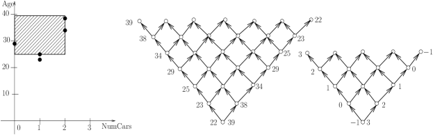
Figure 6: A maximal empty box and the two factor posets used for representing such boxes.

Let $\mathcal{F}_{\mathcal{S},k}$ be the set of all maximal $k$-boxes for a given pointset $\mathcal{S}$. Then we are interested in generating the elements of $\mathcal{F}_{\mathcal{S},k}$. Let us note that without any loss of generality, we could consider the generation of the boxes $\{B\cap D\mid B\in\mathcal{F}_{\mathcal{S},k}\}$, where $D$ is a fixed bounded box containing all points of $\mathcal{S}$ in its interior. Let us further note that the $i$th coordinate of each vertex of such a box is the same as $p_{i}$ for some $p\in\mathcal{S}$, or the $i$th coordinate of a vertex of $D$, hence all these coordinates belong to a finite set of cardinality at most $|\mathcal{S}|+2$. Thus we can view $\mathcal{F}_{\mathcal{S},k}$ as a set of boxes with vertices belonging to such a finite grid. More precisely, let $\mathcal{C}_{i}=\{p_{i}\mid p\in\mathcal{S}\}$ for $i=1,\ldots,n$ and consider the family of boxes $\mathcal{B}=\{[a,b]\subseteq\mathbb{R}^{n}\mid a,b\in\mathcal{C}_{1}\times\cdots\times\mathcal{C}_{n},~{}a\leq b\}$. For $i=1,\ldots,n$, let $u_{i}=\max\mathcal{C}_{i}$, and let $\mathcal{C}_{i}^{*}\stackrel{{\scriptstyle\mathrm{def}}}{{=}}\{u_{i}-p\mid p\in\mathcal{C}_{i}\}$ be the chain ordered in the direction opposite to $\mathcal{C}_{i}$. Consider the $2n$-dimensional box $\mathcal{C}=\mathcal{C}_{1}\times\cdots\times\mathcal{C}_{n}\times\mathcal{C}_{1}^{*}\times\cdots\times\mathcal{C}_{n}^{*}$, and let us represent every $n$-dimensional box $[a,b]\in\mathcal{B}$ as the $2n$-dimensional vector $(a,u-b)\in\mathcal{C}$, where $u=(u_{1},\ldots,u_{n})$. This gives a monotone injective mapping $\mathcal{B}\mapsto\mathcal{C}$ (not all elements of $\mathcal{C}$ define a box, since $a_{i}>b_{i}$ is possible for $(a,u-b)\in\mathcal{C}$).

It is not difficult to see that our problem reduces to solving problem GEN${}_{\mathcal{F}_{\mathcal{S},k+1}}(\mathcal{C}^{*},\mathcal{D},k+1)$, where $\mathcal{D}\stackrel{{\scriptstyle\mathrm{def}}}{{=}}\{(p,u-p)~{}:~{}p\in\mathcal{S}\}$ and we redeine support to be $S_{\mathcal{D}}(p)=\{q\in\mathcal{D}~{}:~{}q\succ p\}$ (ignoring a small number (at most $\sum_{i=1}^{n}|\mathcal{C}_{i}|$) of additionally generated elements, corresponding to non-boxes), see [KBE+07] for more details.

4.3 Minimal infrequent multi-dimensional intervals

Consider the database of intervals given in Section 2.4. An interesting observation, that may be deduced from the database, can take the form “Fewer than 40% of the customers occupy the service on Friday between 2:00-3:00 and on Saturday between 2:00-4:00”, or ”With support 60%, all customers who make full use of the service between 2:00-3:00 on Friday tend also to use the service between 2:00-3:00 on Saturday and between 1:00-2:00 on Sunday”. These examples illustrate the requirement for discovering correlations or association rules between occurrences of events over time. As in the previous examples, a fundamental problem that arises in this case is the generation of frequent and minimal infrequent multi-dimensional intervals.

More Formally, given a database of $n$-dimensional intervals $\mathcal{D}$, and $i\in[n]$, let $\mathbb{P}_{i}=\{p_{i}^{1},p_{i}^{2},\ldots,p_{i}^{k_{i}}\}$ be the set of end-points of intervals appearing in the $i$th column of $\mathcal{D}$. Clearly $k_{i}\leq 2|\mathcal{D}|$, and assuming that $p_{i}^{1}<p_{i}^{2}<\ldots<p_{i}^{k_{i}}$, we obtain a set $\mathbb{I}_{i}=\{[p_{i}^{1},p_{i}^{2}],[p_{i}^{2},p_{i}^{3}],\ldots,[p_{i}^{k_{i}-1},p_{i}^{k_{i}}]\}$ of at most $2|\mathcal{D}|$ intervals. Let $\mathcal{P}_{i}$ be the lattice of intervals defined by the set $\mathbb{I}_{i}$ (recall Definition 2), for $i=1,\ldots,n$, and let $\mathcal{P}=\mathcal{P}_{1}\times\cdots\times\mathcal{P}_{n}$. Then, each record in $\mathcal{D}$ appears as an element in $\mathcal{P}$, i.e., $\mathcal{D}\subseteq\mathcal{P}$.

Now, it is easy to see that the $t$-frequent elements of $\mathcal{P}$ are in one-to-one correspondence with the $t$-frequent intervals defined by $\mathcal{D}$, in the obvious way: if $x=(x_{1},\ldots,x_{n})\in\mathcal{P}$ is a frequent element, then the corresponding interval $(I_{1},\ldots,I_{n})$ (where $I_{i}$ corresponds to $x_{i}$, for $i=1,\ldots,n$) is the corresponding frequent interval. The situation with minimal infrequent intervals is just a bit more complicated: if $x=(x_{1},\ldots,x_{n})\in\mathcal{P}$ is a minimal infrequent element then the corresponding minimal infrequent interval $(I_{1},\ldots,I_{n})$ is computed as follows. For $i=1,\ldots,n$, if $x_{i}=l_{i}$ is the minimum element of $\mathcal{P}_{i}$, then $I_{i}=\emptyset$. If $x_{i}$ represents a point $p_{i}\in\mathbb{R}$ then $I_{i}=[p_{i},p_{i}]$. Otherwise, let $[a_{i},b_{i}]$ and $[c_{i},d_{i}]$ be the two intervals corresponding to the two immediate predecessors of $x_{i}$ in $\mathcal{P}_{i}$, where we assume $a_{i}<c_{i}$. If $a_{i}=b_{i}$ and $c_{i}=d_{i}$ then $x_{i}$ corresponds to the interval $[a_{i},c_{i}]$ and we have an infinite number of minimal infrequent intervals defined (uniquely) by $I_{i}$, namely $I_{i}=[p_{i},p_{i}]$ for all points $p_{i}$ in the open interval $(a_{i},c_{i})$. Finally, if $a_{i}<b_{i}$ and $c_{i}<d_{i}$, then $I_{i}=[c_{i}-\epsilon,b_{i}+\epsilon]$ for a sufficiently small constant $\epsilon$ (which can be taken as the smallest precision used in the representation of intervals, e.g., 1 minute). Consequently, in all cases, our problems reduce to finding $t$-frequent/minimal $t$-infrequent elements in the lattice product $\mathcal{P}$.

5 Complexity

5.1 Minimal infrequent elements

We will illustrate now that, for all the examples considered above, the problem of finding minimal $t$-infrequent elements, that is, problem GEN${}_{\mathcal{F}_{\mathcal{D},t}}(\mathcal{P},\mathcal{D},t,\mathcal{X})$ can be solved in incremental quasi-polynomial time.

Central to this is the notion of duality testing. Call two subsets $\mathcal{A},\mathcal{B}\subseteq\mathcal{P}$ partially dual if the following condition holds:

$$a\not\preceq b,~{}~{}\mbox{for all }a\in\mathcal{A},b\in\mathcal{B}.$$ (6)

For instance if $\mathcal{X}\subseteq\mathcal{F}_{\mathcal{D},t}$ and $\mathcal{Y}\subseteq{\mathcal{I}}(\mathcal{F}_{\mathcal{D},t})$ then $\mathcal{X},\mathcal{Y}$ are partially dual. The duality testing problem on $\mathcal{P}$ is the following:

DUAL$(\mathcal{P},\mathcal{A},\mathcal{B})$:

Given two partially dual sets $\mathcal{A},\mathcal{B}\subseteq\mathcal{P}$, check if there exists an element $x\in\mathcal{P}$, such that

$$x\not\succeq a a\in\mathcal{A} x\not\preceq b b\in\mathcal{B}$$ for all and for all . (7)

Let $m=|\mathcal{A}|+|\mathcal{B}|$. The main result that we need here is the following.

Theorem 2

([BEG+02, Elb])

(i) If each $\mathcal{P}_{i}$ is a chain, then DUAL$(\mathcal{P},\mathcal{A},\mathcal{B})$ can be solved in $n\cdot m^{o(\log m)}$ time.

(ii) If each $\mathcal{P}_{i}$ is tree poset, then DUAL$(\mathcal{P},\mathcal{A},\mathcal{B})$ can be solved in $\operatorname{poly}(n,\mu(\mathcal{P}))\cdot m^{o(\log m)}$ time, where $\mu(P)=\max\{|\mathcal{P}_{i}|~{}:~{}i\in[n]\}$.

(iii) If each poset $\mathcal{P}_{i}$ is a lattice of intervals then DUAL$(\mathcal{P},\mathcal{A},\mathcal{B})$ can be solved in $k^{O(\log^{2}k)}$ time, where $k=m+\sum_{i=1}^{n}|\mathcal{P}_{i}|$.

We also note that a mixture of posets of the three types can be taken in the product and the running time will be the maximum of the bounds in (i), (ii) and (iii). Thus the duality testing problem can be solved in quasi-polynomial time for the classes of posets that arise in our applications. To apply this result to the generation of minimal infrequent elements, we need another important ingredient. Namely, that the number of all maximal $t$-frequent elements is polynomially small in the number of minimal $t$-infrequent elements. In fact the following stronger bound holds.

Theorem 3 ([BGKM02])

For any poset product $\mathcal{P}=\mathcal{P}_{1}\times\ldots\times\mathcal{P}_{n}$ in which each two elements of each poset $\mathcal{P}_{i}$ have at most one join, the set $\mathcal{F}_{\mathcal{D},t}$ is uniformly dual-bounded in the sense that

$$\left|{\mathcal{I}}(\mathcal{A})\cap{\mathcal{I}}(\mathcal{F}_{\mathcal{D},t})\right|\leq(|\mathcal{D}|-t+1)|\mathcal{A}|,$$ (8)

for any non-empty subset $\mathcal{A}\subseteq\mathcal{F}_{\mathcal{D},t}$.

To generate the elements of $\mathcal{F}_{\mathcal{D},t}$ we keep two lists $\mathcal{X}\subseteq\mathcal{F}_{\mathcal{D},t}$ and $\mathcal{Y}\subseteq{\mathcal{I}}(\mathcal{F}_{\mathcal{D},t})$, both initially empty. Given these partial lists, we call the procedure for solving DUAL$(\mathcal{P},\mathcal{X},\mathcal{Y})$. If it returns an element $x$ satisfying (7), we obtain from $x$ a vector $x^{\prime}$ in $\mathcal{F}_{\mathcal{D},t}$ or ${\mathcal{I}}(\mathcal{F}_{\mathcal{D},t})$, depending respectively on whether $x$ is $t$-infrequent or $t$-frequent element. This continues until no more such elements $x$ can be returned. Clearly, if this happens then all elements of $\mathcal{P}$ have been classified to either lie above some $x\in\mathcal{X}$ or below some $x\in\mathcal{Y}$, i.e., $\mathcal{X}=\mathcal{F}_{\mathcal{D},t}$ and $\mathcal{Y}={\mathcal{I}}(\mathcal{F}_{\mathcal{D},t})$. By (8), the time needed to produce a new element of $\mathcal{F}_{\mathcal{D},t}$ is at most a factor of $|\mathcal{D}|$ times the time needed to solve problem DUAL$(\mathcal{P},\mathcal{X},\mathcal{Y})$. A Pseudo-code is shown in Figure 7.

Procedure GenerateInfrequent$(\mathcal{P},\mathcal{D},t)$:
	Input: A database $\mathcal{D}\subseteq\mathcal{P}$ and a integer threshold $t$.
	Output: The $t$-minimal infrequent elements.
1.	$\mathcal{X}\mbox{\rm:= }\emptyset$; $\mathcal{Y}\mbox{\rm:= }\emptyset$.
2.	while DUAL$(\mathcal{P},\mathcal{X},\mathcal{Y})$ returns a vector $x$
3.		If $|S_{\mathcal{D}}(x)|<t$, then
4.			$x^{\prime}\mbox{\rm:= }$ a minimal vector such that $x^{\prime}\preceq x$ and $|S_{\mathcal{D}}(x)|<t$.
5.			$\mathcal{X}\mbox{\rm:= }\mathcal{X}\cup\{x^{\prime}\}$.
6.		else
7.			$x^{\prime}\mbox{\rm:= }$ a maximal vector such that $x\preceq x^{\prime}$ and $|S_{\mathcal{D}}(x)|\geq t$
8.			$\mathcal{Y}\mbox{\rm:= }\mathcal{Y}\cup\{x^{\prime}\}$.
9.	return $\mathcal{X}$.

Figure 7: A procedure for enumerating minimal infrequent elements.

Theorem 4

Let $\mathcal{P}=\mathcal{P}_{1}\times\cdot\times\mathcal{P}_{n},$ where each $\mathcal{P}_{i}$ is either a chain, a lattice of intervals, or a meet semi-lattice tree poset. Then for any $\mathcal{D}\subseteq\mathcal{P}$, and integer $t$, problem GEN${}_{\mathcal{F}_{\mathcal{D},t}}(\mathcal{P},\mathcal{D},t)$ can be solved in incremental quasi-polynomial time.

In Appendix B, we give the dualization algorithm for meet semi-lattice tree posets. We refer the reader to [Elb] for more details and for the dualization algorithm on products of lattices of intervals.

5.2 Infrequent/frequent elements

If we are interested in finding all infrequent elements rather then the minimal ones, then the problem seems to be easier. As we have seen in the applications above, one basic step in finding association rules is enumerating all frequent elements. Those can be typically found by an Apriori-like algorithm, which we give for completeness in Appendix A. Since one can regard the problem of finding infrequent elements as of that finding frequent elements on the dual poset, we can conclude that the infrequent elements can also be found by the algorithm Apriori, and hence the problem can be solved in incremental polynomial time.

Theorem 5

Let $\mathcal{P}=\mathcal{P}_{1}\times\cdots\times\mathcal{P}_{n},$, $\mathcal{D}\subseteq\mathcal{P}$, and $t$ be an integer. Then all $t$-frequent ($t$-infrequent) elements can be computed with amortized delay.

6 Conclusion

In this chapter, we have looked at a general framework that allows us to mine associations from different types of databases. We have argued that the rules obtained under this framework are generally stronger than the ones obtained from techniques that use binarization. A fundamental problem that comes out from this framework is that of finding minimal infrequent elements in a given product of partially ordered sets. As we have seen, this problem can be solved in quasi-polynomial time, while the problem becomes easier if we are interested in finding all infrequent/frequent elements. On the theoretical level, while the complexity of enumerating minimal infrequent elements is not known to be polynomial, the problem is unlikely to be NP-hard unless every NP-complete problem can be solved in quasi-polynomial time.

Finally, we mention that a number of implementations exist for the duality testing problem on products of chains [BMR03, KS05, KBEG06], and for the generation of infrequent elements [KBEG06] on such products. Experiments in [KBEG06] indicate that the algorithms behave practically much faster than the theoretically best-known upper bounds on their running times, and therefore may be applicable in practical applications. Improving these implementations further and putting them into practical use, as well as the extension to more general products of partially ordered sets remain challenging issues that can be the subject of interesting future research.

Appendix A: Frequent elements generation - Apriori algorithm

Let $\mathcal{P}=\mathcal{P}_{1}\times\cdots\times\mathcal{P}_{n}$ be a product of $n$ posets and $\mathcal{D}\subseteq\mathcal{P}$ be a database. For simplicity, we assume that $\mathcal{P}$ has a minimum element $l=(l_{1},\ldots,l_{n})$. Given an integer threshold $t$, we present below an Apriori-like algorithm that finds all the $t$-frequent elements $x\in\mathcal{P}$. This can be viewed as a strict generalization of the one for frequent itemsets in [AS94]. The algorithm for generating all infrequent elements is exactly the same, but it should work on the dual poset $\mathcal{P}^{*}$. We assume that, for $i=1,\ldots,n$, each element in $x\in\mathcal{L}_{i}$ is assigned a number $d(x)$ that indicates the longest distance, in the precedence graph of $\mathcal{P}_{i}$, from the smallest element $l_{i}$ of $\mathcal{L}_{i}$ to $x$ (such numbers are easy to compute since the precedence graph is acyclic). For $x=(x_{1},\ldots,x_{n})\in\mathcal{P}$, we let $d(x)=\sum_{i=1}^{n}d(x_{i})$. We say that $x$ has level $k$ is $d(x)=k$.

For $x\in\mathcal{P}_{i}$, denote by $x^{\bot}$ the set of immediate predecessors of $x$, i.e.,

$$x^{\bot}=\{y\in\mathcal{P}_{i}~{}|~{}y\prec x,~{}(\nexists z\in\mathcal{P}_{i}:y\prec z\prec x)\}.$$

Similarly, denote by $x^{\top}$ the set of immediate successors of $x$. Note that, given $x=(x_{1},\ldots,x_{n})\in\mathcal{P}$, the immediate predecessors of $x$ are given by: $x^{\bot}=\{y\in\mathcal{P}~{}|~{}y_{i}\in x_{i}^{\bot}\mbox{ for some }i\in[n]\mbox{ and }x_{j}=y_{j}\mbox{ for all }j\neq i\},$ and let $\operatorname{d^{\bot}}(\mathcal{P})=\max\{|x^{\bot}|:~{}x\in\mathcal{P}\}$. The immediate successors of $x$ are similarly defined, and we let $\operatorname{d^{\top}}(\mathcal{P})=\max\{|x^{\top}|:~{}x\in\mathcal{P}\}$. Thus $|x^{\bot}|=\sum_{i=1}^{n}|x_{i}^{\bot}|$ and $|x^{\top}|=\sum_{i=1}^{n}|x_{i}^{\top}|$, for any $x=(x_{1},\ldots,x_{n})\in\mathcal{P}$.

As in the standard Apriori algorithm for finding frequent sets, the levelwise procedure proceeds bottom-up on the levels of the poset preforming two basic steps at each level $k$: Candidate generation and pruning. In the first step, we generate a set of $\mathcal{C}$ of candidate frequent elements at level $k$, based on the set $\mathcal{F}_{k-1}$ of frequent elements that we have already produced level $k-1$. In the pruning step, this set of candidates is scanned keeping only the set if frequent elements. The procedures are shown in Figures 8-10.

Procedure Ariori$(\mathcal{P},\mathcal{D},t)$:
	Input: A database $\mathcal{D}\subseteq\mathcal{P}$ and a integer threshold $t$.
	Output: The $t$-frequent elements.
1.	$k\leftarrow 0$; $\mathcal{F}_{k}\leftarrow\{l\}$;
2.	while $\mathcal{F}_{k}\neq\emptyset$ do
3.		$\mathcal{C}\leftarrow$ Candidates($\mathcal{F}_{k},k$);
4.		$\mathcal{F}_{k+1}\leftarrow$ Prune($\mathcal{C},\mathcal{D},t$);
5.		$k\leftarrow k+1$;
6.	end
7.	return $\bigcup_{j=1}^{k}\mathcal{F}_{j}$;

Figure 8: A procedure for enumerating frequent elements.

Procedure Candidates$(\mathcal{P},\mathcal{F}_{k},k)$:
	Input: A poset $\mathcal{P}$, an integer $k$ and a set of frequent elements at level $k$.
	Output: A set of candidate frequent elements at level $k+1$.
1.	$\mathcal{C}\leftarrow\emptyset$;
2.	for all $x\in\mathcal{F}_{k}$ do
3.		for all $y\in x^{\top}$ such that $d(y)=k+1$ do
4.			if $\forall z\in y^{\bot}$ such that $d(z)=k$: $z\in\mathcal{F}_{k}$, then
5.				$\mathcal{C}\leftarrow\mathcal{C}\cup\{y\}$;
6.	return $\mathcal{C}$;

Figure 9: A procedure for level $(k+1)$-candidate generation.

Procedure Prune$(\mathcal{C},\mathcal{D},t)$:
	Input: A database $\mathcal{D}\subseteq\mathcal{P}$, a integer threshold $t$, and a set of level $k$-candidates.
	Output: The $t$-frequent elements among $\mathcal{C}$.
1. $\mathcal{F}\leftarrow\emptyset$;
2.	for all $x\in\mathcal{C}$ do
3.		if $|S_{\mathcal{D}}(x)|\geq t$ then
4.			$\mathcal{F}\leftarrow\mathcal{F}\cup\{x\}$;
5.	return $\mathcal{F}$;

Figure 10: A procedure for extracting frequent elements from candidates.

Clearly, the number of scans of the database can be reduced by computing the contribution of each transaction to the counts of all candidates before reading the next transaction, see e.g. [AS94].

Let $\tau$ be the maximum time required by the procedure to compute the value of the function $|S_{\mathcal{D}}(x)|$ for any $x\in\mathcal{P}$.

Lemma 1

Algorithm Apriori outputs all $t$-frequent elements of $\mathcal{P}$, with amortized delay $O(\operatorname{d^{\bot}}(\mathcal{P})\operatorname{d^{\top}}(\mathcal{P})(n\sum_{i=0}^{n}\log|\mathcal{P}_{i}|+\tau))$.

Proof. Let us note by induction on $k=0,1,\ldots$, that $\mathcal{F}_{k}=\mathcal{F}_{k}^{\prime}\stackrel{{\scriptstyle\mathrm{def}}}{{=}}\{x\in\mathcal{P}~{}:~{}d(x)=k,|S_{\mathcal{D}}(x)|\geq t\}$. Indeed, this holds initially for $k=0$. Assume that it also holds for any $k>0$, and consider the set $\mathcal{F}_{k+1}$ generated in Step 4 of procedure Apriori$(\mathcal{P},\mathcal{D},t)$. From Steps 3 in procedure Candidates$(\mathcal{P},\mathcal{F}_{k},k)$ and 3 in Prune$(\mathcal{C},\mathcal{D},t)$, we note that $\mathcal{F}_{k+1}\subseteq\mathcal{F}_{k+1}^{\prime}$. So it remains to show that $\mathcal{F}_{k+1}^{\prime}\subseteq\mathcal{F}_{k+1}$. For this consider any $y\in\mathcal{F}_{k+1}^{\prime}$ and observe, by the anti-monotonicity of $|S_{\mathcal{D}}(\cdot)|$ and the definition of $d(\cdot)$, that there exists an $x\in\mathcal{F}_{k}^{\prime}=\mathcal{F}_{k}$ such that $y\in x^{\top}$. Thus $x$ and $y$ pass respectively the tests in Steps 2 and 3 of procedure Candidates$(\mathcal{F}_{k},k)$. Moreover, every $z\in y^{\bot}$ with $d(z)=k$ belongs to $\mathcal{F}_{k}^{\prime}$ and hence to $\mathcal{F}_{k}$ and therefore $y$ will be added to the list of candidates $\mathcal{C}$ in procedure Candidates$(\mathcal{F}_{k},k)$ and to the frontier list $\mathcal{F}_{k+1}$ in Step 4 of procedure Prune$(\mathcal{C},\mathcal{D},t)$.

Now we consider the running time of the procedure. Let $k_{max}=\max\{k\in\mathbb{Z}_{+}~{}|~{}\mathcal{F}_{k}\neq\emptyset\}$. By implementing a balanced binary search tree on the elements of $\mathcal{F}_{k}$ (sorted according to some lexicographic ordering), we can perform the check $z\in\mathcal{F}_{k}$, for any $z\in\mathcal{P}$, in $O(n\log|\mathcal{F}_{k}|)$ time. Thus it follows that the total time required by the procedure to output the union $\mathcal{F}_{1}\cup\ldots\cup\mathcal{F}_{k_{max}}$ is bounded by

$$\sum_{k=0}^{k_{max}}\left(\sum_{x\in\mathcal{F}_{k}}\sum_{y\in x^{\top}}\left(\sum_{z\in y^{\bot}}O(n\log|\mathcal{F}_{k}|)+\tau\right)\right)\leq\operatorname{d^{\top}}(\mathcal{P})\operatorname{d^{\bot}}(\mathcal{P})\sum_{k=0}^{k_{max}}|\mathcal{F}_{k}|(O(n\log|\mathcal{F}_{k}|)+\tau).$$

This amounts to an amortized time of

$$\operatorname{d^{\bot}}(\mathcal{P})\operatorname{d^{\top}}(\mathcal{P})\frac{\sum_{k=0}^{k_{max}}|\mathcal{F}_{k}|(O(n\log|\mathcal{F}_{k}|)+\tau)}{\sum_{k=0}^{k_{max}}|\mathcal{F}_{k}|}=\operatorname{d^{\bot}}(\mathcal{P})\operatorname{d^{\top}}(\mathcal{P})O(n\log(\sum_{k=0}^{k_{max}}|\mathcal{F}_{k}|)+\tau).$$

Note that $\sum_{k=0}^{k_{max}}|\mathcal{F}_{k}|\leq|\mathcal{P}|=\prod_{i=1}^{n}|\mathcal{P}_{i}|$, and the lemma follows. $\square$

Appendix B: Dualization in products of meet semi-lattice tree posets

Let $\mathcal{P}=\mathcal{P}_{1}\times\cdots\times\mathcal{P}_{n}$, where the precedence graph of each poset $\mathcal{P}_{i}$ is a meet semi-lattice tree poset (henceforth abbreviated MSTP), and let $\mathcal{A},\mathcal{B}\subseteq\mathcal{P}$ two antichains satisfying (6). We say that $\mathcal{B}$ is dual to $\mathcal{A}$ if $\mathcal{B}={\mathcal{I}}(\mathcal{A})$.

Note that in this case, we have the following decomposition of $\mathcal{P}$

$$\mathcal{A}^{+}\cap\mathcal{B}^{-}=\emptyset,~{}~{}~{}~{}\mathcal{A}^{+}\cup\mathcal{B}^{-}=\mathcal{P},$$ (9)

and thus problem DUAL$(\mathcal{P},\mathcal{A},\mathcal{B})$ can be equivalently stated as follows:

DUAL$(\mathcal{P},\mathcal{A},\mathcal{B})$:

Given antichains $\mathcal{A},\mathcal{B}\subseteq\mathcal{P}$ satisfying (6), check if there an $x\in\mathcal{P}\setminus(\mathcal{A}^{+}\cup\mathcal{B}^{-})$.

Given any $\mathcal{Q}\subseteq\mathcal{P}$, let us denote by

$$\mathcal{A}(\mathcal{Q})=\{a\in\mathcal{A}~{}|~{}a^{+}\cap\mathcal{Q}\neq\emptyset\},~{}~{}~{}~{}~{}~{}~{}\mathcal{B}(\mathcal{Q})=\{b\in\mathcal{B}~{}|~{}b^{-}\cap\mathcal{Q}\neq\emptyset\}.$$

These are the effective subsets of $\mathcal{A},\mathcal{B}$ that play a role in problem DUAL$(\mathcal{Q},\mathcal{A},\mathcal{B})$. Note that, for $a\in\mathcal{A}$ and $\mathcal{Q}=\mathcal{Q}_{1}\times\ldots\times\mathcal{Q}_{n}$, $a^{+}\cap\mathcal{Q}\neq\emptyset$ if and only if $a_{i}^{+}\cap\mathcal{Q}_{i}\neq\emptyset$, for all $i\in[n]$. Thus, the sets $\mathcal{A}(\mathcal{Q})$ and $\mathcal{B}(\mathcal{Q})$ can be found in $O(nm\mu(\mathcal{P}))$ time.

To solve problem DUAL$(\mathcal{P},\mathcal{A},\mathcal{B})$, we decompose it into a number of smaller subproblems which are solved recursively. In each such subproblem, we start with a subposet $\mathcal{Q}=\mathcal{Q}_{1}\times\ldots\times\mathcal{Q}_{n}\subseteq\mathcal{P}$ (initially $\mathcal{Q}=\mathcal{P}$), and two subsets $\mathcal{A}(\mathcal{Q})\subseteq\mathcal{A}$ and $\mathcal{B}(\mathcal{Q})\subseteq\mathcal{B}$, and we want to check whether $\mathcal{A}(\mathcal{Q})$ and $\mathcal{B}(\mathcal{Q})$ are dual in $\mathcal{Q}$. The decomposition of $\mathcal{Q}$ is done by decomposing one factor poset, say $\mathcal{Q}_{i},$ into a number of (not necessarily disjoint) subposets $\mathcal{Q}_{i}^{1},\ldots,\mathcal{Q}_{i}^{r},$ and solving $r$ subproblems on the $r$ different posets $\mathcal{Q}_{1}\times\cdots\times\mathcal{Q}_{i-1}\times\mathcal{Q}_{i}^{j}\times\mathcal{Q}_{i+1}\times\cdots\times\mathcal{Q}_{n},$ $j=1,\ldots,r$. For brevity, let us denote by $\overline{\mathcal{Q}}$ the product $\mathcal{Q}_{1}\times\cdots\times\mathcal{Q}_{i-1}\times\mathcal{Q}_{i+1}\times\cdots\times\mathcal{Q}_{n},$, and accordingly by $\overline{q}$ the element $(q_{1},\ldots,q_{i-1},q_{i+1},\ldots,q_{n})$, for an element $q=(q_{1},q_{2},\ldots,q_{n})\in\mathcal{Q}$.

The algorithm is shown in Figure 6. We assume that procedure $\operatorname{TD}$ returns either true or false depending on whether $\mathcal{A}$ and $\mathcal{B}$ are dual in $\mathcal{Q}$ or not. Returning an element $x\in\mathcal{Q}\setminus(\mathcal{A}^{+}\cup\mathcal{B}^{-})$ in the latter case is straightforward, as it can be obtained from any subproblem that failed the test for duality.

Note that after decomposing one of the posets, some elements $x\in\mathcal{A}\cup\mathcal{B}$ do not belong to the current poset $\mathcal{Q}$. In step 1, the elements that do not affect the solution are deleted, while in step 2, those that affect the solution are projected down to the current poset $\mathcal{Q}$ (by replacing each $a\in\mathcal{A}$ ($b\in\mathcal{B}$) with unique element above $a$ (respectively, below $b$) in $\mathcal{Q}$.) In step 3, we check if the size of the problem is sufficiently small, and if so we use an exhaustive search procedure to decide the duality of $\mathcal{A}$ and $\mathcal{B}$ in $\mathcal{Q}$.

Starting from step 5, we decompose $\mathcal{Q}\subseteq\mathcal{P}$ by picking $a\in\mathcal{A}$, $b\in\mathcal{B}$ and an $i\in[n]$, such that $a_{i}\not\preceq b_{i}$. The algorithm uses the effective volume $v=v(\mathcal{A},\mathcal{B})$ to compute the threshold

$$\epsilon(v)=\frac{1}{\chi(v)},~{}~{}~{}~{}\mbox{ where}~{}\chi(v)^{\chi(v)}=v\stackrel{{\scriptstyle\mathrm{def}}}{{=}}|\mathcal{A}||\mathcal{B}|.$$

If the minimum of $\epsilon^{\mathcal{A}}\stackrel{{\scriptstyle\mathrm{def}}}{{=}}|\mathcal{A}_{\succeq}(a_{i})|/|\mathcal{A}|$ and $\epsilon^{\mathcal{B}}\stackrel{{\scriptstyle\mathrm{def}}}{{=}}|\mathcal{B}_{\not\succeq}(a_{i})|/|\mathcal{B}|$, where $\mathcal{A}_{\succeq}(a_{i})\stackrel{{\scriptstyle\mathrm{def}}}{{=}}\{x\in\mathcal{A}:x_{i}\succeq a_{i}\}$ and $\mathcal{B}_{\not\succeq}(a_{i})\stackrel{{\scriptstyle\mathrm{def}}}{{=}}\{x\in\mathcal{B}:x_{i}\not\succeq a_{i}\}$, is bigger than $\epsilon(v)$, then we decompose $\mathcal{Q}_{i}$ into two MSTP’s $\mathcal{Q}_{i}^{\prime}\leftarrow\mathcal{Q}_{i}\cap a_{i}^{+}$ and $\mathcal{Q}_{i}^{\prime\prime}\leftarrow\mathcal{Q}_{i}\setminus\mathcal{Q}_{i}^{\prime},$ and solve recursively two problems on these posets (steps 8 and 9).

Otherwise we proceed as follows. For $x\in\mathcal{Q}_{i}$ denote by $p(x)$ the unique predecessor of $x$ in $\mathcal{Q}_{i}$. Let $\mathcal{Q}_{i}^{0}=p(a_{i})^{-}\cap\mathcal{Q}_{i}^{\prime\prime}$, $\mathcal{Q}_{i}^{1}=\mathcal{Q}_{i}^{\prime},$ and $\mathcal{Q}_{i}^{2},\ldots,\mathcal{Q}_{i}^{r}$ be the MSTP’s obtained by deleting $p(a_{i})^{-}$ from $\mathcal{Q}_{i}^{\prime\prime}$ (see Figure 11). Then we can use the decomposition in step 12.

Finally, if $\epsilon^{\mathcal{A}}\leq\epsilon(v)<\epsilon^{\mathcal{B}}$, we proceed as in steps 14-17: we solve the subproblem on $\mathcal{Q}_{i}^{\prime\prime}\times\overline{\mathcal{Q}}$, and if it does not have a solution $x$, then we process the elements $x^{1},\ldots,x^{k}$ of $\mathcal{Q}_{i}^{\prime}$ in topological order (that is, $x^{j}\prec x^{r}$ implies $j<r$). For each such element, we solve at most $|\mathcal{B}|$ subproblems on $\{x^{j}\}\times(\overline{\mathcal{Q}}\cap\overline{b}^{-})$, for $b\in\mathcal{B}_{\succeq}(p(x^{j}))$.

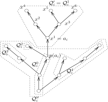
Figure 11: Decomposing the forest $\mathcal{Q}_{i}$.

Procedure $\operatorname{TD}(\mathcal{Q},\mathcal{A},\mathcal{B})$:
	Input: A subposet of a product of trees $\mathcal{Q}=\mathcal{Q}_{1}\times\cdots\times\mathcal{Q}_{n}\subseteq\mathcal{P}$ and two anti-chains $\mathcal{A},\mathcal{B}\subseteq\mathcal{P}$
	Output: true if $\mathcal{A}$ and $\mathcal{B}$ are dual in $\mathcal{Q}$ and false otherwise
1.	$\mathcal{A}\leftarrow\mathcal{A}(\mathcal{Q})$, $\mathcal{B}\leftarrow\mathcal{B}(\mathcal{Q})$
2.	$\mathcal{A}\leftarrow\operatorname{PROJECT}(\mathcal{Q},\mathcal{A})$, $\mathcal{B}\leftarrow\operatorname{PROJECT}(\mathcal{Q},\mathcal{B})$
3.	if $\min\{|\mathcal{A}|,|\mathcal{B}|\}\leq 3$ then
4.		return $\operatorname{POLY-DUAL}(\mathcal{Q},\mathcal{A},\mathcal{B})$
5.	Let $a\in\mathcal{A}$, $b\in\mathcal{B}$, and $i\in[n]$ be such that $a_{i}\not\preceq b_{i}$
6.	$\epsilon^{\mathcal{A}}\leftarrow\frac{|\mathcal{A}_{\succeq}(a_{i})|}{|\mathcal{A}|}$ and $\epsilon^{\mathcal{B}}\leftarrow\frac{|\mathcal{B}_{\not\succeq}(a_{i})|}{|\mathcal{B}|}$
7.	Let $\mathcal{Q}_{i}^{\prime}\leftarrow\mathcal{Q}_{i}\cap a_{i}^{+},$ $\mathcal{Q}_{i}^{\prime\prime}\leftarrow\mathcal{Q}_{i}\setminus\mathcal{Q}_{i}^{\prime}$
8.	if $\min\{\epsilon^{\mathcal{A}},\epsilon^{\mathcal{B}}\}>\epsilon(v(\mathcal{A},\mathcal{B}))$ then
9.		return $\operatorname{TD}(\mathcal{Q}_{i}^{\prime}\times\overline{\mathcal{Q}},\mathcal{A},\mathcal{B})\wedge\operatorname{TD}(\mathcal{Q}_{i}^{\prime\prime}\times\overline{\mathcal{Q}},\mathcal{A},\mathcal{B})$
10.	if $\epsilon^{\mathcal{B}}\leq\epsilon(v(\mathcal{A},\mathcal{B}))$ then
11.		Let $\mathcal{Q}_{i}^{0}=p(a_{i})^{-}\cap\mathcal{Q}_{i}^{\prime\prime}$, $\mathcal{Q}_{i}^{1},\ldots,\mathcal{Q}_{i}^{r}$ be the MSTP’s composing $\mathcal{Q}_{i}\setminus\mathcal{Q}_{i}^{0}$
12.		return $\bigwedge_{j=1}^{r}\operatorname{TD}(\mathcal{Q}_{i}^{j}\times\overline{\mathcal{Q}},\mathcal{A},\mathcal{B})\wedge(\bigwedge_{a\in\mathcal{A}_{\preceq}(a_{i})}\operatorname{TD}(\mathcal{Q}_{i}^{0}\times(\overline{\mathcal{Q}}\cap\overline{a}^{+}),\mathcal{A},\mathcal{B}))$
13.	else
14.		Let $x^{1},\ldots,x^{k}$ be the elements of $\mathcal{Q}_{i}^{\prime}$ in topologically non-decreasing order
15.		$d\leftarrow\operatorname{TD}(\mathcal{Q}_{i}^{\prime\prime}\times\overline{\mathcal{Q}},\mathcal{A},\mathcal{B})$
16.		for $i=1,\ldots,k$ do
17.			$d\leftarrow d\wedge(\bigwedge_{b\in\mathcal{B}_{\succeq}(p(x^{j}))}\operatorname{TD}(\{x^{j}\}\times(\overline{\mathcal{Q}}\cap\overline{b}^{-}),\mathcal{A},\mathcal{B}))$
18.		return $d$

Figure 12: The dualization procedure for MSTP’s.

References

- [AIS93] R. Agrawal, T. Imieliński, and A. Swami. Mining association rules between sets of items in large databases. In SIGMOD ’93: Proceedings of the 1993 ACM SIGMOD international conference on Management of data, pages 207–216, New York, NY, USA, 1993. ACM.
- [AMS+96] R. Agrawal, H. Mannila, R. Srikant, H. Toivonen, and A. I. Verkamo. Fast discovery of association rules. pages 307–328, 1996.
- [AS94] R. Agrawal and R. Srikant. Fast algorithms for mining association rules in large databases. In VLDB ’94: Proceedings of the 20th International Conference on Very Large Data Bases, pages 487–499, San Francisco, CA, USA, 1994. Morgan Kaufmann Publishers Inc.
- [AZ04] M.-L. Antonie and O. R. Zaïane. Mining positive and negative association rules: An approach for confined rules. In PKDD, pages 27–38, 2004.
- [BEG+02] E. Boros, K. Elbassioni, V. Gurvich, L. Khachiyan, and K. Makino. Dual-bounded generating problems: All minimal integer solutions for a monotone system of linear inequalities. SIAM Journal on Computing, 31(5):1624–1643, 2002.
- [BGKM02] E. Boros, V. Gurvich, L. Khachiyan, and K. Makino. On the complexity of generating maximal frequent and minimal infrequent sets. In STACS ’02: Proceedings of the 19th Annual Symposium on Theoretical Aspects of Computer Science, pages 133–141, London, UK, 2002. Springer-Verlag.
- [BGKM03] E. Boros, V. Gurvich, L. Khachiyan, and K. Makino. On maximal frequent and minimal infrequent sets in binary matrices. Ann. Math. Artif. Intell., 39(3):211–221, 2003.
- [BLQ98] L.-F. Mun B. Liu, K. Wang and X.-Z. Qi. Using decision tree induction for discovering holes in data. In PRICAI ’98: Proceedings of the 5th Pacific Rim International Conference on Artificial Intelligence, pages 182–193, London, UK, 1998. Springer-Verlag.
- [BMR03] J. Bailey, T. Manoukian, and K. Ramamohanarao. A fast algorithm for computing hypergraph transversals and its application in mining emerging patterns. In ICDM, pages 485–488, 2003.
- [BMS97] S. Brin, R. Motwani, and C. Silverstein. Beyond market baskets: generalizing association rules to correlations. In SIGMOD ’97: Proceedings of the 1997 ACM SIGMOD international conference on Management of data, pages 265–276, New York, NY, USA, 1997. ACM.
- [EGLM01] J. Edmonds, J. Gryz, D. Liang, and R. J. Miller. Mining for empty rectangles in large data sets. In ICDT, pages 174–188, 2001.
- [Elb] K. Elbassioni. Algorithms for dualization over products of partially ordered sets, to appear. SIAM J. Disctere Math.
- [GMKT97] D. Gunopulos, H. Mannila, R. Khardon, and H. Toivonen. Data mining, hypergraph transversals, and machine learning (extended abstract). In PODS ’97: Proceedings of the 16th ACM SIGACT-SIGMOD-SIGART symposium on Principles of database systems, pages 209–216, New York, NY, USA, 1997. ACM Press.
- [HCC93] J. Han, Y. Cai, and N. Cercone. Data-driven discovery of quantitative rules in relational databases. IEEE Transactions on Knowledge and Data Engineering, 05(1):29–40, 1993.
- [HF95] J. Han and Y. Fu. Discovery of multiple-level association rules from large databases. In VLDB ’95: Proceedings of the 21th International Conference on Very Large Data Bases, pages 420–431, San Francisco, CA, USA, 1995. Morgan Kaufmann Publishers Inc.
- [HMWG98] J. Hipp, A. Myka, R. Wirth, and U. Güntzer. A new algorithm for faster mining of generalized association rules. In PKDD, pages 74–82, 1998.
- [HW02] Y.-F. Huang and C.-M. Wu. Mining generalized association rules using pruning techniques. In ICDM, pages 227–234, 2002.
- [KBE+07] L. Khachiyan, E. Boros, K. Elbassioni, V. Gurvich, and K. Makino. Dual-bounded generating problems: Efficient and inefficient points for discrete probability distributions and sparse boxes for multidimensional data. Theor. Comput. Sci., 379(3):361–376, 2007.
- [KBEG06] L. Khachiyan, E. Boros, K. Elbassioni, and V. Gurvich. An efficient implementation of a quasi-polynomial algorithm for generating hypergraph transversals and its application in joint generation. Discrete Applied Mathematics, 154(16):2350–2372, 2006.
- [Koh08] Y. S. Koh. Mining non-coincidental rules without a user defined support threshold. In PAKDD, pages 910–915, 2008.
- [KP07] Y. S. Koh and R. Pears. Efficiently finding negative association rules without support threshold. In Australian Conference on Artificial Intelligence, pages 710–714, 2007.
- [KS05] D. J. Kavvadias and E. C. Stavropoulos. An efficient algorithm for the transversal hypergraph generation. J. Graph Algorithms Appl., 9(2):239–264, 2005.
- [LHM99] B. Liu, W. Hsu, and Y. Ma. Mining association rules with multiple minimum supports. In KDD ’99: Proceedings of the fifth ACM SIGKDD international conference on Knowledge discovery and data mining, pages 337–341, New York, NY, USA, 1999. ACM.
- [Lin03] J.-L. Lin. Mining maximal frequent intervals. In SAC ’03: Proceedings of the 2003 ACM symposium on Applied computing, pages 426–431, New York, NY, USA, 2003. ACM.
- [LKH97] B. Liu, L.-P. Ku, and Wynne Hsu. Discovering interesting holes in data. In IJCAI (2), pages 930–935, 1997.
- [Man98] H. Mannila. Database methods for data mining, tutorial. In KDD ’98: Proceedings of the fifth ACM SIGKDD international conference on Knowledge discovery and data mining. ACM, 1998.
- [MNE+06] M. D. Mustafa, N. F. Nabila, D. J. Evans, M. Y. Saman, and A. Mamat. Association rules on significant rare data using second support. Int. J. Comput. Math., 83(1):69–80, 2006.
- [NCJK01] A. A. Nanavati, K. P. Chitrapura, S. Joshi, and R. Krishnapuram. Mining generalised disjunctive association rules. In CIKM ’01: Proceedings of the tenth international conference on Information and knowledge management, pages 482–489, New York, NY, USA, 2001. ACM.
- [SA95] R. Srikant and R. Agrawal. Mining generalized association rules. In VLDB ’95: Proceedings of the 21th International Conference on Very Large Data Bases, pages 407–419, San Francisco, CA, USA, 1995. Morgan Kaufmann Publishers Inc.
- [SA96] R. Srikant and R. Agrawal. Mining quantitative association rules in large relational tables. In SIGMOD ’96: Proceedings of the 1996 ACM SIGMOD international conference on Management of data, pages 1–12, New York, NY, USA, 1996. ACM.
- [Sch03] B. S. W. Schröder. Ordered Sets: An Introduction. Birkhäuser, Boston, 2003.
- [SVTV05] L. K. Sharma, O. P. Vyas, U. S. Tiwary, and R. Vyas. A novel approach of multilevel positive and negative association rule mining for spatial databases. In MLDM, pages 620–629, 2005.
- [TS98] S. Thomas and S. Sarawagi. Mining generalized association rules and sequential patterns using sql queries. In KDD, pages 344–348, 1998.
- [TYZ05] Q. Tong, B. Yan, and Y. Zhou. Mining quantitative association rules on overlapped intervals. In ADMA, pages 43–50, 2005.
- [YBYZ02] X. Yuan, B .P. Buckles, Z. Yuan, and J. Zhang. Mining negative association rules. Computers and Communications, IEEE Symposium on, 0:623, 2002.
- [Zak00] M. J. Zaki. Generating non-redundant association rules. In KDD, pages 34–43, 2000.