Core-Periphery in Networks: An Axiomatic Approach

Recent evidence shows that in many societies worldwide the relative sizes of the economic and social elites are continuously shrinking. Is this a natural social phenomenon? What are the forces that shape this process? We try to address these questions by studying a Core-Periphery social structure composed of a social elite, namely, a relatively small but well-connected and highly influential group of powerful individuals, and the rest of society, the periphery. Herein, we present a novel axiom-based model for the forces governing the mutual influences between the elite and the periphery. Assuming a simple set of axioms, capturing the elite’s dominance, robustness, compactness and density, we are able to draw strong conclusions about the elite-periphery structure. In particular, we show that a balance of powers between elite and periphery and an elite size that is sub-linear in the network size are universal properties of elites in social networks that satisfy our axioms. We note that the latter is in controversy to the common belief that the elite size converges to a linear fraction of society (most recently claimed to be $1\%$). We accompany these findings with a large scale empirical study on about $100$ real-world networks, which supports our results.

1 Introduction

In his book Mind and Society [24], Vilfredo Pareto wrote what is by now widely accepted by sociologists: “Every people is governed by an elite, by a chosen element of the population”. Indeed, with the exception of some rare examples of utopian or totally egalitarian societies, almost all societies exhibit an (often radically) uneven distribution of power, influence and wealth among their members, and, in particular, between the elite and its complement, often called the periphery or the masses. Typically, the elite is small, powerful and influential and the periphery is larger, less organized and less dominant. This division is usually referred to as a core-periphery partition [4] and the problem of identifying this partition has recently received increased interest [26, 32, 16]. However, while the core-periphery structure is perhaps the most high-level structure of society, it has so far not received a satisfactory quantitative definition. In fact, it seems unlikely that a single formal definition exists that suits all elite types in all social networks. Moreover, it is not clear that the elite must be unique.

To illustrate this last point, let us consider the following mental experiment. Sort the members of society by decreasing order of influence, and add them to a set $\mathcal{E}$ (representing the intended elite) one by one in this order. After the first step, $\mathcal{E}$ contains only one member of society, albeit the most influential one, hence clearly it cannot yet be thought of as “the elite” - it simply has insufficient power. This holds true also for the next few sets obtained in this way. On the other extreme, if the process is continued to its conclusion, we end up with $\mathcal{E}$ containing the entire society, which is clearly too large to be considered “the elite”. The question is therefore: at which point along this process does $\mathcal{E}$ qualify as an elite?

Intuitively, the “break-point” where the process should be halted is the point where adding new members into $\mathcal{E}$ no longer serves to significantly strengthen the group but rather “dilutes” its power (relative to its size). This point is not well-defined, and depends to some extent on the specific circumstances of the society. In this paper we propose a concrete choice for this break-point, referred to as the power symmetry point of the elite. The core and periphery are at their power symmetry point if the overall influence of the elite (nearly) equals that of the periphery.

	(b)	(c)
(a)	(d)	(e)

Figure 1: Illustration of concepts via a fictional example using the social network of Marvel’s superheroes. There is a link between two heroes if they appeared together in many comic books [1]. (a) The network of the most highly connected 139 Marvel’s superheroes and the 924 links between them, partitioned into a core (red vertices with red internal edges) and a periphery (green vertices with green internal edges). Blue edges are “crossing” edges, connecting core and periphery vertices. (b) The (dense) core subgraph (27 vertices, 252 edges). (c) The (sparser) periphery subgraph (112 vertices, 249 edges). (d) A representation of the elite-periphery partition in the form of the adjacency matrix of the network (cf. [6]). (e) The elite influence shift diagram, based on adding the 139 vertices to the elite in order of their degree.

Our main contribution is a characterization of elites, i.e., a set of properties (formulated as “axioms”) that any definition for an elite must adhere to. While this characterization does not lead to pinpointing a single definition for the elite, it narrows down the range of subsets of society that are suitable candidates to be the elite, and moreover, it is powerful enough to allow us to derive several conclusions concerning basic properties of the elite-periphery structure of society.

Let us next describe two of our main conclusions. The first result, stated in Theorem 3.1, is that elites satisfying the axioms of our model are at their power symmetry point. This implies that the power of the periphery is similar to that of the elite, or in other words, that as society evolves, the “natural” core-periphery partition maintains a balance between these two groups.

Our second conclusion applies to the size of the elite. Recent reports show that the gap between the richest people and the masses keeps increasing, and that decreasingly fewer people amass more and more wealth [13, 23]. Claims like “The top 10 percent no longer takes in one-third of our income – it now takes half,” made by President Obama [28] when recently addressing the issue, are interpreted as implying that the economic and political elites become increasingly more greedy and overbearing. Such claims are often used in order to criticize governments and regulatory financial institutions for neglecting to cope with this disturbing development. The question raised by us is: can society help it, or is this phenomenon an unavoidable by-product of some inherent natural properties of society? We claim that in fact, one can predict the shrinkage of elite size with time (as a fraction of the entire society size) based on the very nature of social elites. In particular, in our model, such shrinkage is the natural result of a combination of three facts: First, society grows. Second, elites are denser than peripheries (informally meaning that they are much better connected). Third, the size of a dense elite at the power symmetry point is sub-linear in the size of the society. Combining these facts implies that the fraction of the total population size comprised by dense elites will decrease as the population grows with time. We prove this formally in Theorem 4.2. The empirical evidence we present in this work lends additional support to the above claim.

A dual question we are interested in concerns the stable size of the elite in a growing society: How small can the elite be while still maintaining its inherent properties? We prove that under our model, an elite cannot be smaller than $\Omega(\sqrt{m})$, where $m$ is the number of network edges.

Consequently, we assert that the elite’s symmetry of powers and sublinear size properties should indeed join the growing list of universal properties of social networks established in recent years, such as short average path lengths (a.k.a. the “small world” phenomenon), high clustering coefficients, heavy-tailed degree distributions (e.g., scale-free networks), navigability, and more recently dynamic properties such as densification and a shrinking diameter [29, 2, 18, 21].

As a small illustrative example for the meaning of our terms we consider, in Figure 1 (a)-(c), the network of top 139 Marvel’s superheroes and the 924 links interconnecting them (where two heroes are connected by a link if they appeared together in a story) [1]. We partitioned this network into a core and a periphery as shown by the colors in Figure 1(a). Several striking features can be clearly observed in this figure. First, the core (containing, e.g., Captain America ,Spiderman and Thor) is dense and organized while the periphery is much sparser and less structured. Second, despite their considerable size difference, both the elite and the periphery have almost the same number of internal edges ($\approx 250$), thus exhibiting what we refer to as a symmetry of powers. Third, the number of “crossing” edges connecting the core to the periphery is almost twice as large (425), reaching most of the vertices in the periphery. Last, the size of the core is “only” 27 vertices (with 112 vertices in the periphery). We argue, and support by evidence, that it makes sense to consider 27 as about $\sqrt{924}$, and more generally, view the core size as roughly the square root of the number of edges in the network. For almost all networks, a core of size about $\sqrt{m}$ (where $m$ is the number of edges) will not grow as a linear fraction of the number of vertices.

The rest of the paper is organized as follows. Section 2 presents our model of influence and axioms. Section 3 discusses the property of power symmetry (Appendix B expands on power symmetry in random graphs.) In Section 4 we analyze the size properties of the elite. Section 5 presents our empirical results. Related work is provided in Section 6, and finally, we conclude with a discussion in Section 7.

2 An Axiomatic Approach

The conceptual approach we adopt towards studying core-periphery properties diverges from the established traditions in the field of social networks. The common approach to explaining empirical results on social networks is based on providing a new concrete (usually random) evolutionary model and comparing its predictions to the observed data. In contrast, we propose an axiomatic approach to the questions at hand. This approach is based on postulating a small set of axioms, capturing certain expectations about the network structure and the basic properties that an elite must exhibit in order to maintain its power in the society. Two main advantages of the axiomatic approach are that a suitable set of axioms attaches an “interpretation” or “semantics” to observed phenomena, and moreover, once agreeing on the axioms, it becomes possible to draw conclusions using logical arguments. For example, it may become possible to infer some information on the asymptotic behavior of a growing network, which is not always clear from empirical findings.

The framework presented here for describing the elite-periphery structure in a social network revolves around the fundamental notion of influence among groups of vertices. The underlying assumption is that the elite has more influence than the rest of the population, allowing it on the one hand to control the rest of the population, and on the other to protect its members from being controlled by others outside the elite. We refer to these two capabilities, respectively, as dominance and robustness.

2.1 Influence and Core-Periphery Partition

We consider influence to be a measurable quantity between any two (not necessarily distinct) groups of vertices $X$ and $Y$, abstractly denoted by $\mathcal{I}(X,Y)$. The groups $X$ and $Y$ do not necessarily have to be distinct, and in particular, we are also interested in the internal influence exerted by the vertices of a group $X$ on themselves, denoted $\mathcal{I}(X,X)$.

Two central strengths of an elite in a given society are its dominance on the rest of society on the one hand, and its resistance to influence by the rest of society on the other. We will quantify these two aspects shortly. Denote the elite by a set $\mathcal{E}$ and the rest of society (the “periphery”) by $\mathcal{P}$. We call such a pair $(\mathcal{E},\mathcal{P})$ a core-periphery partition, and will be interested in the four basic influence quantities $\mathcal{I}(\mathcal{E},\mathcal{E})$, $\mathcal{I}(\mathcal{P},\mathcal{P})$, $\mathcal{I}(\mathcal{E},\mathcal{P})$ and $\mathcal{I}(\mathcal{P},\mathcal{E})$.

Let us next lend the abstract notion of influence in social networks a concrete interpretation. A social network is modeled as a graph $G=(V,E)$, with a set $V$ of $n$ vertices representing the members of society, connected by a set $E$ of $m$ edges. In a social network, a network edge represents some social relation between the two connected vertices, such as friendship, citations, following on Twitter, etc. For our purposes, we may abstract and unify the interpretation of edges by simply stating that an edge connecting two vertices represents some kind of a channel of influence between the two vertices. To reflect the self-influence of every individual’s opinion on itself, we assume that each vertex has a self-loop, namely, an edge connecting it to itself.

For every vertex $v$ and set of vertices $X$, denote the set of edges connecting $v$ to vertices in $X$ by $E(v,X)$. Similarly, for vertex sets $X,Y\subseteq V$, let $E(X,Y)$ denote the set of edges connecting vertices in $X$ to vertices in $Y$. Define the degree of $v$ with respect to $X$ as $d_{X}(v)=|E(v,X)|$.

Given a partition of $V$ to an elite $\mathcal{E}$ and a periphery $\mathcal{P}$ sets, we can now partition the edge set $E$ to four edge sets $E(\mathcal{E},\mathcal{E}),E(\mathcal{E},\mathcal{P}),E(\mathcal{P},\mathcal{E})$ and $E(\mathcal{P},\mathcal{P})$.

$$\left[{\begin{array}[]{c|c}&\\ E(\mathcal{E},\mathcal{E})&E(\mathcal{E},\mathcal{P})\\ &\\ \hline\cr&\\ E(\mathcal{P},\mathcal{E})&E(\mathcal{P},\mathcal{P})\\ &\\ \end{array}}\right]$$

These sets correspond to the four basic parts of the block-model matrix representation [14] of the adjacency matrix of a core-periphery network [6]. The adjacency matrix of the network $G$ can be now written as in the figure to the right. See also Figure 1(d) for an example of such representation of the Marvel superhero network.

Now, for $X,Y\subseteq V$, define the influence of $X$ on $Y$ as

$$\mathcal{I}(X,Y)~{}=~{}|E(X,Y)|~{}.$$ (1)

Herein we consider only undirected graphs where $\mathcal{I}(X,Y)=\mathcal{I}(Y,X)$. Also note that due to the existence of self-loops, if an vertex $v$ belongs to both $X$ and $Y$, then $(v,v)\in E(X,Y)$. Hence in particular, $\mathcal{I}(X,X)\geq\lvert X\rvert$ for every $X\subseteq V$.

(A1) Dominance	(A2) Robustness	(A3) Compactness	(A4) Density

Figure 2: Graphical illustration of the four axioms. Elite vertices are gray. (A1) The elite’s external influence (blue edges) dominates the periphery’s internal influence (black edges). (A2) The internal influence of the elite is robust to the periphery’s external influence. (A3) The elite is compact: a smaller elite (i) is preferred over a larger one (ii). (A4) The elite is denser than the periphery.

A major question that we study is what a natural $(\mathcal{E},\mathcal{P})$ partition is and what are the properties of the basic influence quantities. We use the following additional definitions.

Define the total influence of a group $X$ in society as the sum of its internal and external influence on the society:

$$\mathcal{I}(X)~{}=~{}\mathcal{I}(X,X)+\mathcal{I}(X,V\setminus X).$$ (2)

Alternatively, $\mathcal{I}(X)=\sum_{v\in X}d_{V}(v)$.
Note that for undirected graphs $\mathcal{I}(\mathcal{E},\mathcal{P})=\mathcal{I}(\mathcal{P},\mathcal{E})$, so by Eq. (2)

$$\mathcal{I}(\mathcal{E})=\mathcal{I}(\mathcal{P})\;\;\Longrightarrow\;\;\mathcal{I}(\mathcal{E},\mathcal{E})=\mathcal{I}(\mathcal{P},\mathcal{P}).$$

2.2 Core-Periphery Axioms

We now propose and state a set of four simple axioms to capture elite and periphery properties of a $(\mathcal{E},\mathcal{P})$ partition, illustrated in Figure 2 (A1)-(A4). Intuitively, to dominate the rest of society, the elite $\mathcal{E}$ aspires to maintain a large amount of external influence on the periphery $\mathcal{P}$, higher than or at least comparable to the internal influence that the periphery has on itself. Similarly, to maintain its robustness, hold its position and stick to its opinions, the elite must be able to resist “outside” pressure in the form of external influence. To achieve that, the elite $\mathcal{E}$ must maintain the internal influence that it has on itself higher than (or at least not significantly lower than) the external influence exerted on it by the periphery. Both high dominance and high robustness are essential for the elite to be able to maintain its superior status in society. Moreover, all other things being equal, one may expect the elite size to tend to be as small as possible. In social terms this may be motivated by the idea that if membership in the elite entails benefits, then maintaining the elite size as small as possible will increase the share coming to each of its members. We express these requirements in the form of the following three axioms.

Let $c_{d}$ and $c_{r}$ be two positive constants.

(A1) Dominance:

The elite’s influence dominates the periphery, or formally:

$$\mathcal{I}(\mathcal{E},\mathcal{P})\geq c_{d}\cdot\mathcal{I}(\mathcal{P},\mathcal{P}).$$

(A2) Robustness:

The elite can withstand outside influence from the periphery, or formally:

$$\mathcal{I}(\mathcal{E},\mathcal{E})\geq c_{r}\cdot\mathcal{I}(\mathcal{P},\mathcal{E}).$$

(A3) Compactness:

The elite is a minimal set satisfying the dominance and robustness axioms (A1) and (A2).

The forth axiom states that the elite members are better connected among themselves than the periphery members. This assertion is justified by some of the classical elite definitions, which state the elite is a “clique”’ where “everyone knows everyone”. (In fact, having high density is a weaker requirement than being a clique.)

Formally, define the density of a set $X\subseteq V$ as $\delta_{X}=\log\lvert E(X,X)\rvert/\log\lvert X\rvert$. (Written differently, this says that the number of edges internal to $X$ is $\lvert E(X,X)\rvert=\lvert X\rvert^{\delta_{X}}$.)

(A4) Density:

The elite is denser than the whole network, namely, $\delta_{V}/\delta_{\mathcal{E}}<1$.

Next, we discuss the implications of our axioms on power symmetry and elite size in social networks satisfying our axioms.

3 Core-Periphery Power Symmetry

A key notion in this paper is the power symmetry point. Consider a social network $G(V,E)$ and assume some ordering $\pi$ (e.g., one reflecting influence via degrees or other centrality measures) on the vertices of $V$. Start with the elite defined as the empty set, and the periphery containing all the vertices of the network, namely, $\mathcal{E}=\emptyset$ and $\mathcal{P}=V$. One by one, move the vertices from the periphery to the elite, according to the given ordering $\pi$. As this transition evolves, the influences of the elite and the periphery undergo a gradual shift, where the internal influence $\mathcal{I}(\mathcal{E},\mathcal{E})$ increases, the internal influence $\mathcal{I}(\mathcal{P},\mathcal{P})$ decreases, and the cross influence $\mathcal{I}(\mathcal{E},\mathcal{P})$ first increases and then decreases. This can be illustrated by an elite influence shift diagram, such as the one in Fig. 1(e). The elite size for which the plots of $\mathcal{I}(\mathcal{E},\mathcal{E})$ and $\mathcal{I}(\mathcal{P},\mathcal{P})$ intersect is referred to as the power symmetry point of the network and the ordering. More formally, a given partition $(\mathcal{E},\mathcal{P})$ is said to be at a power symmetry point if

$$\mathcal{I}(\mathcal{E})=\mathcal{I}(\mathcal{P})~{}.$$

(Similarly, $(\mathcal{E},\mathcal{P})$ is said to be near its symmetry point if $\mathcal{I}(\mathcal{E})\approx\mathcal{I}(\mathcal{P})$, i.e., the two are equal up to a constant factor.)

Note that for a given network there are many partitions at a symmetry point. In fact, for each ordering $\pi^{\prime}$ of the vertices there is an elite at a symmetry point, obtained by the iterative process described above.

Assuming the first three axioms regarding an elite-periphery partition $(\mathcal{E},\mathcal{P})$ of an undirected social network allows us to draw our first major result about symmetry.

Theorem 3.1.

Let $(\mathcal{E},\mathcal{P})$) be a core-periphery partition that satisfy the dominance, robustness and compactness axioms (A1), (A2) and (A3). Then the partition is near its symmetry point, i.e., $\mathcal{I}(\mathcal{E})\approx\mathcal{I}(\mathcal{P})$. Moreover, $\mathcal{I}(\mathcal{E})~{}=~{}\Theta(m)$ and $\mathcal{I}(\mathcal{P})~{}=~{}\Theta(m)$.

This means that for any elite that satisfies Axioms (A1)-(A3), the overall influence of the elite, $\mathcal{I}(\mathcal{E})$, is (nearly) equal to the overall influence of the periphery, $\mathcal{I}(\mathcal{P})$, which makes the elite-periphery power symmetry a universal property and justifies the symmetry point as a natural “candidate” breakpoint for selecting the elite. We expect this “symmetry of powers” between the elite and the periphery to be recognized as a significant element in understanding the internal balances in social networks.

To prove Theorem 3.1 we need a simple fact and two lemmas. Recall that the number of edges in the graph is $m$. As $(\mathcal{E},\mathcal{P})$ forms a partition of the network vertices, we have

Fact 3.2.

$\mathcal{I}(\mathcal{E},\mathcal{E})+\mathcal{I}(\mathcal{E},\mathcal{P})+\mathcal{I}(\mathcal{P},\mathcal{P})=m$.

Lemma 3.3.

If $(\mathcal{E},\mathcal{P})$ satisfies the dominance and robustness axioms (A1)-(A2), then for some constants $c_{1},c_{2}>0$,

1. $\mathcal{I}(\mathcal{E},\mathcal{E})~{}\geq~{}c_{1}\cdot\mathcal{I}(\mathcal{P},\mathcal{P})$,

2. $\mathcal{I}(\mathcal{E},\mathcal{E})~{}\geq~{}c_{2}\cdot m$.

Proof.

By the two axioms, we have that

$$\mathcal{I}(\mathcal{E},\mathcal{E})~{}\geq~{}c_{r}\cdot\mathcal{I}(\mathcal{P},\mathcal{E})~{}\geq~{}c_{r}c_{d}\cdot\mathcal{I}(\mathcal{P},\mathcal{P}),$$

implying the first claim with $c_{1}=c_{r}c_{d}$.

Also, by Fact 3.2, combined with the two axioms,

$$m=\mathcal{I}(\mathcal{E},\mathcal{E})+\mathcal{I}(\mathcal{E},\mathcal{P})+\mathcal{I}(\mathcal{P},\mathcal{P})\leq\left(1+\frac{1}{c_{r}}+\frac{1}{c_{r}c_{D}}\right)\mathcal{I}(\mathcal{E},\mathcal{E}).$$

Hence $\mathcal{I}(\mathcal{E},\mathcal{E})\geq c_{2}m$ for $c_{2}=(1+1/c_{r}+1/(c_{r}c_{D}))^{-1}$. The second claim follows. $\Box$

Let us next consider the implications of the compactness axiom (A3).

Lemma 3.4.

If the elite $\mathcal{E}$ satisfies also the compactness axiom (A3), then $\mathcal{I}(\mathcal{E},\mathcal{P})~{}=~{}\Omega(m)~{}.$

Proof.

We assume $|\mathcal{P}|\geq|\mathcal{E}|$, or in other words $|\mathcal{P}|\geq n/2$. Since each vertex of $\mathcal{P}$ has a self loop, $\mathcal{I}(\mathcal{P},\mathcal{P})$ contains at least $n/2$ self loops. Combining this with Axiom (A1), we get that $\mathcal{I}(\mathcal{E},\mathcal{P})\geq c_{d}\cdot n/2$. Hence if the network has only a linear number of edges altogether, say, at most $4n/c_{2}$ edges for the constant $c_{2}$ of Lemma 3.3, then the lemma holds trivially. Hence herafter we consider networks where

$$m>(4/c_{2})\cdot n.$$ (3)

Consider an elite $\mathcal{E}$ that satisfies Axiom (A3), i.e., it is a minimal set of vertices satisfying Axioms (A1) and (A2). This implies that for every vertex $v\in\mathcal{E}$, moving $v$ from $\mathcal{E}$ to $\mathcal{P}$ violates either (A1) or (A2).

Let us first consider the case where there exists a vertex $v\in\mathcal{E}$ whose movement from $\mathcal{E}$ to $\mathcal{P}$ violates the robustness Axiom (A2). In other words,

$$\mathcal{I}(\mathcal{E},\mathcal{E})-d_{\mathcal{E}}(v)~{}<~{}c_{r}\cdot(\mathcal{I}(\mathcal{P},\mathcal{E})+(d_{\mathcal{E}}(v)-1)-d_{\mathcal{P}}(v)).$$

Rearranging, we get that

$$\mathcal{I}(\mathcal{E},\mathcal{P})>\frac{\mathcal{I}(\mathcal{E},\mathcal{E})-(1+c_{r})d_{\mathcal{E}}(v)}{c_{r}}>\frac{\mathcal{I}(\mathcal{E},\mathcal{E})-2n}{c_{r}}~{}.$$

Applying Lemma 3.3 (2) and Eq. (3) we get that

$$\mathcal{I}(\mathcal{E},\mathcal{P})~{}>~{}\frac{1}{c_{r}}\cdot\left(c_{2}m-2n\right)~{}>~{}\frac{c_{2}}{2c_{r}}\cdot m.$$

Next, let us consider the complementary case, where for every vertex $v\in\mathcal{E}$, moving $v$ from $\mathcal{E}$ to $\mathcal{P}$ does not violate the robustness Axiom (A2). In this case, for every vertex $v\in\mathcal{E}$, moving $v$ from $\mathcal{E}$ to $\mathcal{P}$ necessarily violates the dominance Axiom (A1). This means that for every vertex $v\in\mathcal{E}$,

$$\mathcal{I}(\mathcal{E},\mathcal{P})+(d_{\mathcal{E}}(v)-1)-d_{\mathcal{P}}(v)~{}<~{}c_{d}\cdot(\mathcal{I}(\mathcal{P},\mathcal{P})+(d_{\mathcal{P}}(v)+1)).$$

On the other hand we have by Axiom (A1) that

$$\mathcal{I}(\mathcal{E},\mathcal{P})~{}\geq~{}c_{d}\cdot\mathcal{I}(\mathcal{P},\mathcal{P}).$$

Adding up these two inequalities and simplifying,

$$d_{\mathcal{E}}(v)<(1+c_{d})\cdot d_{\mathcal{P}}(v)+2<2d_{\mathcal{P}}(v)+2.$$

Summing over all $v\in\mathcal{E}$, $2\mathcal{I}(\mathcal{E},\mathcal{E})<2\mathcal{I}(\mathcal{E},\mathcal{P})+2|\mathcal{E}|$, so

$$\mathcal{I}(\mathcal{E},\mathcal{P})~{}>~{}\mathcal{I}(\mathcal{E},\mathcal{E})-|\mathcal{E}|\geq c_{2}m-n~{}\geq~{}\frac{c_{2}}{2}\cdot m.\qquad\qquad\qquad\Box$$

Theorem 3.1 now follows by the above lemmas.

In fact, a slightly stronger observation can be made. For a compact elite $\mathcal{E}$, we say that $\mathcal{E}$ is over-dominant if for every $v\in\mathcal{E}$, moving $v$ from the elite to the periphery will not violate the elites dominance (but will, necessarily, violate robustness).

Lemma 3.5.

If a compact elite $\mathcal{E}$ is not over-dominant, then also $\mathcal{I}(\mathcal{P},\mathcal{P})=\Omega(m)$.

Proof.

Suppose $\mathcal{E}$ is compact but not over-dominant. Let $c_{3}$ be the constant implied by Lemma 3.4, namely, such that $\mathcal{I}(\mathcal{E},\mathcal{P})\geq c_{3}\cdot m$. As in the proof of Lemma 3.4, we assume that $|\mathcal{P}|\geq n/2$, hence $\mathcal{I}(\mathcal{P},\mathcal{P})\geq n/2$. Hence if the network has only a linear number of edges altogether, say, at most $4(1+c_{d})n/c_{3}$ edges, then the lemma holds trivially. Hence hereafter we consider networks where $m>(4(1+c_{d})/c_{3})\cdot n$, or equivalently

$$n<\frac{c_{3}}{4(1+c_{d})}\cdot m.$$ (4)

The fact that $\mathcal{E}$ is not over-dominant means that there is some $v\in\mathcal{E}$ whose movement from the elite to the periphery will violate the dominance axiom (A1). Hence $\mathcal{I}(\mathcal{E},\mathcal{P})+(d_{\mathcal{E}}(v)-1)-d_{\mathcal{P}}(v)<c_{d}\cdot(\mathcal{I}(\mathcal{P},\mathcal{P})+(d_{\mathcal{P}}(v)+1))$. Rearranging, we get that

$$\mathcal{I}(\mathcal{P},\mathcal{P}) > \frac{1}{c_{d}}\left(\mathcal{I}(\mathcal{E},\mathcal{P})+d_{\mathcal{E}}(v)-(1+c_{d})(d_{\mathcal{P}}(v)+1)\right)$$

$$> \frac{1}{c_{d}}\left(\mathcal{I}(\mathcal{E},\mathcal{P})-(1+c_{d})2n\right).$$

By Lemma 3.4 and Eq. (4) we get

$$\mathcal{I}(\mathcal{P},\mathcal{P}) > \frac{1}{c_{d}}\left(c_{3}m-(1+c_{d})2n\right)$$

$$> \frac{c_{3}m}{c_{d}}-\frac{(1+c_{d})2}{c_{d}}\cdot\frac{c_{3}m}{4(1+c_{d})}~{}=~{}\frac{c_{3}}{2c_{d}}\cdot m.$$

The claim follows. $\Box$

Moreover, one can draw an additional interesting conclusion concerning a universal property related to the power symmetry point.

Observation 3.6.

For any ordering of the vertices and corresponding elite influence shift diagram, the crossing influence $\mathcal{I}(\mathcal{E},\mathcal{P})$ is maximized at the symmetry point.

This property is clearly observed in our empirical results (see for example Figure 1(e) and Section 5), and we prove it formally for a very general random graph model known as the configuration model (see Appendix B).

4 The Size of the Elite

The above discussion about the symmetry point leaves open the question of the elite size in networks. In fact, there are networks for which the elite can be at a symmetry point but with significantly different sizes varying from linear size to $\sqrt{n}$. (see Figure 6). Our first contribution in this direction concerns the question of how small the elite can be while still preserving its properties. We show that once satisfying the axioms, the elite cannot be smaller than $\Omega(\sqrt{m})$.

Theorem 4.1.

If $(\mathcal{E},\mathcal{P})$ satisfies the dominance and robustness axioms (A1) and (A2), then $\lvert\mathcal{E}\rvert\geq\Omega(\sqrt{m})$.

Proof.

Graph-theoretical considerations dictate that
$\mathcal{I}(\mathcal{E},\mathcal{E})\leq{\lvert\mathcal{E}\rvert\choose 2}\leq\lvert\mathcal{E}\rvert^{2}$, implying that $\lvert\mathcal{E}\rvert\geq\sqrt{\mathcal{I}(\mathcal{E},\mathcal{E})}$. Combined with Lemma 3.3(2), the theorem follows. $\Box$

We complement this result by providing an example of what we call a purely elitistic society, where the elite reaches its minimum possible size of $\Theta(\sqrt{m})$ in Appendix A.

In reality, however, most social networks are not purely elitistic, which leaves the question of an upper bound for the “typical” elite unanswered: does the “universal” size of elites (if exists) converge to a linear, or a sublinear, function of the network size? For illustration, consider the US population of about 314 million people. An elite of $0.1\%$ will consist of 314,000 people, while an elite of size $\sqrt{314M}$ will consist of only about 18,000 people. These numbers differ by an order of magnitude; which of them is more plausible?

Considering also Axiom (A4), we can clarify this important point and prove that the elite size is sublinear.

Theorem 4.2.

If $(\mathcal{E},\mathcal{P})$ satisfies the dominance, robustness and density axioms axioms (A1), (A2) and (A4), then the elite size is sub-linear in the size of society, namely, $|\mathcal{E}|\leq n^{\delta_{V}/\delta_{\mathcal{E}}}=n^{c}$ for $c<1$.

We find it remarkable that three simple and intuitive assumptions lead to such a strong implication on the elite size. Note that Theorem 4.2 is in controversy to the common belief that the elite size converges to a linear fraction of the society (most recently claimed to be $1\%$ [25]). This discrepancy may perhaps be attributed to the fact that our axiom-based approach characterizes the elite differently than in previous approaches. In the next section we present evidence that many social networks and complex networks tend to have sublinear elites.

Theorem 4.2 is derived from the following lemma. Recall that the density of a set $X\subseteq V$ is $\delta_{X}=\log\lvert E(X,X)\rvert/\log\lvert X\rvert$, so in particular

$$\mathcal{I}(\mathcal{E},\mathcal{E})~{}=~{}\lvert E(X,X)\rvert~{}=~{}\lvert\mathcal{E}\rvert^{\delta_{\mathcal{E}}}~{}.$$ (5)

We show that the elite density tightly determines its size.

Lemma 4.3.

If $(\mathcal{E},\mathcal{P})$ satisfies axioms (A1) and (A2) and $\mathcal{E}$ has density $\delta_{\mathcal{E}}$, then $\lvert\mathcal{E}\rvert=\Theta\left(m^{\frac{1}{\delta_{\mathcal{E}}}}\right)$.

Proof.

By Fact 3.2, $\mathcal{I}(\mathcal{E},\mathcal{E})\leq m$. By Lemma 3.3, $\mathcal{I}(\mathcal{E},\mathcal{E})\geq m/c^{\prime}$. Hence relying on Eq. 5, we get $m/c^{\prime}~{}\leq~{}|\mathcal{E}|^{\delta_{\mathcal{E}}}~{}\leq~{}m$. The lemma follows. $\Box$

If $\delta_{X}=2$ we say that $X$ is dense, i.e., in graph terms it is very close to a clique. In this case, $\lvert\mathcal{E}\rvert=\Theta(\sqrt{m})$.

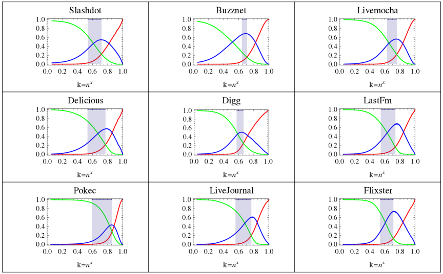
(a)
Network Nodes Edges Slashdot 51083 116573 Buzznet 101163 2763066 Livemocha 104103 2193083 Delicious 536408 1366136 Digg 771229 5907413 LastFm 1191812 4519340 Pokec 1632803 22301964 LiveJournal 2238731 12816184 Flixster 2523386 7918801 (b) (c)

Figure 3: (a) The elite influence shift diagrams (plotting the influence ratios $\mathcal{I}(\mathcal{E},\mathcal{E})/m$, $\mathcal{I}(\mathcal{P},\mathcal{P})/m$ and $\mathcal{I}(\mathcal{E},\mathcal{P})/m$) for the $k$-rich-clubs of nine networks. The X axis is on a logarithmic scale, where a point $x$ (in [0,1]) represents a $k$-rich club of size $k=n^{x}$. A point $y$ on the $Y$ axis indicates the fraction $\mathcal{I}(\cdot,\cdot)/m$, where $m$ is the total number of edges. The range of $x$ values between $x_{0}$ such that $k=\sqrt{m}=n^{x_{0}}$ and $x_{1}$, the symmetry point, such that $k=k_{sp}=n^{x_{1}}$ is highlighted. (b) Networks nodes and edges numbers. (c) Median results of the elite influence shift diagram for the $k$-rich-club elites for the $98$ networks examined, for increasing $k$.

5 Empirical Results

5.1 Symmetry Point and the Axioms

We investigated both the static properties of the network elites and their dynamics over time. In total we analyzed about $100$ social and complex networks. Their observed behavior (w.r.t. elite and periphery relationships) is surprisingly consistent. While it is clear that the issue of identifying the elite members of a given network is of paramount importance, with some recent developments [26, 32], this issue is not discussed in the present work. Instead, in order to conduct our experiments on given networks, we construct an approximation of the elite, $\mathcal{E}_{k}$, of size $k$. Once the $k$ members of the elite are selected, the rest of the vertices are considered as forming the periphery $\mathcal{P}_{k}$ (of size $n-k$), and the values of $I(\mathcal{E}_{k},\mathcal{E}_{k})$, $I(\mathcal{E}_{k},\mathcal{P}_{k})$ and $I(\mathcal{P}_{k},\mathcal{P}_{k})$ can be calculated directly. We use two known methods for approximating an elite $\mathcal{E}_{k}$ of size $k$. The first method is based on the notion of the $k$-rich-club, and we denote the size-$k$ elite it generates for a given network $G$ by $\mathcal{E}_{k}^{\mathrm{rich}}(G)$ (and omit $G$ and $\mathrm{rich}$ when they are clear from context). The second method relies on looking for a $c$-core in the network [12], and it is a bit more complex. The two methods produce different elites (albeit with some overlap). We present in the main text only the results for the $k$-rich-club elites, but similar results were obtained when we used the $c$-core method (see Appendix C for details on the results with the $c$-core method).

The $k$-rich-club [33] is perhaps the most intuitive and natural approximation for an elite of size $k$. To build it for a given network $G$, we sort the network vertices according to their degree, and choose the $k$ highest degree vertices as the members of $\mathcal{E}_{k}^{\mathrm{rich}}$ (breaking ties arbitrarily). Note that this method allows us to generate an elite for any desirable size $1\leq k\leq n$.

We present results from the $98$ networks we evaluated. (Detailed results are shown only for nine example networks, but the median values were calculated based on all the $98$ networks studied.) For each network we considered an elite selection method (i.e., $k$-rich-club or $c$-core) and then examined the influence and density of the elite and periphery and validated the axioms for different elite sizes and networks.

We first consider the elite influence shift diagrams which presents the changes in $\mathcal{I}(\mathcal{E}_{k},\mathcal{E}_{k})$, $\mathcal{I}(\mathcal{P}_{k},\mathcal{P}_{k})$ and $\mathcal{I}(\mathcal{E}_{k},\mathcal{P}_{k})$ as the elite (i.e., $\mathcal{E}^{k}_{\mathrm{rich}}(G)$) grows from its minimum size of $1$ to its maximum size of $n$. Figure 3 shows the elite influence shift diagrams of the $k$-rich-club for $9$ networks and the median results of the $k$-rich-club for all of the $98$ networks in our experiments. Note that the $X$-axis is logarithmic and presented as $k=n^{x}$ where $x$ goes from $0$ to $1$. The point $x=0.5$ therefore indicates a $\sqrt{n}$-rich-club. To normalize the $Y$-axis for different networks, each graph plots ${\mathcal{I}(\mathcal{E}_{k},\mathcal{E}_{k})}/{m}$, ${\mathcal{I}(\mathcal{P}_{k},\mathcal{P}_{k})}/{m}$, and ${\mathcal{I}(\mathcal{E}_{k},\mathcal{P}_{k})}/{m}$. Observe that the networks exhibit a similar pattern: the number of crossing edges between the elite and the periphery, $\mathcal{I}(\mathcal{E}_{k},\mathcal{P}_{k})$, grows with the elite size $k$ up to some maximum, and then starts decreasing. An interesting and less obvious pattern is that $\mathcal{I}(\mathcal{E}_{k},\mathcal{P}_{k})$ is larger than $\mathcal{I}(\mathcal{E}_{k},\mathcal{E}_{k})$ right from the beginning and remains larger until the maximum point. The relation between these numbers changes only after $\mathcal{I}(\mathcal{E}_{k},\mathcal{P}_{k})$ begins to decrease, while $\mathcal{I}(\mathcal{E}_{k},\mathcal{E}_{k})$ continues to grow.

As mentioned before, a particularly interesting point in these graphs is the symmetry point, namely, the elite size, denoted as $k_{sp}$, where the internal influence of the core and the internal influence of the periphery are equal, i.e., $\mathcal{I}(\mathcal{E}_{k_{sp}},\mathcal{E}_{k_{sp}})=\mathcal{I}(\mathcal{P}_{k_{sp}},\mathcal{P}_{k_{sp}})$. Recall that any elite that satisfies Axioms (A1), (A2) and (A3) must be near its symmetry point. An important observation (stated earlier in Observation 3.6) is that $\mathcal{I}(\mathcal{E}_{k},\mathcal{P}_{k})$ achieves it maximum at (or very close to) the symmetry point where $k=k_{sp}$.

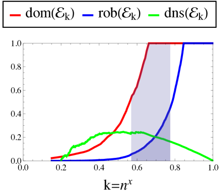
(a)
at $\sqrt{m}$ Min Max Median $\mathrm{dom}(\mathcal{E}_{k})$ 0.01 1+ 0.59 $\mathrm{rob}(\mathcal{E}_{k})$ 0.01 1+ 0.07 $\mathrm{dns}(\mathcal{E}_{k})$ 0 - 0.51 0.24 at symmetry point Min Max Median $\mathrm{dom}(\mathcal{E}_{k})$ 0.42 1+ 2.28 $\mathrm{rob}(\mathcal{E}_{k})$ 0.02 1+ 0.44 $\mathrm{dns}(\mathcal{E}_{k})$ 0 - 0.42 0.16 (b) (c)

Figure 4: (a) Observed dominance ratio, $\mathrm{dom}(\mathcal{E}_{k})$, observed robustness ratios, $\mathrm{rob}(\mathcal{E}_{k})$ and the observed density increase, $\mathrm{dns}(\mathcal{E}_{k})=\frac{\delta(\mathcal{E}_{k})-\delta}{\delta}$ for nine example networks. The x axis is logarithmic and marks the sizes of the $k$-rich-club elites with $k=n^{x}$. The highlighted area is $\mathcal{E}_{k}$’s of sizes between $k=\sqrt{m}$ and the symmetry point $k=k_{sp}$ (b) Median, Min and Max results for $98$ networks at $k=\sqrt{m}$ and $k=k_{sp}$. (c) Median results for $98$ networks.

One of the main contributions of this paper is the claim that elites in social networks are “small”, that is, of sub-linear size. We address this issue in detail shortly, but for now we note that in Figure 3, for both the example networks and the median of all networks, the symmetry point occurs mostly at elite sizes between $n^{0.6}$ and $n^{0.85}$, and its median value is at about $n^{0.77}$.

In all figures we highlight the range $[x_{0},x_{1}]$ of sizes for which it was shown that an elite can satisfy Axioms (A1) and (A2). More explicitly, this range starts at the lower bound on the elite size, i.e., the point $x_{0}$ such that $k=\sqrt{m}=n^{x_{0}}$, and ends at the symmetry point, i.e., the point $x_{1}$ such that $k=k_{sp}=n^{x_{1}}$. Note that since each network has different structure and different average degree, the values $x_{0}$ and $x_{1}$ are different for each network (hence in Figure 3 (c), the leftmost point $x_{0}$ of the highlighted range represents a median value).

We now turn to the claim that small elites, and in particular that elites near the symmetry point $k_{sp}$ satisfy Axioms (A1), (A2) and (A3), that is, they are dominant, robust and denser than the whole network. Recall that by Thm. 4.2, if an elite satisfies these three axioms, then its size must be sublinear. For a given network $G$ with elite $\mathcal{E}_{k}$ (of size $k$) and periphery $\mathcal{P}_{k}$, define the observed dominance ratio of $\mathcal{E}_{k}$ on $G$ as $\mathrm{dom}(\mathcal{E}_{k})=\mathcal{I}(\mathcal{E}_{k},\mathcal{P}_{k})/\mathcal{I}(\mathcal{P}_{k},\mathcal{P}_{k})$ and the observed robustness ratio of $\mathcal{E}$ on $G$ as $\mathrm{rob}(\mathcal{E}_{k})=\mathcal{I}(\mathcal{E}_{k},\mathcal{E}_{k})/\mathcal{I}(\mathcal{E}_{k},\mathcal{P}_{k})$. The observed density of the $\mathcal{E}_{k}$ is denoted as $\delta(\mathcal{E}_{k})$. Note that the density of the network is $\delta(\mathcal{E}_{n})$ and is denoted simply as $\delta$. We define the observed density increase as $\mathrm{dns}(\mathcal{E}_{k})=(\delta(\mathcal{E}_{k})-\delta)/\delta$, which indicates for each elite $\mathcal{E}_{k}$ the ratio by which it is denser than the whole graph.

Figure 4 (a) shows the values of the observed dominance and robustness ratios and the observed density increase, $\mathrm{dom}(\mathcal{E}_{k})$, $\mathrm{rob}(\mathcal{E}_{k})$ and $\mathrm{dns}(\mathcal{E}_{k})$ respectively, for the nine example networks $G$ with $k$-rich club elites of different sizes $k$. Figure 4 (c) shows the median of these values for all of the $98$ networks.

The X-axis for each graph is again on a logarithmic scale, where an $x$ value represents a $k$-rich-club of size $n^{x}$. We focus on values of $\mathrm{dom}(\mathcal{E}_{k})$ and $\mathrm{rob}(\mathcal{E}_{k})$ up to 1, and ignore higher values. As before, we highlight in each figure the range of $k$ for $k$-rich-club of sizes between $k=\sqrt{m}$ and the symmetry point $k=k_{sp}$.

Although it is not necessitated by the model or the axioms, it is clear from the figures that as the elite $\mathcal{E}_{k}$ grows in size, it attains more dominance over the rest of the network (the periphery, $\mathcal{P}_{k}$), namely, its observed dominance ratio increases, and its observed robustness ratio grows as well. We therefore focus on the highlighted area of interest. One can see that the social networks under study exhibit high values for both $\mathrm{dom}(\mathcal{E}_{k})$ and $\mathrm{rob}(\mathcal{E}_{k})$ at the highlighted area. Recall that by our previous analysis, elites that satisfy Axioms (A1) and (A2) are of size $k\geq\sqrt{m}$. Hence the smallest possible size for an elite is $k=\sqrt{m}$ and at that size, one might expect the elites to exhibit relatively small values of $\mathrm{dom}(\mathcal{E}_{k})$ and $\mathrm{rob}(\mathcal{E}_{k})$. Somewhat surprisingly, the calculated values are relatively high and are bounded away from zero. For example, At $k=\sqrt{m}$, the elite of ’Buzznet’ has observed dominance ratio $\mathrm{dom}(\mathcal{E}_{k})$ way beyond 1, and the elite of ’Digg’ has observed ratio of about 1, exhibiting high dominance over the rest of the network. ’Pocek’, which exhibits one of the lowest observed dominance ratios at $k=\sqrt{m}$, still has $\mathrm{dom}(\mathcal{E}_{k})$ of about $0.1$, which is also reasonably high. Figure 3(c) shows the median value of $\mathrm{dom}(\mathcal{E}_{k})$ of all $98$ networks. At $k=\sqrt{m}$, this median value is very high, about $0.6$, exhibiting very high dominance of elites of this size. The dominance of elites of size $k_{sp}$ at the symmetry point is even higher. All the example networks have observed dominance ratios $\mathrm{dom}(\mathcal{E}_{sp})>1$ so the median $\mathrm{dom}(\mathcal{E}_{sp})$ value is also greater than 1 at the symmetry point $k_{sp}$. These empirical results show that in real social networks, elites of size greater than $\sqrt{m}$ and smaller than the symmetry point exhibit high dominance and satisfy Axiom (A1). Similar results, albeit somewhat weaker, were obtained for $c$-core elites.

(a)

Network Duration (months) Epinions 31 Facebook 52 Flickr 7 Slashdot 33
(b)	(c)

Figure 5: (a) The fraction of the elite at the symmetry point, from the whole population, as the networks evolve over time. 4 examples. (b) Duration of the example networks (c) The median out of $8$ networks.

Observed robustness ratios exhibit a similar behavior to observed dominance ratios. For small elites of size $k=\sqrt{m}$, all the example networks have observed robustness ratios well bounded away from zero, and so is the median value for all $98$ networks. The lowest value of any of the example networks, observed for ’Flixter’, is $\mathrm{rob}(\mathcal{E}_{\sqrt{m}})=0.02$. The highest value, observed for ’Digg’, is $0.13$. The median observed robustness ratio at that point is about $0.1$. At the symmetry point $k_{sp}$ the observed ratios are higher. For example, ’Pokec’ has an observed robustness ratio of $\mathrm{rob}(\mathcal{E}_{sp})=0.65$, and the smallest value, observed for ’Flixter’, is $0.18$. The median value at that point is about $0.45$. Again, it follows that elites of size greater than $\sqrt{m}$ and smaller than the symmetry point in social networks have a high robustness. Similar results, in fact somewhat stronger, were obtained for the $c$-core elites. In general, elites produced by $c$-core exhibit lower dominance but higher robustness than those based on $k$-rich clubs.

Another interesting observation that can be deduced from Figures 4 is that in almost all the social networks that we tested, viewing elites of increasing size, we note that the elites attain dominance before attaining robustness.

Turning to density, the figures clearly reveal that the density of the elite, $\delta(\mathcal{E}_{k})$, is significantly higher than the density of the whole graph. The median results for $98$ networks exhibit that the elite at the symmetry point is about $20\%$ denser than the whole graph. The density at $k=\sqrt{m}$ is even higher. Interestingly, $\mathcal{E}_{k}$ seems to reach its maximum density around this point, when $k=\sqrt{m}$.

To conclude the discussion of Figure 4, we state that our empirical results provide strong evidence that it is a universal property that the $k$-rich-club elite, at its symmetry point, satisfies Axioms (A1), (A2) and (A4). From Theorem 4.2 we therefor conclude that $k_{sp}$, the elite size at the symmetry point, is a sublinear function of $n$.

5.2 The Scaling Law: Elite Size in growing networks

In the networks we examined so far, the sizes of the elites at the symmetry point (in both the $k$-rich-club and the $c$-core methods) appear to be sublinear, and specifically, between $n^{0.6}$ and $n^{0.85}$. Although this result was obtained for networks of different sizes, all of them were static, and therefore the data collection does not allow us to ascertain whether the size of the elite in the network’s symmetry point is indeed asymptotically sublinear.

To study this crucial question more carefully, we turned to data collected on dynamic networks, namely, networks for which information is available on their evolution over time. If the elite size at the symmetry point is indeed sublinear, then one should observe a decrease in the relative size of the elite (its fraction of the network size) as the network grows.

Figure 5 presents the data collected for dynamic networks. We evaluated $8$ networks for which information was available about the creation time of each edge. Using this information, we simulated the evolution of the network. As data on the appearance time of each network vertex was not available, we made the assumption that each vertex has joined the network at the same time when the first edge incident to it has appeared. We then divided the evolution time of the network into 20 time frames, each corresponding to a time period during which the network size increased by $5\%$ of the total (final) network size. For each time frame $t$, we calculated the elite $\mathcal{E}_{k}(t)$ and the symmetry point $k=k_{sp}(t)$ in the snapshot of the network at time $t$. Figure 5 shows the ratio $r=\lvert\mathcal{E}_{k_{sp}}(t)\rvert/n(t)=k_{sp}(t)/n(t)$ of the number of vertices in the elite at the symmetry point, where $k_{sp}(t)$ is the elite size at the symmetry point at time $t$ and $n(t)$ is the number of vertices in the entire network at time $t$. In each figure we added the trend of $\sqrt{m(t)}/n(t)$, where $m(t)$ is the number of edges in the network at time $t$. Clearly, unless the network is dense (i.e., with an order of $n(t)^{2}$ edges at time $t$), the ratio $\frac{\sqrt{m(t)}}{n(t)}$ converges to zero. Figure 5 (a) shows the results for four example networks out of the 8, and Figure  5 (b) shows the median result of all $8$ networks. These figures demonstrate that the elite size at the symmetry point is a relatively small fraction of the entire network (starting at a median of $10\%$ and ending at a median of $5\%$). Furthermore, it can be seen that as the network evolves and grows, the ratio $r$ decreases, following a pattern similar to the function $\sqrt{m(t)}$, implying that asymptotically indeed the elite size in the symmetry point has a sublinear size.

6 Related Work

As identifying the most influential vertices in a network is crucial to understanding its members’ behaviour, many studies considered a variety of notions related to the elite and core-periphery decompositions (see  [8] for a recent survey). Borgatti and Everett [4] measured the similarity between the adjaceny matrix of a graph and the block matrix ${1~{}1\choose 1~{}0}$. This captures the intuition that social networks have a dense, cohesive core and a sparse, disconnected periphery. Core/periphery networks revolve around a set of central vertices that are well-connected with each other as well as with the periphery. In addition to formalizing these intuitions, Borgatti and Everett devised algorithms for detecting core/periphery structures, along with statistical tests for verifying a-priori hypotheses [5]. Other efforts at identifying such structures and decomposing networks include a coefficient to measure if a network exhibits a clear-cut core-periphery dichotomy [16], a method to extract cores based on a modularity parameter [10] a centrality measure computed as a continuous value along a core-periphery spectrum [26], a coreness value attributed to each node, qualifying its position and role based on random walks [11], a detection method using spectral analysis and geodesic paths [9], and a decomposition method using statistical inference [32]. Mislove et al. [20] defined the core of a network to be any (minimal) set of vertices that satisfies two properties. First, the core must be essential for ensuring the connectivity of the network (i.e., removing it breaks the remainder of the vertices into many small, disconnected clusters). Second, the core must be strongly connected with a relatively small diameter. They observed that for such cores, the path lengths increase with the core size when progressively including vertices ordered inversely by their degree. The graphs studied in [20] have a densely connected core comprising of between 1% and 10% of the highest degree vertices, such that removing this core completely disconnects the graph. A recent article [31] argues that the core/periphery structure is simply the result of several overlapping communities and proposes a community detection method coping with overlap.

One of the first papers to focus on the fact that the highest degree vertices are well-connected  [33] coined the term rich-club coefficient for the density of the vertices of degree $k$ or more. Colizza et al. [7] refined this notion to account for the fact that higher degree vertices have a higher probability of sharing an edge than lower degree vertices, and suggested to use baseline networks to avoid a false identification of a rich-club. Xu et al. [30] shows that the rich-club connectivity has a strong influence on the assortativity and transitivity of a network. Weighted and hierarchical versions of the rich-club coefficient have been studied in [19, 22, 27, 34].

The nestedness of a network represents the likelihood of a vertex to be connected to the neighbors of higher degree vertices. Lee et al [17] defined a nestedness measure capturing the degree to which different groups in networks interact. Yet another perspective is offered in [15] where a network formation game and its equilibria are studied (benefits from connections exhibit decreasing returns and decay with network distance).

7 Discussion

In this article we address the forces responsible for the creation of elites in social networks. We provide axioms modeling the influence relationships between the elite and the periphery. We prove that at the power symmetry point, the size of the elite is sublinear in the size of the network. In particular that means that an elite is much smaller than a constant fraction of the network, evidence of which is often observed in the widening gap between the very rich and the rest of societies. To understand better what these axioms mean in practice, we studied a multitude of large real-world social networks. We approximated the elites by rich-clubs of various sizes. Our findings indicate that in these networks, rich-clubs near the symmetry point exhibit elite properties such as disproportionate dominance, robustness and density as stated by the axioms.

Our results do not only advance the theoretical understanding of the elite of social structures, but may also help to improve infrastructure and algorithms targeted at online social networks (e.g., [3]), organize institutions better or identify sources of power in social networks in general.

Appendix

Appendix A Extreme Elite Size

We have seen that a compact elite (satisfying axioms A1, A2, A3) has $\mathcal{I}(\mathcal{E},\mathcal{E})=\Omega(m)$ and $\mathcal{I}(\mathcal{E},\mathcal{P})=\Omega(m)$. A natural question is whether it is also guaranteed that $\mathcal{I}(\mathcal{P},\mathcal{P})=\Omega(m)$ (which may imply a stronger version of a symmetry point than the one defined earlier). We now demonstrate that unfortunately this is not the case. This is done by showing an example of a family of graphs with elites satisfying Axioms (A1), (A2), (A3), where $\mathcal{I}(\mathcal{E},\mathcal{E})=\Omega(m)$ and $\mathcal{I}(\mathcal{E},\mathcal{P})=\Omega(m)$ but $\mathcal{I}(\mathcal{P},\mathcal{P})=O(n)$.

We assume that the axioms are defined with constants $c_{r},c_{d}\leq 1$ and for simplicity we assume also that $c_{r}=1/b$ for constant integer $b$ (can easily be modified to a rational $c_{r}$, i.e., $c_{r}=a/b$ for constant integers $a,b$).

The construction of the graph uses a parameter $Z$ (to be thought of as roughly $n^{1/4}$), namely, the graph family contains one graph $G_{Z}$ for any integer $Z>0$.

The elite $\mathcal{E}$ consists of a complete network of $\varepsilon=|\mathcal{E}|=4Z^{3}-1$ vertices. the periphery $\mathcal{P}$ consists of $|\mathcal{P}|=2bZ\varepsilon=2bZ(4Z^{3}-1)$ vertices with no connections between them (except for a self-loop for each vertex). Hence altogether the graph $G_{Z}$ contains $n=8bZ^{4}+4Z^{3}-2bZ-1$ vertices.

Every vertex in $\mathcal{E}$ is connected to $2bZ^{3}$ vertices in $\mathcal{P}$, and every vertex in $\mathcal{P}$ is connected to $Z^{2}$ vertices in $\mathcal{E}$. Hence we have

$$\mathcal{I}(\mathcal{E},\mathcal{E}) = \varepsilon(\varepsilon+1)/2~{}=~{}2Z^{3}(4Z^{3}-1)$$

$$\mathcal{I}(\mathcal{E},\mathcal{P}) = Z^{2}|\mathcal{P}|~{}=~{}2bZ^{3}\varepsilon~{}=~{}2bZ^{3}(4Z^{3}-1)$$

$$\mathcal{I}(\mathcal{P},\mathcal{P}) = |\mathcal{P}|~{}=~{}2bZ(4Z^{3}-1)~{}.$$ (6)

Note that $n=\Theta(Z^{4})$ and $m=\Theta(Z^{6})=\Theta(n^{3/2})$, and indeed $\mathcal{I}(\mathcal{E},\mathcal{E}),\mathcal{I}(\mathcal{E},\mathcal{P})=\Omega(m)$ and $\mathcal{I}(\mathcal{P},\mathcal{P})=O(n)$.

We need to verify that this construction satisfies the three axioms. Axiom (A1) says that $\mathcal{I}(\mathcal{E},\mathcal{P})\geq c_{d}\cdot\mathcal{I}(\mathcal{P},\mathcal{P})$. This follows readily from Eq. (6) and the assumption that $c_{d}\leq 1$.

Axiom (A2) says that $\mathcal{I}(\mathcal{E},\mathcal{E})\geq\mathcal{I}(\mathcal{E},\mathcal{P})/b$. In fact, Eq. (6) establishes equality here.

To prove Axiom (A3), we need to show that every subset $\emptyset\subset\mathcal{E}^{\prime}\subset\mathcal{E}$ violates either axiom (A1) or (A2). Concretely, we show that it violates Axiom (A2), i.e., that

$$\mathcal{I}(\mathcal{E}^{\prime},\mathcal{E}^{\prime})~{}<~{}\mathcal{I}(\mathcal{E}^{\prime},\mathcal{P}^{\prime})/b.$$

Consider some $\emptyset\subset\mathcal{E}^{\prime}\subset\mathcal{E}$ and let $\mathcal{X}=\mathcal{E}\setminus\mathcal{E}^{\prime}$. Note that

$$\mathcal{I}(\mathcal{E}^{\prime},\mathcal{E}^{\prime}) = \mathcal{I}(\mathcal{E},\mathcal{E})-\mathcal{I}(\mathcal{X},\mathcal{E}^{\prime})-\mathcal{I}(\mathcal{X},\mathcal{X})$$

$$\mathcal{I}(\mathcal{E}^{\prime},\mathcal{P}^{\prime}) = \mathcal{I}(\mathcal{E},\mathcal{P})+\mathcal{I}(\mathcal{X},\mathcal{E}^{\prime})-\mathcal{I}(\mathcal{X},\mathcal{P})$$

hence we need to prove that

$$b\cdot(\mathcal{I}(\mathcal{E},\mathcal{E})-\mathcal{I}(\mathcal{X},\mathcal{E}^{\prime})-\mathcal{I}(\mathcal{X},\mathcal{X}))~{}<~{}\mathcal{I}(\mathcal{E},\mathcal{P})-\mathcal{I}(\mathcal{X},\mathcal{E}^{\prime})-\mathcal{I}(\mathcal{X},\mathcal{P})~{}.$$

Let $\chi=|\mathcal{X}|$ and $\varepsilon^{\prime}=|cE^{\prime}|=\varepsilon-\chi$. Then plugging the quantities of Eq. (6), it remains to prove that

$$b(2Z^{3}(4Z^{3}-1)-\chi(4Z^{3}-1-\chi)-\chi(\chi+1)/2)~{}<~{}2bZ^{3}(4Z^{3}-1)+\chi(4Z^{3}-1-\chi)-2bZ^{3}\chi~{}.$$

Simplifying, we get that the above indeed holds for every $\chi<\varepsilon$.

(a)	(b)

Figure 6: Extreme examples of elite-periphery partitions that satisfy our axioms and are close to the symmetry point. In both networks we assume each vertex has a self-loop edge that represents self-influence and is not drown for simplicity. Elite vertices are gray. (a) A “purely elitistic society” example with 41 vertices of which 6 are the elite. One can extend this example to a network of $n$ vertices where the number of edges is $m<2n$ edges. The elite then is of sub-linear size and consists of about $\sqrt{m}\approx\sqrt{n}$ vertices. But it is dense, namely, the elite contains about $m$ edges. The periphery also contains about $m$ edges so the partition is at a symmetry point. (b) A “purely egalitarian society” example of a grid network with 49 vertices from which 11 are the elite. This example can be extended to a network with $n$ vertices and $m<4n$ edges. It can be shown then that every dominant elite must be of size linear in $n$ (and $m$). It follows that both the elite and the periphery will have a linear number of edges and therefore the partition is close to the symmetry point. Most social networks observed in reality exhibit neither of these extreme behaviors.

Appendix B Symmetry in Random Networks

Let $\mathbf{d}=d_{1},d_{2},\dots,d_{n}$, where $1\leq d_{i}\leq n-1$ be a positive degree sequence. A random configuration graph $\mathcal{G}(n,\mathbf{d})$ is constructed in the following way over the set of vertices $[n]$. Let $W=[2m]$ be the set of configuration points where $m=\sum_{1}^{n}d_{i}/2$ is the number of edges. Define the ranges $W_{j}=[1+\sum_{1}^{j-1}d_{i}~{},~{}\sum_{1}^{j}d_{i}]$ for $j\in[n]$. Given a pairing $F$ (i.e., a partition of $W$ into $m$ pairs) we obtain a (multi) graph $G_{F}$ with vertex set $[n]$ and for each pair $(u,v)\in F$ we add an edge $(i,j)$ to $G_{F}$ where $u\in W_{i}$ and $v\in W_{j}$. Choosing $F$ uniformly from all possible pairings of $W$ we obtain a random (multi-)graph $\mathcal{G}(n,\mathbf{d})$.

For a given degree sequence $\mathbf{d}$, define its symmetry point $\kappa(\mathbf{d})$ as follows:

$$\kappa(\mathbf{d})=\arg\min_{j}\left\lvert\sum_{i=1}^{j}d_{i}-\sum_{i=j+1}^{n}d_{i}\right\rvert.$$

Given $\mathbf{d}$ and an index $1\leq i\leq n$, let $\mathcal{E}_{i}$ denote the core as the vertex set $[i]=\{1,\dots,i\}$ and the periphery $\mathcal{P}_{i}$ as the vertex set $\{i+1,\dots,n\}$.

Theorem B.1.

Let $\mathcal{G}(n,\mathbf{d})$ be a random configuration graph of given positive degree sequence $\mathbf{d}$ and let $\kappa$ be the symmetry point of $\mathbf{d}$ i.e., $\kappa(\mathbf{d})=\arg\min_{j}\left\lvert\sum_{i=1}^{j}d_{i}-\sum_{i=j+1}^{n}d_{i}\right\rvert$. Then,

1. $\mathbb{E}[\mathcal{I}(\mathcal{E}_{i},\mathcal{P}_{i})]\leq\mathbb{E}[\mathcal{I}(\mathcal{E}_{\kappa},\mathcal{P}_{\kappa})]$ for every $i$

2. $\mathbb{E}[\mathcal{I}(\mathcal{E}_{\kappa},\mathcal{P}_{\kappa})]\geq 4m/9$

3. $\mathbb{E}[\mathcal{I}(\mathcal{E}_{\kappa},\mathcal{E}_{\kappa})]\geq m/9$

4. $\mathbb{E}[\mathcal{I}(\mathcal{P}_{\kappa},\mathcal{P}_{\kappa})]\geq m/9$

Proof sketch. Let $D(k,l)=\sum_{i=k}^{l}d_{i}/2m$. Given a partition index $i$, the expected number of edges of each component is the following:

$$\mathbb{E}[\mathcal{I}(\mathcal{E}_{i},\mathcal{P}_{i})] = 2D(1,i)D(i+1,n)m,$$

$$\mathbb{E}[\mathcal{I}(\mathcal{E}_{i},\mathcal{E}_{i})] = D(1,i)^{2}m,$$

$$\mathbb{E}[\mathcal{I}(\mathcal{E}_{i},\mathcal{E}_{i})] = D(i+1,n)^{2}m.$$

Now, since $D(1,i)+D(i+1,n)=2m$, the maximum value of $D(1,i)D(i+1,n)$ is when $i=\arg\min_{j}\lvert D(1,i)-D(i+1,n)\rvert$ which is exactly $\kappa(\mathbf{d})$. What are lower bounds for the three influences? Note that $\lvert D(1,\kappa)-D(\kappa+1,n)\rvert$ will be maximized when $d_{\kappa}=n-1$ and $D(1,\kappa-1)=D(\kappa+1,n)$ so the worst case is when $D(1,\kappa-1)=D(\kappa+1,n)=n-1$ and $d_{\kappa}=n-1$, yielding the claimed result.

Appendix C $C$-Core Results

Figure 7: $c$-core elites: $\mathcal{I}(\mathcal{E},\mathcal{E})/m$, $\mathcal{I}(\mathcal{P},\mathcal{P})/m$ and $\mathcal{I}(\mathcal{E},\mathcal{P})/m$ for 9 networks for increasing $k_{c}$ and their medians for the $98$ networks in our measurements. A point $x$ on the $X$ axis shows a $c$-core of size $k_{c}=n^{x}$, for $x$ in the range [0,1]. The $Y$ axis gives the percentage of the measured value from the total number of edges. The range of $x$ values between $n^{x}=\sqrt{m}$ and the symmetry point is highlighted.

Section 5 described the results obtained when we examined the changes in $\mathcal{I}(\mathcal{E},\mathcal{E}),\mathcal{I}(\mathcal{P},\mathcal{P})$ and $\mathcal{I}(\mathcal{E},\mathcal{P})$ for various elite sizes when the elites were chosen using the $k$-rich-club method. In this section we consider the setting when the elites are chosen using the $c$-core mothod, and show the results obtained in this setting.

As in Figures 3, we show the changes in $\mathcal{I}(\mathcal{E},\mathcal{E})$, $\mathcal{I}(\mathcal{P},\mathcal{P})$ and $\mathcal{I}(\mathcal{E},\mathcal{P})$ as the elite grows from its minimum to its maximum possible size. In the $c$-core case, these sizes are determined by the network structure, and cannot be set by us. Specifically, the minimum size is the smallest possible $k_{c}>0$ and the maximum size is $k_{1}$.

Figure 7 shows our results for nine example networks and the median results for the $c$-cores of all $98$ networks included in our experiments. Each graph contains three plots. The first is for ${\mathcal{I}(\mathcal{E},\mathcal{E})}/{m}$, the second is for ${\mathcal{I}(\mathcal{P},\mathcal{P})}/{m}$ and the third is for ${\mathcal{I}(\mathcal{E},\mathcal{P})}/{m}$. The X-axis for each graph is on a logarithmic scale, where an $x$ value represents a $c$-core of size $k_{c}=n^{x}$. Although the results in the setting of $c$-core elites are not as consistent and smooth for all networks as in the setting of $k$-rich-club elites, one can observe that the results here are similar to those obtained in the $k$-rich-club setting. Here, too, most of the networks exhibit similar patterns: as the elite size grows, $\mathcal{I}(\mathcal{E},\mathcal{E})$ grows as well and $\mathcal{I}(\mathcal{P},\mathcal{P})$ decreases, while the number of crossing edges $\mathcal{I}(\mathcal{E},\mathcal{P})$ grows with the elite size up to some maximum and then starts decreasing. Here too, $\mathcal{I}(\mathcal{E},\mathcal{P})$ is larger than $\mathcal{I}(\mathcal{E},\mathcal{E})$ (almost) right from the beginning and remains larger until the maximum point, and this relation changes only after $\mathcal{I}(\mathcal{E},\mathcal{P})$ begins to decrease (while $\mathcal{I}(\mathcal{E},\mathcal{E})$ continues to grow).

Figures 7 also show that in the setting of $c$-core elites, just as with $k$-rich-club elites (as mentioned in Section 3), $\mathcal{I}(\mathcal{E},\mathcal{P})$ attains its maximum at (or very close to) the symmetry point.

Figure 8: Dominance and robustness constants for the nine example networks and their median for the $98$ networks. The x axis is logarithmic and represents the sizes of $c$-cores with $k=n^{x}$. The higlighted area of $x$ values corresponds to sizes between $k_{c}=\sqrt{m}$ and the symmetry point.

Section 5 presented also the values of the dominance and robustness constants, $\rho_{d}$ and $\rho_{r}$ respectively, for various elite sizes in the setting of $k$-rich-club elites. Here, we present the corresponding results for $c$-core elites.

As in Figure 4 we show the changes in $\rho_{d}$ and $\rho_{r}$ as the elite grows from its minimum to its maximum possible size. Figure 8 shows results for our nine example networks and the median results for the $c$-core elites of all the $98$ networks included in our experiments. The X-axis for each graph is, again, on a logarithmic scale, where an $x$ value represents a $c$-core of size $k_{c}=n^{x}$. There are two plots in each graph, one for the dominance constant $\rho_{d}$ and the other for the robustness constant $\rho_{r}$. We focus on values of $\rho_{d}$ and $\rho_{r}$ up to 1, and ignore higher values. As before, we highlight in each figure the $c$-cores of sizes in the range $\sqrt{m}\leq k_{c}\leq SP$.

Clearly, elites chosen by the $c$-core method are different from same size elites chosen by the $k$-rich-club method. Indeed, the results presented for the $c$-core setting are not as consistent as in the $k$-rich-club setting. Nevertheless, our results show that the same basic characteristics, namely, high dominance and robustness in elites of sizes in the range of $\sqrt{m}\leq k_{c}\leq SP$, hold also for $c$-core elites. It is worth mentioning that in the setting of $c$-core elites, it does not hold for all networks that dominance is achieved before robustness.

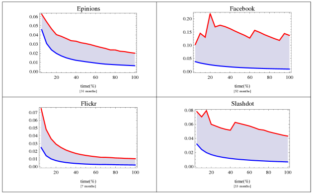
Figure 9: The fraction of the elite at the symmetry point, from the whole population, as the networks evolve over time. 4 examples and the median out of $8$ networks. Elites are chosen by $c$-core method.

Finally, turning to dynamic data, in Fig. 9 we repeated in the $c$-core setting the analysis of Fig. 5 from Section 5 for the $k$-rich-club setting. Specifically, we looked at the percentage of the number of vertices in the elite, $r~{}=~{}\frac{\lvert\mathcal{E}_{sp}\rvert}{n}$, for elite sizes $\lvert\mathcal{E}_{sp}\rvert$ at the symmetry point. We used the same assumptions made in Section 5 about the time information and followed the same procedure as described therein. Fig. 9 depicts the ratio $r$ as it evolves in time. Figure 9 shows the results for four example networks (this is a different set from the nine networks studied above, and the median result of all $8$ networks for which evolutionary data was available to us. Once again, the results in the setting of $c$-core elites are not as smooth as in the setting of $k$-rich-club elites. Nevertheless, here too the figures demonstrate that the elite size at the symmetry point is a relatively small portion of the entire network (starting at median of $9\%$ and ending at median of $6\%$). Furthermore, elites chosen by the $c$-core method exhibit similar behavior of evolution and growth as the $k$-rich-club setting. Here too the ratio $r$ decrease, implying that asymptotically, the elite size at the symmetry point is indeed sub-linear.

Appendix D Datasets

Data	Repository	$n$	$m$	Average Degree	Max Degree	Undirected Directed	Duration (months)	Description
Academia  BGU-Academia bguAcademia1bguAcademia2	BGU	200169	1022441	5.1	10693	D		Platform for academics to share research papers.
Blog  ASU-BlogZafarani+Liu:2009	ASU	88784	2093195	23.6	9444	U		Social blog directory which manages bloggers their blog
Blog2  ASU-Blog2Zafarani+Liu:2009	ASU	97884	1668647	17.0	27849	U		Social blog directory which manages bloggers their blog
Blog3  ASU-Blog3Zafarani+Liu:2009	ASU	10312	333983	32.4	3992	U		Social blog directory which manages bloggers their blog
Buzznet  ASU-BuzznetZafarani+Liu:2009	ASU	101163	2763066	27.3	64289	U		Photo, journal, and video-sharing social media network
Delicious  ASU-DeliciousZafarani+Liu:2009	ASU	536408	1366136	2.5	3216	U		Social bookmarking web service for storing sharing and discovering web bookmarks
Digg  ASU-DiggZafarani+Liu:2009	ASU	771229	5907413	7.7	17643	U		Social news website
Douban  ASU-DoubanZafarani+Liu:2009	ASU	154908	327162	2.1	287	U		Chinese website providing user review and recommendation services for movies books and music
Flickr  ASU-FlickrZafarani+Liu:2009	ASU	80513	5899882	73.3	5706	U		An image hosting and video hosting website web services suite and online community
Flixster  ASU-FlixsterZafarani+Liu:2009	ASU	2523386	7918801	3.1	1474	U		Social movie site allowing users to share movie ratings discover new movies and meet others with similar movie taste
Foursquare  ASU-FoursquareZafarani+Liu:2009	ASU	639014	3214986	5.0	106218	U		Location-based social networking website software for mobile devices. This service is available to users with GPS enabled mobile devices such as iPhones and Blackberries
Friendster  ASU-FriendsterZafarani+Liu:2009	ASU	5689498	14067887	2.5	4423	U		Social networking website.The service allows users to contact other members maintain those contacts and share online content and media with those contacts.
Hyves  ASU-HyvesZafarani+Liu:2009	ASU	1402673	2777419	2.0	31883	U		The most popular social networking site in the Netherlands with mainly Dutch visitors and members and competes in this country with sites such as Facebook and MySpace.
LastFm  ASU-LastFmZafarani+Liu:2009	ASU	1191812	4519340	3.8	5150	U		Music website founded in the United Kingdom in 2002. It has claimed over 40 million active users based in more than 190 countries.
LiveJournal  ASU-LiveJournalZafarani+Liu:2009	ASU	2238731	12816184	5.7	5873	U		Virtual community where Internet users can keep a blog journal or diary
Livemocha  ASU-LivemochaZafarani+Liu:2009	ASU	104103	2193083	21.1	2980	U		The world’s largest online language learning community offering free and paid online language courses in 35 languages to more than 6 million members from over 200 countries around the world.
Twitter  ASU-TwitterZafarani+Liu:2009	ASU	11316811	63555749	5.6	564795	D		Social news website. It can be viewed as a hybrid of email instant messaging and sms messaging all rolled into one neat and simple package. It’s a new and easy way to discover the latest news related to subjects you care about.
YouTube  ASU-YouTubeZafarani+Liu:2009	ASU	13723	76765	5.6	534	U		Video-sharing website on which users can upload share and view videos
YouTube-2  ASU-YouTube-2Zafarani+Liu:2009	ASU	13242	1940806	146.6	3068	U		Video-sharing website on which users can upload share and view videos
YouTube-3  ASU-YouTube-3Zafarani+Liu:2009	ASU	11765	5574249	473.8	6745	U		Video-sharing website on which users can upload share and view videos
YouTube-4  ASU-YouTube-4Zafarani+Liu:2009	ASU	10455	2239440	214.2	5958	U		Video-sharing website on which users can upload share and view videos
YouTube-5  ASU-YouTube-5Zafarani+Liu:2009	ASU	13160	3797635	288.6	5759	U		Video-sharing website on which users can upload share and view videos
AnyBeat  BGU-AnyBeatbguAnyBeat	BGU	12645	49132	3.9	4800	D		Online community. A public gathering place where you can interact with people from around your neighborhood or across the world
GooglePlus  BGU-GooglePlusbguAcademia2	BGU	211186	1141650	5.4	1790	D		Google+ is a social networking service and website offered by Google
TheMarkerCafe  BGU-TheMarkerCafebguAcademia1bguAcademia2	BGU	69413	1644843	23.7	8930	U		Israeli online social network site that allows its member to connect and interact
arXivHep-thKDDCup  Konect-arXivHep-thKDDCup-ReferenceKonectb619	Konect	27769	352285	12.7	2468	D		Citation network from arXiv’s section on high energy physics theory (hep-th) as used in the KDD cup 2003.
BaiduInternal  Konect-BaiduInternal-ReferenceKonectkonect:zhishi	Konect	2140198	17014946	8.0	97848	D		Hyperlinks between the articles of the Chinese online encyclopedia Baidu.
BaiduRelated  Konect-BaiduRelated-ReferenceKonectkonect:zhishi	Konect	415624	2374044	5.7	127066	D		”Related to” links between articles of the Chinese online encyclopedia Baidu.
Catster  Konect-Catster-SocialKonect	Konect	149684	5448196	36.4	80634	U		This Network contains friendships between users of the website catster.com.
CatsterDogster  Konect-CatsterDogster-SocialKonect	Konect	623748	15695166	25.2	80636	U		Familylinks between cats and cats cats and dogs as well as dogs and dogs from the social websites catster.com and dogster.com. Also included are cat-cat and dog-dog friendships.
CiteSeer  Konect-CiteSeer-ReferenceKonectb524	Konect	384054	1736172	4.5	1739	D		Citation network extracted from the CiteSeer digital library.
CoraCitation  Konect-CoraCitation-ReferenceKonectkonect:dependency4	Konect	23166	89157	3.8	377	D		Cora citation network.
DBLP  Konect-DBLP-ContactKonectkonect:DBLP	Konect	1103412	4225686	3.8	1189	U	913	Collaboration graph of authors of scientific papers from DBLP computer science bibliography
Digg  Konect-Digg-CommunicationKonectkonect:choudhury09	Konect	30360	85155	2.8	283	D		Reply network of the social news website Digg
Dogster  Konect-Dogster-SocialKonect	Konect	426816	8543548	20.0	46503	U		This Network contains friendships between users of the website dogster.com.
Epinions  Konect-Epinions-SocialKonectkonect:massa05	Konect	131580	711210	5.4	3558	D	31	Trust and distrust network of Epinions, an online product rating site
Facebook  Konect-Facebook-CommunicationKonectviswanath09	Konect	45813	183412	4.0	223	D	52	Directed network of a small subset of posts to other user’s wall on Facebook
Facebook-WOSN  Konect-Facebook-WOSN–SocialKonectviswanath09	Konect	63731	817090	12.8	1098	U	29	Friendship data of facebook users
Flickr  Konect-Flickr-SocialKonectb494	Konect	2302925	22838276	9.9	27937	D	7	Social network of users and their friendship connections
FlickrLinks  Konect-FlickrLinks-SocialKonectkonect:mislove	Konect	1715255	15555041	9.1	27236	U		Social network of Flickr users and their connections.
HudongInternal  Konect-HudongInternal-ReferenceKonectkonect:zhishi	Konect	1974655	14428382	7.3	61440	D		Hyperlinks between articles of the Chinese online encyclopedia Hudong.
HudongRelated  Konect-HudongRelated-ReferenceKonectkonect:zhishi	Konect	2452673	18691099	7.6	204282	D		”Related to” links between articles of the Chinese online encyclopedia Hudong.
LibimsetiCZ  Konect-LibimsetiCZ-SocialKonectkonect:kunegis2012konect:brozovsky07	Konect	220970	17233144	78.0	33389	D		Czech dating site. This is the network of ratings given by users to other users.
PrettyGoodPrivacy  Konect-PrettyGoodPrivacy-ContactKonectkonect:boguna	Konect	10680	24316	2.3	205	U		Interaction network of users of the Pretty Good Privacy (PGP) algorithm.
Slashdot  Konect-Slashdot-CommunicationKonectkonect:slashdot-threads	Konect	51083	116573	2.3	2915	D	33	Reply network of technology website
SlashdotZoo  Konect-SlashdotZoo-SocialKonectkunegis:slashdot-zoo	Konect	79120	467869	5.9	2537	D		Signed social network of users of the technology news site Slashdot connected by directed ”friend” and ”foe” relations.
TRECWT10g  Konect-TRECWT10g-ReferenceKonectb397	Konect	1601787	6679248	4.2	25609	D		Web Research Collections (TREC Web, Terabyte and Blog Tracks)
TwitterICWSM  Konect-TwitterICWSM-SocialKonectkonect:choudhury10	Konect	465017	833541	1.8	677	D		Who follows whom on Twitter.
USpatents  Konect-USpatents-ReferenceKonectb376	Konect	3774768	16518947	4.4	793	D		Citation network of patents registered with the United States Patent and Trademark Office.
WikipediaChinese  Konect-WikipediaChinese-ReferenceKonectkonect:zhishi	Konect	1930270	8956902	4.6	29005	D		Network of hyperlinks between the articles of Wikipedia in Chinese.
WikipediaEnglish  Konect-WikipediaEnglish-ReferenceKonectkonect:mislove2	Konect	1870709	36532531	19.5	226073	D	75	Hyperlink network of the English Wikipedia with edge arrival times.
WikipediaLinksDE  Konect-WikipediaLinksDE-ReferenceKonect	Konect	3783012	68714064	18.2	437732	D		Wikilinks inside the German Wikipedia.
WikipediaLinksFR  Konect-WikipediaLinksFR-ReferenceKonect	Konect	4905934	104591689	21.3	1274642	D		Wikilinks inside the French Wikipedia.
WikipediaLinksIT  Konect-WikipediaLinksIT-ReferenceKonect	Konect	2790019	86754664	31.1	825147	D		Wikilinks inside the Italian Wikipedia.
WikipediaLinksJA  Konect-WikipediaLinksJA-ReferenceKonect	Konect	2140579	58200970	27.2	390239	D		Wikilinks inside the Japanese Wikipedia.
WikipediaLinksPL  Konect-WikipediaLinksPL-ReferenceKonect	Konect	1646203	41216900	25.0	215361	D		Wikilinks inside the Polish Wikipedia.
WikipediaLinksPT  Konect-WikipediaLinksPT-ReferenceKonect	Konect	2804569	51539953	18.4	628617	D		Wikilinks inside the Portuguese Wikipedia.
WikipediaLinksRU  Konect-WikipediaLinksRU-ReferenceKonect	Konect	2819989	64066427	22.7	587438	D		Wikilinks inside the Russian Wikipedia.
YouTube  Konect-YouTube-SocialKonectkonect:mislove2	Konect	3223589	9376594	2.9	91751	U	7	Video-sharing website on which users can upload share and view videos. Social network of users and their friendship connections
Amazon  SNAP-AmazonDBLP:journals/corr/abs-1205-6233	SNAP	334863	925872	2.8	549	U		Based on ’Customers Who Bought This Item Also Bought’ feature of the Amazon website. If a product i is frequently co-purchased with product j the graph contains an undirected edge from i to j.
amazon0302  SNAP-amazon0302leskovec2007graph	SNAP	262111	899792	3.4	420	D		Amazon product co-purchasing network from March 2 2003
amazon0312  SNAP-amazon0312leskovec2007graph	SNAP	400727	2349869	5.9	2747	D		Amazon product co-purchasing network from March 12 2003
as-Caida  SNAP-as-Caidaleskovec2005graphs	SNAP	26475	53381	2.0	2628	D		The CAIDA AS Relationships Datasets, from January 2004 to November 2007
as-Skitter  SNAP-as-Skitterleskovec2005graphs	SNAP	1696415	11095298	6.5	35455	U		Internet topology graph, from traceroutes run daily in 2005
ca-AstroPh  SNAP-ca-AstroPhLeskovec:2007:GED:1217299.1217301	SNAP	18771	198050	10.6	504	U		Arxiv ASTRO-PH (Astro Physics) collaboration network
ca-CondMat  SNAP-ca-CondMatLeskovec:2007:GED:1217299.1217301	SNAP	23133	93439	4.0	279	U		Arxiv COND-MAT (Condense Matter Physics) collaboration network
ca-HepPh  SNAP-ca-HepPhLeskovec:2007:GED:1217299.1217301	SNAP	12006	118489	9.9	491	U		Arxiv HEP-PH (High Energy Physics - Phenomenology) collaboration network
cit-Patents  SNAP-cit-PatentsLeskovec:2005:GOT:1081870.1081893	SNAP	3774768	16518947	4.4	793	D		Citations made by patents granted between 1975 and 1999
cit-HepPh  SNAP-cit-HepPhLeskovec:2005:GOT:1081870.1081893gehrke03kddcup	SNAP	34546	420877	12.2	846	D		Arxiv HEP-PH (high energy physics phenomenology) citation graph. If a paper i cites paper j the graph contains a directed edge from i to j
cit-HepTh  SNAP-cit-HepThLeskovec:2005:GOT:1081870.1081893gehrke03kddcup	SNAP	27769	352285	12.7	2468	D		Arxiv HEP-TH (high energy physics theory) citation graph. If a paper i cites paper j the graph contains a directed edge from i to j
DBLP  SNAP-DBLPDBLP:journals/corr/abs-1205-6233	SNAP	317080	1049866	3.3	343	U		Co-authorship network from DBLP computer science bibliography, where two authors are connected if they publish at least one paper together.
ego-Gplus  SNAP-ego-Gplusmcauley2012learning	SNAP	107614	12238285	113.7	20127	D		Social circles from Google+
ego-Twitter  SNAP-ego-Twittermcauley2012learning	SNAP	81306	1342296	16.5	3383	D		Social circles from Twitter
email-Enron  SNAP-email-Enronleskovec2009communityklimt2004introducing	SNAP	36692	183831	5.0	1383	U		Email communication network from Enron
email-EuAll  SNAP-email-EuAllleskovec2007graph	SNAP	265009	364481	1.4	7636	D		Email network from a EU research institution
epinions  SNAP-epinionsrichardson2003trust	SNAP	75879	405740	5.3	3044	D		General consumer review site. An online social network of Who-trust-whom.
flickr  SNAP-flickrmcauley2012image	SNAP	105943	2316952	21.9	5425	U		Images sharing common metadata on Flickr
higgs-twitter-friendship  SNAP-higgs-twitter-friendshipDMM2013	SNAP	456631	12508442	27.4	51386	D		Spreading processes of the announcement of the discovery of a new particle with the features of the Higgs boson on 4th July 2012.
higgs-twitter-mention  SNAP-higgs-twitter-mentionDMM2013	SNAP	302523	436816	1.4	22790	D		Spreading processes of the announcement of the discovery of a new particle with the features of the Higgs boson on 4th July 2012.
higgs-twitter-retweet  SNAP-higgs-twitter-retweetDMM2013	SNAP	425008	732790	1.7	31556	D		Spreading processes of the announcement of the discovery of a new particle with the features of the Higgs boson on 4th July 2012.
LiveJournal  SNAP-LiveJournalbackstrom-group-2006DBLP:journals/corr/abs-0810-1355	SNAP	4846609	42851237	8.8	20333	D		Virtual community where Internet users can keep a blog journal or diary
LiveJournalCom  SNAP-LiveJournalComDBLP:journals/corr/abs-1205-6233	SNAP	3997962	34681189	8.7	14815	U		Virtual community where Internet users can keep a blog journal or diary
loc-brightkite  SNAP-loc-brightkitecho2011friendship	SNAP	58228	214078	3.7	1134	U		Location-based social networking service provider where users shared their locations by checking-in.
loc-gowalla  SNAP-loc-gowallacho2011friendship	SNAP	196591	950327	4.8	14730	U		Location-based social networking website where users share their locations by checking-in.
Oregon-1-1  SNAP-Oregon-1-1leskovec2005graphs	SNAP	10670	22002	2.1	2312	U		AS peering information inferred from Oregon route-views between March 31 and May 26 2001
Oregon-2-1  SNAP-Oregon-2-1leskovec2005graphs	SNAP	10900	31180	2.9	2343	U		AS peering information inferred from Oregon route-views between March 31 and May 26 2001
p2p-Gnutella31  SNAP-p2p-Gnutella31leskovec2007graphripeanu2002mapping	SNAP	62586	147892	2.4	95	D		Gnutella peer to peer network from August 31 2002
Pokec  SNAP-Pokectakac2012data	SNAP	1632803	22301964	13.7	14854	D		Pokec is the most popular on-line social network in Slovakia.
roadNet-CA  SNAP-roadNet-CAleskovec2009community	SNAP	1965206	2766607	1.4	12	U		Road network of California
roadNet-PA  SNAP-roadNet-PAleskovec2009community	SNAP	1088092	1541898	1.4	9	U		Road network of Pennsylvania
roadNet-TX  SNAP-roadNet-TXleskovec2009community	SNAP	1379917	1921660	1.4	12	U		Road network of Texas
slashdot1  SNAP-slashdot1DBLP:journals/corr/abs-0810-1355	SNAP	77360	469180	6.1	2539	D		Technology-related news website. Friend/foe network. Obtained in November 2008.
web-BerStan  SNAP-web-BerStanDBLP:journals/corr/abs-0810-1355	SNAP	685230	6649470	9.7	84230	D		Nodes represent pages from berkely.edu and stanford.edu domains and directed edges represent hyperlinks between them. The data was collected in 2002.
web-Google  SNAP-web-GoogleDBLP:journals/corr/abs-0810-1355	SNAP	875713	4322051	4.9	6332	D		Nodes represent web pages and directed edges represent hyperlinks between them. The data was released in 2002 by Google as a part of Google Programming Contest
web-NotreDame  SNAP-web-NotreDamealbert1999internet	SNAP	325729	1090108	3.3	10721	D		Nodes represent pages from University of Notre Dame (domain nd.edu) and directed edges represent hyperlinks between them. The data was collected in 1999 by Albert Jeong and Barabasi.
web-Stanford  SNAP-web-StanfordDBLP:journals/corr/abs-0810-1355	SNAP	281903	1992636	7.1	38625	D		Nodes represent pages from Stanford University (stanford.edu) and directed edges represent hyperlinks between them.
wiki-talk  SNAP-wiki-talkleskovec2010signedleskovec2010predicting	SNAP	2394385	4659565	1.9	100029	D		Wikipedia’s registered users talk pages. A directed edge from node i to node j represents that user i at least once edited a talk page of user j.
YouTube  SNAP-YouTubeDBLP:journals/corr/abs-1205-6233	SNAP	1134890	2987624	2.6	28754	U		Video-sharing website on which users can upload share and view videos. Social network of users and their friendship connections

Table 1: List of All Tested Networks

Appendix E Dominance and robustness

	$\rho_{d}$		$\rho_{r}$
Data	$\sqrt{m}$	SP	$\sqrt{m}$	SP
Blog	2.64	3.54	0.19	0.28
Blog2	6.52	6.16	0.17	0.16
Blog3	3.23	3.58	0.25	0.28
Buzznet	2.47	4.30	0.10	0.23
Delicious	0.35	2.62	0.04	0.38
Digg	0.88	1.96	0.13	0.51
Douban	0.18	4.50	0.07	0.22
Flickr	0.72	1.38	0.31	0.73
Flixster	0.40	5.50	0.02	0.18
Foursquare	1.20	2.35	0.04	0.43
Friendster	0.54	13.79	0.01	0.07
Hyves	0.32	6.28	0.02	0.16
LastFm	0.44	4.06	0.03	0.25
LiveJournal	0.33	3.07	0.02	0.33
Livemocha	0.81	2.57	0.10	0.39
Twitter	3.15	8.40	0.04	0.12
YouTube	0.51	1.89	0.07	0.53
YouTube 2	1.40	1.72	0.43	0.58
YouTube 3	2.66	2.16	0.60	0.46
YouTube 4	1.49	1.52	0.62	0.66
YouTube 5	3.21	2.39	0.60	0.42
Academia	0.27	1.65	0.06	0.61
AnyBeat	2.17	3.11	0.19	0.32
GooglePlus	0.38	0.91	0.19	1.10
TheMarkerCafe	1.46	2.60	0.18	0.38
arXivHep-thKDDCup Reference	0.45	1.34	0.10	0.75
BaiduInternal Reference	0.54	2.63	0.03	0.38
BaiduRelated Reference	1.02	2.86	0.19	0.35
CatsterDogster Social	1.08	2.32	0.17	0.43
Catster Social	3.57	4.12	0.20	0.24
CiteSeer Reference	0.19	2.12	0.01	0.47
CoraCitation Reference	0.30	1.83	0.05	0.55
DBLP Contact	0.09	1.36	0.07	0.73
Digg Communication	0.34	1.99	0.09	0.50
Dogster Social	1.32	2.93	0.11	0.34
Epinions Social	0.88	1.85	0.18	0.54
Facebook Communication	0.18	1.22	0.10	0.82
Facebook WOSN Social	0.25	1.13	0.16	0.89
FlickrLinks Social	0.62	1.19	0.22	0.84
Flickr Social	0.60	1.22	0.20	0.82
HudongInternal Reference	0.81	3.89	0.01	0.26
HudongRelated Reference	0.55	9.61	0.01	0.10
LibimsetiCZ Social	1.15	3.18	0.08	0.31
PrettyGoodPrivacy Contact	0.26	0.85	0.36	1.18
SlashdotZoo Social	0.63	2.14	0.11	0.47
Slashdot Communication	0.55	2.40	0.09	0.42
TRECWT10g Reference	0.54	3.46	0.01	0.29
TwitterICWSM Social	1.17	57.05	0.01	0.02
USpatents Reference	0.03	1.40	0.04	0.71
WikipediaChinese Reference	0.54	2.54	0.06	0.39
WikipediaEnglish Reference	0.73	3.07	0.03	0.33
WikipediaLinksDE Reference	0.58	2.62	0.01	0.38
WikipediaLinksFR Reference	1.00	3.16	0.01	0.32
WikipediaLinksIT Reference	0.99	2.62	0.03	0.38
WikipediaLinksJA Reference	0.72	2.57	0.03	0.39
WikipediaLinksPL Reference	0.63	1.97	0.08	0.51
WikipediaLinksPT Reference	1.17	3.19	0.05	0.31
WikipediaLinksRU Reference	0.76	2.24	0.02	0.45
YouTube Social	0.77	2.16	0.03	0.46
Amazon	0.07	3.05	0.01	0.33
amazon0302	0.07	2.14	0.02	0.47
amazon0312	0.11	2.42	0.01	0.41
as-Caida	2.18	6.03	0.07	0.17
as-Skitter	0.65	2.82	0.03	0.35
ca-AstroPh	0.35	1.17	0.20	0.85
ca-CondMat	0.23	1.41	0.11	0.71
ca-HepPh	0.34	0.42	1.49	2.41
cit-HepPh	0.31	1.62	0.07	0.62
cit-HepTh	0.45	1.34	0.10	0.75
cit Patents	0.03	1.40	0.04	0.71
DBLP	0.08	1.43	0.20	0.70
ego-Gplus	1.31	1.83	0.30	0.55
ego-Twitter	0.42	1.76	0.11	0.57
email-Enron	0.90	1.76	0.16	0.57
email-EuAll	4.13	10.07	0.05	0.10
epinions	0.76	1.65	0.20	0.61
flickr	0.35	0.93	0.55	1.08
higgs-twitter-friendship	1.06	3.45	0.02	0.29
higgs-twitter-mention	1.36	5.63	0.01	0.18
higgs-twitter-retweet	1.63	6.83	0.01	0.15
LiveJournal	0.12	1.04	0.10	0.96
LiveJournalCom	0.10	1.08	0.11	0.93
loc-brightkite	0.39	1.39	0.18	0.72
loc-gowalla	0.38	1.23	0.13	0.81
Oregon-1-1	2.81	5.86	0.08	0.17
Oregon-2-1	1.97	3.10	0.18	0.32
p2p-Gnutella31	0.09	2.27	0.02	0.44
Pokec	0.08	1.53	0.04	0.65
roadNet-CA	0.01	0.87	0.01	1.15
roadNet-PA	0.01	0.97	0.01	1.03
roadNet-TX	0.01	0.87	0.01	1.16
slashdot1	0.63	2.14	0.11	0.47
web-BerStan	1.12	2.30	0.01	0.43
web-Google	0.26	2.31	0.01	0.43
web-NotreDame	0.42	1.66	0.12	0.60
web-Stanford	1.14	2.56	0.01	0.39
wiki-talk	3.06	9.48	0.05	0.11
YouTube	0.57	1.96	0.04	0.51
Median	0.59	2.28	0.07	0.44
Average	0.95	3.41	0.13	0.51
STD	1.06	5.90	0.19	0.33
Min	0.01	0.42	0.01	0.02

Table 2: Domination and robustness values at the symmetry point and $\sqrt{m}$ of all Networks.

acm social

References

- [1] Alberich, R., Miro-Julia, J., and Rosselló, F. Marvel universe looks almost like a real social network. arXiv preprint cond-mat/0202174 (2002).
- [2] Albert, R., and Barabási, A. Statistical mechanics of complex networks. Reviews of modern physics 74, 1 (2002), 47–97.
- [3] Avin, C., Borokhovich, M., Lotker, Z., and Peleg, D. Distributed computing on core-periphery networks: Axiom-based design. In Automata, Languages, and Programming - 41st International Colloquium, ICALP 2014, Proceedings, Part II (2014), pp. 399–410.
- [4] Borgatti, S., and Everett, M. Models of core/periphery structures. Social networks 21, 4 (2000), 375–395.
- [5] Borgatti, S., Everett, M., and Freeman, L. Ucinet: Software for social network analysis. Harvard Analytic Technologies 2006 (2002).
- [6] Borgatti S.P., E. M. . J. J. Analyzing Social Networks. London: Sage Publications, 2013.
- [7] Colizza, V., Flammini, A., Serrano, M., and Vespignani, A. Detecting rich-club ordering in complex networks. Nature Physics 2, 2 (2006), 110–115.
- [8] Csermely, P., London, A., Wu, L.-Y., and Uzzi, B. Structure and dynamics of core/periphery networks. Journal of Complex Networks 1, 2 (2013), 93–123.
- [9] Cucuringu, M., Rombach, M. P., Lee, S. H., and Porter, M. A. Detection of core-periphery structure in networks using spectral methods and geodesic paths. arXiv preprint arXiv:1410.6572 (2014).
- [10] Da Silva, M. R., Ma, H., and Zeng, A.-P. Centrality, network capacity, and modularity as parameters to analyze the core-periphery structure in metabolic networks. Proceedings of the IEEE 96, 8 (2008), 1411–1420.
- [11] Della Rossa, F., Dercole, F., and Piccardi, C. Profiling core-periphery network structure by random walkers. Scientific reports 3 (2013).
- [12] Dorogovtsev, S. N., Goltsev, A. V., and Mendes, J. F. F. K-core organization of complex networks. Physical review letters 96, 4 (2006), 040601.
- [13] Facundo, A., Atkinson, A. B., Piketty, T., and Saez, E. The world top incomes database, 2013.
- [14] Faust, K., and Wasserman, S. Blockmodels: Interpretation and evaluation. Social Networks 14 (1992), 5–61.
- [15] Hojman, D. A., and Szeidl, A. Core and periphery in networks. Journal of Economic Theory 139, 1 (2008), 295–309.
- [16] Holme, P. Core-periphery organization of complex networks. Physical Review E 72, 4 (2005), 046111.
- [17] Lee, D., Maeng, S., and Lee, J. Scaling of nestedness in complex networks. Journal of the Korean Physical Society 60, 4 (2012), 648–656.
- [18] Leskovec, J., Kleinberg, J., and Faloutsos, C. Graph evolution: Densification and shrinking diameters. Transactions on Knowledge Discovery from Data (TKDD) 1, 1 (2007), 2.
- [19] McAuley, J., da Fontoura Costa, L., and Caetano, T. Rich-club phenomenon across complex network hierarchies. Applied Physics Letters 91 (2007), 084103.
- [20] Mislove, A., Marcon, M., Gummadi, K. P., Druschel, P., and Bhattacharjee, B. Measurement and Analysis of Online Social Networks. In Internet Measurement Conference (IMC’07) (2007).
- [21] Newman, M. Networks: an introduction. Oxford University Press, 2010.
- [22] Opsahl, T., Colizza, V., Panzarasa, P., and Ramasco, J. Prominence and control: The weighted rich-club effect. Physical review letters 101, 16 (2008), 168702.
- [23] Oxfam International. Working for the few. political capture and economic inequality, January 2014.
- [24] Pareto, V. The mind and society: Trattato di sociologia generale. AMS Press, 1935.
- [25] Piketty, T. Capital in the Twenty-first Century. Harvard University Press, 2014.
- [26] Rombach, M. P., Porter, M. A., Fowler, J. H., and Mucha, P. J. Core-periphery structure in networks. SIAM Journal on Applied mathematics 74, 1 (2014), 167–190.
- [27] Serrano, M. Rich-club vs rich-multipolarization phenomena in weighted networks. Physical Review E 78, 2 (2008), 026101.
- [28] The White House, Office of the Press Secretary. Remarks by the president on economic mobility, December 2013.
- [29] Watts, D., and Strogatz, S. Collective dynamics of ‘small-world’ networks. nature 393, 6684 (1998), 440–442.
- [30] Xu, X., Zhang, J., and Small, M. Rich-club connectivity dominates assortativity and transitivity of complex networks. Phys. Review E 82, 4 (2010), 046117.
- [31] Yang, J., and Leskovec, J. Overlapping communities explain core-periphery organization of networks.
- [32] Zhang, X., Martin, T., and Newman, M. E. J. Identification of core-periphery structure in networks. CoRR abs/1409.4813 (2014).
- [33] Zhou, S., and Mondragón, R. The rich-club phenomenon in the internet topology. Communications Letters, IEEE 8, 3 (2004), 180–182.
- [34] Zlatic, V., Bianconi, G., Diaz-Guilera, A., Garlaschelli, D., Rao, F., and Caldarelli, G. On the rich-club effect in dense and weighted networks. European Physical Journal B-Condensed Matter and Complex Systems 67, 3 (2009), 271–275.