Accelerated Runtime Verification of
LTL Specifications with Counting Semantics

Abstract

Runtime verification is an effective automated method for specification-based offline testing and analysis as well as online monitoring of complex systems. The specification language is often a variant of regular expressions or a popular temporal logic, such as Ltl. This paper presents a novel and efficient parallel algorithm for verifying a more expressive version of Ltl specifications that incorporates counting semantics, where nested quantifiers can be subject to numerical constraints. Such constraints are useful in evaluating thresholds (e.g., expected uptime of a web server). The significance of this extension is that it enables us to reason about the correctness of a large class of systems, such as web servers, OS kernels, and network behavior, where properties are required to be instantiated for parameterized requests, kernel objects, network nodes, etc. Our algorithm uses the popular MapReduce architecture to split a program trace into variable-based clusters at run time. Each cluster is then mapped to its respective monitor instances, verified, and reduced collectively on a multi-core CPU or the GPU. Our algorithm is fully implemented and we report very encouraging experimental results, where the monitoring overhead is negligible on real-world data sets.

1 Introduction

In this paper, we study runtime verification of properties specified in an extension of linear temporal logic (Ltl) that supports expression of counting semantics with numerical constraints. Runtime verification (RV) is an automated specification-based technique, where a monitor evaluates the correctness of a set of logical properties on a particular execution either on the fly (i.e., at run time) or based on log files. Runtime verification complements exhaustive approaches such as model checking and theorem proving and under-approximated methods such as testing. The addition of counting semantics to properties is of particular interest, as they can express parametric requirements on types of execution entities (e.g., processes and threads), user- and kernel-level events and objects (e.g., locks, files, sockets), web services (e.g., requests and responses), and network traffic. For example, the requirement ‘every open file should eventually be closed’ specifies a rule for causal and temporal order of opening and closing individual objects which generalizes to all files. Such properties cannot be expressed using traditional RV frameworks, where the specification language is propositional Ltl or regular expressions.

In this paper, we extend the 4-valued semantics of Ltl (i.e, Ltl₄), designed for runtime verification [3] by adding counting semantics with numerical constraints and propose an efficient parallel algorithm for their verification at run time. Inspired by the work in [13], the syntax of our language (denoted Ltl${}_{4}-$C) extends Ltl syntax by the addition of counting quantifiers. That is, we introduce two quantifiers: the instance counting quantifier ($\mathbb{E}$) which allows expressing properties that reason about the number of satisfied or violated instances, and the percentage counting quantifier ($\mathbb{A}$) which allows reasoning about the percentage of satisfied or violated instances out of all instances in a trace. These quantifiers are subscripted with numerical constraints to express the conditions used to evaluate the count. For example, the following Ltl${}_{4}-$C formula:

$$\mathbb{A}_{\geq 0.95}\,s\,\text{:}\,\textsf{\small socket}(s)\Rightarrow\left(\mathbf{G}\,\textsf{\small receive}\left(s\right)\implies\textbf{F}\,\textsf{\small respond}\left(s\right)\right)$$

intends to express the property that ‘at least $95\%$ of open TCP/UDP sockets must eventually be closed’. also, the formula:

$$\mathbb{A}x:\textsf{\small user}(x)\Rightarrow\left(\mathbb{E}_{\leq 3}\,r:\textsf{\small rid}(r)\Rightarrow\left(\textsf{\small login}\wedge\textsf{\small unauthorized}\right)\right)$$

intends to capture the requirement that ‘for all users, there exist at most $3$ requests of type login that end with an unauthorized status’. The semantics of Ltl${}_{4}-$C is defined over six truth values:

• True ($\top$) denotes that the property is already permanently satisfied.

• False ($\bot$) denotes that the property is already permanently violated.

• Currently true (${\top_{c}}$) denotes that the current execution satisfies the quantifier constraint of the property, yet it is possible that an extension violates the constraint.

• Currently false (${\bot_{c}}$) denotes that the current execution violates the quantifier constraint of the property, yet it is possible that an extension satisfies it.

• Presumably true (${\top_{p}}$) denotes that the current execution satisfies the inner Ltl property and the quantifier constraint of the property.

• Presumably false (${\bot_{p}}$) denotes that the current execution violates the inner Ltl property and the quantifier constraint of the property.

We claim that these truth values provide us with informative verdicts about the status of different components of properties (i.e., quantifiers and their numerical constraints as well as the inner Ltl formula) at run time.

The second contribution of this paper is a divide-and-conquer-based online monitor generation technique for Ltl${}_{4}-$C specifications. In fact, Ltl${}_{4}-$C monitors have to be generated at run time, otherwise, an enormous number of monitors (in the size of cross-product of domains of all variables) has to be created statically, which is clearly impractical. Our technique first synthesizes an Ltl₄ monitor for the inner Ltl property of Ltl${}_{4}-$C properties pre-compile time using the technique in [3]. Then, based upon the values of variables observed at run time, submonitors are generated and merged to compute the current truth value of a property for the current program trace.

Our third contribution is an algorithm that implements the above approach for verification of Ltl${}_{4}-$C properties at run time. This algorithm enjoys two levels of parallelism: the monitor (1) works in parallel with the program under inspection, and (2) evaluates properties in a parallel fashion as well. While the former ensures that the runtime monitor does not intervene with the normal operation of the program under inspection, the latter attempts to maximize the throughput of the monitor. The algorithm utilizes the popular MapReduce technique to (1) spawn submonitors that aim at evaluating subformulas using partial quantifier elimination, and (2) merge partial evaluations to compute the current truth value of properties.

Our parallel algorithm for verification of Ltl${}_{4}-$C properties is fully implemented on multi-core CPU and GPU technologies. We report rigorous experimental results by conducting three real-world independent case studies. The first case study is concerned with monitoring HTTP requests and responses on an Apache Web Server. The second case study attempts to monitor users uploading maximum chunk packets repeatedly to a personal cloud storage service based on a dataset for profiling DropBox traffic. The third case study monitors a network proxy cache to reduce the bandwidth usage of online video services, based on a YouTube request dataset. We present performance results comparing single-core CPU, multi-core CPU, and GPU implementations. Our results show that our GPU-based implementation provides an average speed up of $7$x when compared to single-core CPU, and $1.75$x when compared to multi-core CPU. The CPU utilization of the GPU-based implementation is negligible compared to multi-core CPU, freeing up the system to perform more computation. Thus, the GPU-based implementation manages to provide competitive speedup while maintaining a low CPU utilization, which are two goals that the CPU cannot achieve at the same time. Put it another way, the GPU-based implementation incurs minimal monitoring costs while maintaining a high throughput.

The rest of the paper is organized as follows. Section 2 describes the syntax and semantics of Ltl${}_{4}-$C. In Section 3, we explain our online monitoring approach, while Section 4 presents our parallelization technique based on MapReduce. Experimental results are presented in Section 5. Related work is discussed in Section 6. Finally, we make concluding remarks and discuss future work in Section 7.

2 LTL with counting semantics

To introduce our logic, we first define a set of basic concepts.

Definition 1 (Predicate)

Let $V=\{x_{1},x_{2},\dots,x_{n}\}$ be a set of variables with (possibly infinite) domains $\mathcal{D}_{1},\mathcal{D}_{2},\dots,\mathcal{D}_{n}$, respectively. A predicate $p$ is a binary-valued function on the domains of variables in $V$ such that

$$p:\mathcal{D}_{1}\times\mathcal{D}_{2}\times\cdots\times\mathcal{D}_{n}\,\rightarrow\,\{\text{true},\text{false}\}~{}\blacksquare$$

The arity of a predicate is the number of variables it accepts. A predicate is uninterpreted if the domain of variables are not known concrete sets. For instance, $p(x_{1},x_{2})$ is an uninterpreted predicate, yet we can interpret it as (for instance) a binary function that checks whether or not $x_{1}$ is less than $x_{2}$ over natural numbers.

Let $\mathit{UP}$ be a finite set of uninterpreted predicates, and let $\Sigma=2^{\mathit{UP}}$ be the power set of $\mathit{UP}$. We call each element of $\Sigma$ an event.

Definition 2 (Trace)

A trace $w=w_{0}w_{1}\cdots$ is a finite or infinite sequence of events; i.e, $w_{i}\in\Sigma$, for all $i\geq 0$.$~{}\blacksquare$

We denote the set of all infinite traces by $\Sigma^{\omega}$ and the set of all finite traces by $\Sigma^{*}$. A program trace is a sequence of events, where each event consists of interpreted predicates only. For instance, the following trace is a program trace:

$$w=\{\textsf{\small open}(1),\textsf{\small r},\textsf{\small anony})\}\,\{\textsf{\small open}(2),\textsf{\small rw},\textsf{\small user}(5)\}\,\cdots$$

where open and user are unary predicates and r, anony, and rw are 0-arity predicates. Predicate open is interpreted as opening a file, r is interpreted as read-only permissions, anony is interpreted as an anonymous user, and so on.

2.1 Syntax of LTL4-C

Ltl${}_{4}-$C extends Ltl₄ with two counting quantifiers: the instance counting quantifier ($\mathbb{E}$) and the percentage counting quantifier ($\mathbb{A}$). The semantics of these quantifiers are introduced in subsection 2.4. The syntax of Ltl${}_{4}-$C is defined as follows:

Definition 3 (Ltl${}_{4}-$C Syntax)

Ltl${}_{4}-$C formulas are defined using the following grammar:

$$\begin{split}\varphi\,\mathtt{::=}\,&\mathbb{A}_{\sim k}\;x:p(x)\Rightarrow\varphi\;\mid\;\mathbb{E}_{\sim l}\;x:p(x)\Rightarrow\varphi\;\mid\;\psi\\ \psi\,\mathtt{::=}\,&\top\;\mid\;p\left(x_{1}\cdots x_{n}\right)\;\mid\;\neg\psi\;\mid\psi_{1}\wedge\psi_{2}\;\mid\;\\ &\mathbf{X}\,\psi\;\mid\;\psi_{1}\,\mathbf{U}\,\psi_{2}\end{split}$$

where $\mathbb{A}$ is the percentage counting quantifier, $\mathbb{E}$ is the instance counting quantifier, $x$, $x_{1}\cdots x_{n}$ are variables with possibly infinite domains $\mathcal{D},\mathcal{D}_{1},\cdots\mathcal{D}_{n}$, $\sim\,\in\left\{<,\leq,>,\geq,=\right\}$, $k\,\mathtt{:}\,\mathbb{R}\in\left[0,1\right]$, $l\,\in\mathbb{Z^{+}}$, $\mathbf{X}$ is the next, and $\mathbf{U}$ is the until temporal operators.$~{}\blacksquare$

If we omit the numerical constraint in $\mathbb{A}_{\sim k}$ (respectively, $\mathbb{E}_{\sim l}$), we mean $\mathbb{A}_{=1}$ (respectively, $\mathbb{E}_{\geq 1}$). The syntax of Ltl${}_{4}-$C forces constructing formulas, where a string of counting quantifiers is followed by a quantifier-free formula. We emphasize that $\mathbb{A}$ and $\mathbb{E}$ do not necessarily resemble standard first-order quantifiers $\forall$ and $\exists$. In fact, as we will explain $\neg\mathbb{A}$ and $\mathbb{E}$ are not generally equivalent.

Consider Ltl${}_{4}-$C property $\varphi=\mathbb{A}x:p(x)\Rightarrow\psi$, where the domain of $x$ is $\mathcal{D}$. This property denotes that for any possible valuation of the variable $x$ ($[x:=v]$), if $p(v)$ holds, then $\psi$ should hold. If $p(v)$ does not hold, then $p(v)\Rightarrow\psi$ trivially evaluates to true. This effectively means that the quantifier $\mathbb{A}x$ is in fact applied only over the following sub-domain:

$$\{v\in\mathcal{D}\mid p(v)\}\subseteq\mathcal{D}$$

To give an intuition, consider the scenarios where file management anomalies can cause serious problems at run time (e.g., in NASA’s Spirit Rover on Mars in 2004). For example, the following Ltl${}_{4}-$C property expresses “at least half of the files that a process has previously opened must be closed”:

$$\varphi_{1}=\mathbb{A}_{\geq 50\%}\,f:\textsf{\small intrace}(f)\Rightarrow(\textsf{\small opened}(f)\,\mathbf{U}\,\textsf{\small close}(f))$$ (1)

where intrace denotes the fact that the concrete file appeared in any event in the trace.

2.2 4-Valued LTL [3]

First, we note that the syntax of Ltl₄ can be easily obtained from Definition 3 by (1) removing the counting quantifier rules and (2) reducing the arity of predicates to 0 (i.e., predicates become atomic propositions).

2.2.1 FLTL

To introduce Ltl₄ semantics, we first introduce Finite Ltl. Finite Ltl (Fltl) [14] allows us to reason about finite traces for verifying properties at run time. The semantics of Fltl is based on the truth values $\mathbb{B}_{2}=\{\top,\bot\}$.

Definition 4 (Fltl semantics)

Let $\varphi$ and $\psi$ be Ltl properties, and $u=u_{0}u_{1}\cdots u_{n-1}$ be a finite trace.

$$\left[u\models_{\text{F}}\mathbf{X}\,\varphi\right] =\begin{cases}[u_{1}\models_{\text{F}}\varphi]&\text{if }u_{1}\neq\epsilon\\ \bot&\text{otherwise}\end{cases}$$

$$\left[u\models_{\text{F}}\varphi\,\mathbf{U}\,\psi\right] =\begin{cases}\top&\exists k\in[0,n-1]:[u_{k}\models_{\text{F}}\psi]=\top\;\;\wedge\\ &\forall l\in[0,k):[u^{l}\models_{\text{F}}\varphi]=\top\\ \bot&\text{otherwise}\end{cases}$$

where $\epsilon$ is the empty trace. The semantics of Fltl for atomic propositions and Boolean combinations are identical to that of Ltl. $~{}\blacksquare$

Similar to standard Ltl, $\mathbf{F}p\equiv\top\,\mathbf{U}\,p$ and $\mathbf{G}p\equiv\neg\mathbf{F}\neg p$.

2.2.2 LTL4 Semantics

Ltl₄ is designed for runtime verification by producing more informative verdicts than Fltl. The semantics of Ltl₄ is defined based on values $\mathbb{B}_{4}=\{\top,{\top_{p}},{\bot_{p}},\bot\}$ (true, presumably true, presumably false, and false respectively). The semantics of Ltl₄ is defined based on the semantics Ltl and Fltl.

Definition 5 (Ltl₄ semantics)

Let $\varphi$ be an Ltl₄ property and $u$ be a finite prefix of a trace.

$$\left[u\models_{4}\varphi\right]=\begin{cases}\top&\forall v\in\mathrm{\Sigma}^{\omega}:uv\models\varphi\\ \bot&\forall v\in\mathrm{\Sigma}^{\omega}:uv\not\models\varphi\\ {\top_{p}}&[u\models_{F}\varphi]\,\wedge\,\exists v\in\mathrm{\Sigma}^{\omega}:uv\not\models\varphi\\ {\bot_{p}}&[u\not\models_{F}\varphi]\,\wedge\,\exists v\in\mathrm{\Sigma}^{\omega}:uv\models\varphi~{}\blacksquare\end{cases}$$

In this definition, $\models$ denotes the satisfaction relation defined by standard Ltl semantics over infinite traces. Thus, an Ltl₄ property evaluates to $\top$ with respect to a finite trace $u$, if the property remains permanently satisfied, meaning that for all possible infinite continuations of the trace, the property will always be satisfied in Ltl. Likewise, a valuation of $\bot$ means that the property will be permanently violated. If the property evaluates to ${\top_{p}}$, this denotes that currently the property is satisfied yet there exists a continuation that could violate it. Finally, value ${\bot_{p}}$ denotes that currently the property is violated yet there exists a continuation that could satisfy it.

2.2.3 LTL4 Monitors

In [3], the authors introduce a method of synthesizing a monitor, as a deterministic finite state machine (FSM), for an Ltl₄ property.

Definition 6 (Ltl₄ Monitor)

Let $\varphi$ be an Ltl₄ formula over $\mathrm{\Sigma}$. The monitor $\mathcal{M}_{\varphi}$ of $\varphi$ is the unique FSM $(\Sigma,Q,q_{0},\delta,\lambda)$, where $Q$ is a set of states, $q_{0}$ is the initial state, $\delta\subseteq Q\times\Sigma\times Q$ is the transition relation, and $\lambda:Q\rightarrow\mathbb{B}_{4}$ is a function such that:

$$\left[u\models_{4}\varphi\right]=\lambda(\delta(q_{0},u)).~{}\blacksquare$$

Thus, given an Ltl₄ property $\varphi$ and a finite trace $u$, monitor $\mathcal{M}_{\varphi}$ is capable of producing a truth value in $\mathbb{B}_{4}$, which is equal to $[u\models_{4}\varphi]$. For example, Figure 1 shows the monitor for property $\varphi=\mathbf{G}a\;\vee\;(b\,\mathbf{U}\,c)$. Observe that a monitor has two trap states (only an outgoing self loop), which map to truth values $\top$ and $\bot$. They are trap states since these truth values imply permanent satisfaction (respectively, violation). Otherwise, states labeled by ${\top_{p}}$ and ${\bot_{p}}$ can have outgoing transitions to other states.

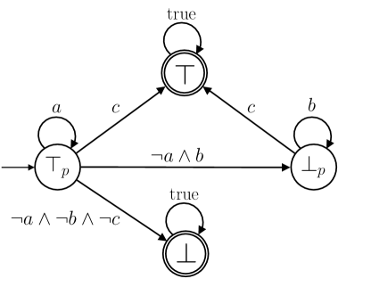
Figure 1: Ltl₄ monitor for property $\varphi=\mathbf{G}a\;\vee\;(b\,\mathbf{U}\,c)$.

2.3 Truth Values of LTL4-C

The objective of Ltl${}_{4}-$C is to verify the correctness of quantified properties at run time with respect to finite program traces. Such verification attempts to produce a sound verdict regardless of future continuations.

We incorporate six truth values to define the semantics of Ltl${}_{4}-$C: $\mathbb{B}_{6}=\{\top,\bot,{\top_{c}},{\bot_{c}},{\top_{p}},{\bot_{p}}\}$; true, false, currently true, currently false, presumably true, presumably false, respectively. The values in $\mathbb{B}_{6}$ form a lattice ordered as follows: $\bot<{\bot_{c}}<{\bot_{p}}<{\top_{p}}<{\top_{c}}<\top$. Given a finite trace $u$ and an Ltl${}_{4}-$C property $\varphi$, the informal description of evaluation of $u$ with respect to $\varphi$ is as follows:

• True ($\top$) denotes that any infinite extension of $u$ satisfies $\varphi$.

• False ($\bot$) denotes that any infinite extension of $u$ violates $\varphi$.

• Currently true (${\top_{c}}$) denotes that currently $u$ satisfies the counting quantifier constraint of $\varphi$, yet it is possible that a suffix of $u$ violates the constraint. For instance, the valuation of Property 1 (i.e., $\varphi_{1}$) is ${\top_{c}}$, if in a trace $u$, currently $50\%$ of files previously opened are closed. This is because (1) the inner Ltl property is permanently satisfied for at least $50\%$ of files previously opened, and (2) it is possible for a trace continuation to change this percentage to less than $50\%$ in the future (a trace in which enough new files are opened and not closed).

• Currently false (${\bot_{c}}$) denotes that currently $u$ violates the quantifier constraint of $\varphi$, yet it is possible that a suffix of $u$ satisfies the constraint. For instance, the valuation of Property 1 (i.e., $\varphi_{1}$) in a finite trace $u$ is ${\bot_{c}}$, if the number of files that were not successfully opened is currently greater than $50\%$. This could happen in the scenario where opening a file fails, possibly due to lack of permissions. Analogous to ${\top_{c}}$, the property is evaluated to ${\bot_{c}}$ because (1) the inner Ltl property is permanently satisfied for less than $50\%$ of files in the program trace, and (2) it is possible for a trace continuation to change this percentage to at least $50\%$ in the future.

Now let us consider modifying the property to support multiple open and close operations on the same file. For this purpose, we reformulate the property as follows:

$$\varphi_{2}=\mathbb{A}_{\geq 50\%}\,f:\textsf{\small intrace}(f)\Rightarrow\left(\mathbf{G}\left(\textsf{\small opened}(f)\,\mathbf{U}\,\textsf{\small close}(f)\right)\right)$$ (2)

• Presumably true (${\top_{p}}$) extends the definition of presumably true in Ltl₄ [4], where ${\top_{p}}$ denotes that $u$ satisfies the inner Ltl property and the counting quantifier constraint in $\varphi$, if the program terminates after execution of $u$. For example, Property 2 (i.e., $\varphi_{2}$) evaluates to ${\top_{p}}$, if at least $50\%$ of the files in the program trace are closed. Closed files presumably satisfy the property, since they satisfy the $\mathbf{G}$ operator thus far, yet can potentially violate it if the file is opened a subsequent time without being closed. Note that this property can never evaluate to ${\top_{c}}$, since no finite trace prefix can permanently satisfy the inner Ltl property. However, if the inner property can be permanently satisfied ($\top$) and presumably satisfied (${\top_{p}}$), then the entire Ltl${}_{4}-$C property can potentially evaluate to ${\top_{c}}$ if the numerical condition of the quantifier is satisfied. A property can evaluate to ${\top_{p}}$ only if the conditions for ${\top_{c}}$ are not met, since ${\top_{c}}$ is higher up the partial order of $\mathbb{B}_{6}$.

• Presumably false (${\bot_{p}}$) extends the definition of presumably false in Ltl₄ [4], which denotes that $u$ presumably violates the quantifier constraint in $\varphi$. According to the Property 2, this scenario will occur when the number of files that are either closed or opened and not yet closed is at least $50\%$ of all files in the trace. Opened files presumably violate the inner property, since closing the file is required but has not yet occurred. This condition should not conflict with ${\top_{p}}$ or ${\top_{c}}$, since they precede ${\bot_{p}}$ in the partial order of $\mathbb{B}_{6}$ and thus ${\bot_{p}}$ only occurs if the conditions for ${\top_{p}}$ and ${\top_{c}}$ do not hold.

2.4 Semantics of LTL4-C

An Ltl${}_{4}-$C property essentially defines a set of traces, where each traces is a sequences of events (i.e., sets of uninterpreted predicates). We define the semantics of Ltl${}_{4}-$C with respect to finite traces and present a method of utilizing these semantics for runtime verification. In the context of runtime verification, the objective is to ensure that a program trace (i.e., a sequence of sets of interpreted predicates) is in the set of traces that the property defines, given the interpretations of the property predicates within the program trace.

To introduce the semantics of Ltl${}_{4}-$C, we examine counting quantifiers further. Since the syntax of Ltl${}_{4}-$C allows nesting of counting quantifiers, a canonical form of properties is as follows:

$$\varphi=\mathbb{Q}_{\varphi}\;\psi$$ (3)

where $\psi$ is an Ltl property and $\mathbb{Q}_{\varphi}$ is a string of counting quantifiers

$$\mathbb{Q}_{\varphi}=\mathcal{Q}_{0}\mathcal{Q}_{1}\cdots\mathcal{Q}_{n-1}$$ (4)

such that each $\mathcal{Q}_{i}=\langle Q_{i},\sim_{i},c_{i},x_{i},p_{i}\rangle$, $0\leq i\leq n-1$, is a tuple encapsulating the counting quantifier information. That is, $Q_{i}\in\{\mathbb{A},\mathbb{E}\}$, $\sim_{i}\in\left\{<,\leq,>,\geq,=\right\}$, $c_{i}$ is the constraint constant, $x_{i}$ is the bound variable, and $p_{i}$ is the predicate within the quantifier (see Definition 3).

We presents semantics of Ltl${}_{4}-$C in a stepwise manner:

1. Variable valuation. First, we demonstrate how variable valuations are extracted from the trace and used to substitute variables in the formula.

2. Canonical variable valuations. Next, we demonstrate how to build a canonical structure of the variable valuations provided in Step 1. This canonical structure mirrors the canonical structure of Ltl${}_{4}-$C properties.

3. Valuation of property instances. A property instance is a unique substitution of variables in the property with values from their domains. This step demonstrate how to evaluate property instances.

4. Applying quantifier numerical constraints. This step demonstrates how to evaluate counting quantifiers by applying their numerical constraints on the valuation of a set of property instances from Step 3. The set of property instances is retrieved with respect to the canonical structure defined in Step 2.

5. Inductive semantics. Using the canonical structure in Step 2, and valuation of counting quantifiers in Step 4, we define semantics that begin at the outermost counting quantifier of an Ltl${}_{4}-$C property and evaluate quantifiers recursively inwards.

2.4.1 Variable Valuation

We define a vector $D_{\varphi}$ with respect to a property $\varphi$ as follows:

$$D_{\varphi}=\langle d_{0},d_{1},\cdots,d_{n-1}\rangle$$

where $n=|\mathbb{Q}_{\varphi}|$ and $d_{i}$, $0\leq i\leq n-1$, is a value for variable $x_{i}$. We denote the first $m$ components of the vector $D_{\varphi}$ (i.e., $\langle d_{0},d_{1},\cdots,d_{m-1}\rangle$) by $D_{\varphi}|^{m}$. We refer to $D_{\varphi}$ as a value vector and to $D_{\varphi}|^{m}$ as a partial value vector.

A property instances $\hat{\varphi}(D_{\varphi}|^{m})$ is obtained by replacing every occurrence of the variables $x_{0}\cdots x_{m-1}$ in $\varphi$ with the values $d_{0}\cdots d_{m-1}$, respectively. Thus, $\hat{\varphi}(D_{\varphi}|^{m})$ is free of quantifiers of index less than $m$, yet remains quantified over variables $x_{m}\cdots x_{n-1}$. For instance, for the following property

$$\varphi=\mathbb{A}_{>c_{1}}\,x:p_{x}(x)\Rightarrow\left(\mathbb{A}_{<c_{2}}\,y:p_{y}(y)\Rightarrow\mathbf{G}\,q(x,y)\right)$$

and value vector $D_{\varphi}=\langle 1,2\rangle$ (i.e., the vector of values for variables $x$ and $y$, respectively), $\hat{\varphi}(D_{\varphi})$ will be

$$\hat{\varphi}(\langle 1,2\rangle)=p_{x}(1)\Rightarrow\left(p_{y}(2)\Rightarrow\mathbf{G}\,q(1,2)\right)$$

We now define the set $\mathbb{D}_{\varphi,u}$ as the set of all value vectors with respect to a property $\varphi=\mathbb{Q}_{\varphi}\;\psi$ and a finite trace $u=u_{0}u_{1}\cdots u_{k}$:

$$\mathbb{D}_{\varphi,u}=\{D_{\varphi}\mid\exists j\in[0,k]:\forall i\in[0,n-1]:p_{i}(d_{i})\in u_{j}\}$$ (5)

where $n=|\mathbb{Q}_{\varphi}|$.

2.4.2 Canonical Variable Valuations

An Ltl${}_{4}-$C property follows a canonical structure, in which every counting quantifier $\mathcal{Q}_{i}$ has a parent quantifier $\mathcal{Q}_{i-1}$, except for $\mathcal{Q}_{0}$ which is the root counting quantifier. A counting quantifier $\mathcal{Q}_{i}$ is applied over all valuations of its variable $x_{i}$ given a unique valuation of its predecessor variables $x_{0},\cdots,x_{i-1}$. Hence, we define function $\mathcal{P}$ which takes as input a partial value vector $D_{\varphi}|^{m}$, and returns all partial value vectors in $\mathbb{D}_{\varphi,u}$ of length $m+1$, such that the first $m$ elements of these vectors is the same as $D_{\varphi}|^{m}$. In this context, we refer to $D_{\varphi}|^{m}$ as a parent vector and all the returned vectors as child vectors. Similarly, a property instance can have a parent; for instance, $\hat{\varphi}(D_{\varphi}|^{m})$ is the parent of $\hat{\varphi}(D_{\varphi}|^{m+1})$.

$$\mathcal{P}(\varphi,u,D_{\varphi}|^{m})=\bigg{\{}D_{\varphi}^{\prime}|^{m+1}\;\bigg{|}\;D_{\varphi}^{\prime}\in\mathbb{D}_{\varphi,u}\,\wedge\,D_{\varphi}^{\prime}|^{m}=D_{\varphi}|^{m}\bigg{\}}$$

Following the example above, assume there are two value vectors: $\langle 1,2\rangle$ and $\langle 1,3\rangle$. In this case,

$$\mathcal{P}(\varphi,u,\langle 1\rangle)=\big{\{}\langle 1,2\rangle,\langle 1,3\rangle\big{\}}$$

2.4.3 Valuation of Property Instances

As per the definition of $\mathbb{D}_{\varphi,u}$, every value vector $D_{\varphi}=\langle d_{0}\cdots d_{n-1}\rangle$ in $\mathbb{D}_{\varphi,u}$ contains values for which the predicates $p_{i}(d_{i})$ hold in some trace event $u_{j}$. For simplicity, we denote this as a value vector in a trace event $u_{j}$. These value vectors can possibly be in multiple and interleaved events in the trace. Thus, we define a trace $u^{D_{\varphi}}=u^{D_{\varphi}}_{0}u^{D_{\varphi}}_{1}\cdots u^{D_{\varphi}}_{l}$ as a subsequence of the trace $u$ such that the value vector $D_{\varphi}$ is in every event:

$$\forall\,j\in[0,l]:\forall\,i\in[0,n-1]:p_{i}(d_{i})\in u^{D_{\varphi}}_{j}$$

For any property instance $\hat{\varphi}(D_{\varphi})$, we wish to evaluate $[u^{D_{\varphi}}\models_{6}\hat{\varphi}(D_{\varphi})]$ (read as valuation of $\hat{\varphi}(D_{\varphi})$ with respect to $u^{D_{\varphi}}$ for Ltl${}_{4}-$C), since any other event in trace $u$ is not of interest to $\hat{\varphi}(D_{\varphi})$.

By leveraging $u^{D_{\varphi}}$, we define function $\mathcal{B}$ as follows:

$\mathcal{B}(\varphi,u,D_{\varphi}|^{m},b)=$

$$\begin{cases}D_{\varphi}^{\prime}|^{m+1}\in\mathcal{P}(\varphi,u,D_{\varphi}|^{m})\mid&\\ \quad[u^{D_{\varphi}^{\prime}|^{m+1}}\models_{6}\hat{\varphi}(D_{\varphi}^{\prime}|^{m+1})]=b&\text{iff}~{}m<|\mathbb{Q}_{\varphi}|-1\\ D_{\varphi}^{\prime}|^{m+1}\in\mathcal{P}(\varphi,u,D_{\varphi}|^{m})\mid&\\ \quad[u^{D_{\varphi}^{\prime}|^{m+1}}\models_{4}\hat{\varphi}(D_{\varphi}^{\prime}|^{m+1})]=b&\text{iff}~{}m=|\mathbb{Q}_{\varphi}|-1\\ \end{cases}$$

where $b$ is a truth value in $\mathbb{B}_{6}$. Function $\mathcal{B}$ can be implemented in a straightforward manner, where it iterates over all its children value vectors $D_{\varphi}^{\prime}|^{m+1}$ which are retrieved using $\mathcal{P}$. For every child vector, the function checks whether $\hat{\varphi}(D_{\varphi}^{\prime}|^{m+1})$ evaluates to $b$ with respect to the trace subsequence $u^{D_{\varphi}^{\prime}|^{m+1}}$.

To clarify $\mathcal{B}$, let us refer to our example earlier. Let a program trace $u$ be as follows:

$$u=\{p_{x}(1),p_{y}(2),\cdots\},\{p_{x}(1),p_{y}(3),\cdots\},\{p_{x}(1),p_{y}(2),\cdots\}$$

With respect to this trace, $\mathcal{P}(\varphi,u,\langle 1\rangle)=\{\langle 1,2\rangle,\langle 1,3\rangle\}$. As per the definition of $u^{D_{\varphi}}$, $u^{\langle 1,2\rangle}=u_{0}u_{2}$, and $u^{\langle 1,3\rangle}=u_{1}$. Thus, $\mathcal{B}(\varphi,u,\langle 1\rangle,b)$ checks the following:

$$[u^{\langle 1,2\rangle} \models_{4}p_{x}(1)\Rightarrow\left(p_{y}(2)\Rightarrow\mathbf{G}\,q(1,2)\right)]=b$$

$$[u^{\langle 1,3\rangle} \models_{4}p_{x}(1)\Rightarrow\left(p_{y}(3)\Rightarrow\mathbf{G}\,q(1,3)\right)]=b$$

The definition of $u^{D_{\varphi}}$ implies that $p_{i}(d_{i})\in u^{D_{\varphi}}_{j}$ for all $j$. Thus, we can simplify the property by omitting the $p$ predicates since they hold by definition:

$$[u^{\langle 1,2\rangle} \models_{4}\mathbf{G}\,q(1,2)]=b$$

$$[u^{\langle 1,3\rangle} \models_{4}\mathbf{G}\,q(1,3)]=b$$

For instance, if only $[u^{\langle 1,2\rangle}\models_{4}\mathbf{G}\,q(1,2)]=b$ holds, then

$$\mathcal{B}(\varphi,u,\langle 1\rangle,b)=\{\langle 1,2\rangle\}$$

As can be seen in the example, the property instances that are evaluated are Ltl₄ properties. This is because the input to $\mathcal{B}$ is $D_{\varphi}|^{1}=D_{\varphi}|^{|\mathbb{Q}_{\varphi}|-1}$, which represents the inner most quantifier.

2.4.4 Applying Quantifier Numerical Constraints

Finally, numerical constraints should be incorporated in the semantics. We define function $\mathcal{S}$ as follows:

$$\small\mathcal{S}(\varphi,u,D_{\varphi}|^{m},B)=\begin{cases}\vphantom{\Bigg{|}}\bigg{|}\bigcup\limits_{b\in B}{\mathcal{B}(\varphi,u,D_{\varphi}|^{m},b)}\bigg{|}\sim_{i}\\ \quad c_{i}\times|\{\mathcal{P}(\varphi,u,D_{\varphi}|^{m})\}|&\text{iff }Q_{m}=\mathbb{A}\\ \vphantom{\Bigg{|}}\bigg{|}\bigcup\limits_{b\in B}{\mathcal{B}(\varphi,u,D_{\varphi}|^{m},b)}\bigg{|}\sim_{i}c_{i}&\text{iff }Q_{m}=\mathbb{E}\end{cases}$$ (6)

where $B\subseteq\mathbb{B}_{6}$ is a set of truth values. This function returns whether a counting quantifier constraint is satisfied or not based on any of the truth values $b\in B$. Observe that, for percentage counting quantifiers, the constraint value denotes the percentage of property instances that evaluate to $b$. For instance counting quantifiers, the constraint value denotes the number of property instances that evaluate to $b$. For instance, consider Property 7 which is read as: for all users, there exists at most $3$ requests of type login that end with an unauthorized status. For such a property, if $4$ or more unauthorized login attempts are detected for the same user, the property is permanently violated.

2.4.5 Inductive Semantics

Using the previously defined set of of functions, we now formalize Ltl${}_{4}-$C semantics.

Definition 7 (Ltl${}_{4}-$C Semantics)

Ltl${}_{4}-$C semantics for properties with counting quantifiers are defined as follows:

$$[u\models_{6}\varphi]=\begin{cases}\top&\text{iff }\;\;\mathcal{S}(\varphi,u,\langle\rangle,\{\top\})=1\;\wedge\\ &\forall v\in\Sigma^{\omega}:[uv\models_{6}\varphi]=\top\\ \bot&\text{iff}\;\;\mathcal{S}(\varphi,u,\langle\rangle,\mathbb{B}_{6}-\{\bot\})=0\;\wedge\\ &\forall v\in\Sigma^{\omega}:[uv\models_{6}\varphi]=\bot\\ {\top_{c}}&\text{iff}\;\;\mathcal{S}(\varphi,u,\langle\rangle,\{\top,{\top_{c}}\})=1\;\wedge\\ &\exists v\in\Sigma^{\omega}:[uv\models_{6}\varphi]\neq{\top_{c}}\\ {\bot_{c}}&\text{iff }\;\;\mathcal{S}(\varphi,u,\langle\rangle,\mathbb{B}_{6}-\{\bot,{\bot_{c}}\})=0\;\wedge\\ &\exists v\in\Sigma^{\omega}:[uv\models_{6}\varphi]\neq{\bot_{c}}\\ {\top_{p}}&\text{iff }\;\;\mathcal{S}(\varphi,u,\langle\rangle,\{\top,{\top_{c}},{\top_{p}}\})=1\;\wedge\\ &\mathcal{S}(\varphi,u,\langle\rangle,\{\top,{\top_{c}}\})=0\\ {\bot_{p}}&\text{iff }\;\;\mathcal{S}(\varphi,u,\langle\rangle,\{\top,{\top_{c}},{\top_{p}}\})=0\;\wedge\\ &\mathcal{S}(\varphi,u,\langle\rangle,\mathbb{B}_{6}-\{\bot,{\bot_{c}}\})=0~{}\blacksquare\end{cases}$$

Note that these semantics are applied recursively until there is only one counting quantifier left in the formula, at which point $\mathcal{B}$ checks the valuation based on Ltl₄ semantics ($[u^{D_{\varphi}}\models_{4}\hat{\varphi}(D_{\varphi})]=b$). When checking the valuation of these Ltl₄ properties, $\mathcal{B}$ will always return an empty set in case the input $b$ is ${\top_{c}}$ or ${\bot_{c}}$, since these truth values are inapplicable to Ltl₄ properties. As mentioned earlier, truth values in $\mathbb{B}_{6}$ form a lattice. Standard lattice operators $\sqcap$ and $\sqcup$ are defined as expected based on the lattice’s partial order. Permanent satisfaction $(\top)$ or violation $(\bot)$ is applicable to $\mathbb{E}$ quantifiers regardless of the comparison operator, as well as a special case of $\mathbb{A}$ quantifiers:

• $\mathbb{A}$ quantifier. As mentioned earlier, if the $\mathbb{A}$ quantifier is not subscripted, it is assumed to denote $\mathbb{A}_{=1}$. In this case, a single violation in its child property instances causes a permanent violation of the quantified property.

• $\mathbb{E}$ quantifier. Permanent violation is possible for any numerical constraint attached to an $\mathbb{E}$ quantifier, since it is a condition on the number of satisfied property instances.

Property 7 illustrates an example of an $\mathbb{E}$ quantifier that can be permanently violated. Also, since the $\mathbb{A}$ quantifier in Property 7 defaults to $\mathbb{A}_{=1}$, it will be violated if a single user makes more than three unauthorized login attempts. In such a case, the entire property evaluates to $\bot$. Table 1 illustrates how permanent satisfaction or violation apply to the different numerical constraints of $\mathbb{E}$ quantifiers.

$$\mathbb{A}x:\textsf{\small user}(x)\Rightarrow\left(\mathbb{E}_{\leq 3}\,r:\textsf{\small rid}(r)\Rightarrow\left(\textsf{\small login}\wedge\textsf{\small unauthorized}\right)\right)$$ (7)

Table 1: Rules of permanent satisfaction or violation of $\mathbb{E}$ constraints

Operator	Verdict
$>c$	Permanent satisfaction if $>c$
$\geq c$	Permanent satisfaction if $\geq c$
$=c$	Permanent violation if $>c$
$<c$	Permanent violation if $\geq c$
$\leq c$	Permanent violation if $>c$

To clarify the semantics, consider Property 7 and the following program trace:

$$\{\textsf{\small rid}(12),\textsf{\small user}(Adam),\textsf{\small login},\textsf{\small unauthorized}\}$$

$$\{\textsf{\small rid}(13),\textsf{\small user}(Adam),\textsf{\small login},\textsf{\small unauthorized}\}$$

$$\{\textsf{\small rid}(14),\textsf{\small user}(Jack),\textsf{\small login},\textsf{\small authorized}\}$$

$$\{\textsf{\small rid}(15),\textsf{\small user}(Adam),\textsf{\small login},\textsf{\small unauthorized}\}$$

$$\{\textsf{\small rid}(16),\textsf{\small user}(Adam),\textsf{\small login},\textsf{\small unauthorized}\}$$

where each line represents an event: a set of interpreted predicates. Each event contains a request identifier (rid), a username, a request type (login), and response status (authorized or unauthorized). As seen in the trace, there are $5$ distinct value vectors: $\langle Adam,12\rangle$, $\langle Adam,13\rangle$, $\langle Jack,14\rangle$, $\langle Adam,15\rangle$, and $\langle Adam,16\rangle$. Now, let us apply the inductive semantics on the property.

Step 1. We begin by checking the truth value of $[u\models_{6}\varphi]$, which requires determining which condition in Definition 7 applies. This requires the evaluation of function $\mathcal{S}$ for the different truth values shown. Since we are verifying $\varphi$, we begin with the outermost counting quantifier, which is a $\mathbb{A}$ quantifier. Thus, $\mathcal{S}$ will require calculating the cardinality of the set $\mathcal{P}(\varphi,u,D_{\varphi}|^{0})$, which in case of the trace should be $|\{Adam,Jack\}|=2$. Now, in order to evaluate $\mathcal{S}$, one has to evaluate $\mathcal{B}$ to determine whether each property instance evaluates to a certain truth value or not. The two property instances thus far are:

$$\hat{\varphi}(D_{\varphi}|^{1}) =\hat{\varphi}(Adam)=\mathbb{E}_{\leq 3}\,r:\textsf{\small rid}(r)\Rightarrow\left(\textsf{\small login}\wedge\textsf{\small unauthorized}\right)$$

$$\hat{\varphi}(D_{\varphi}^{\prime}|^{1}) =\hat{\varphi}(Jack)=\mathbb{E}_{\leq 3}\,r:\textsf{\small rid}(r)\Rightarrow\left(\textsf{\small login}\wedge\textsf{\small unauthorized}\right)$$

And the trace subsequences for these property instances respectively are:

$$u^{D_{\varphi}|^{1}}= \{\textsf{\small rid}(12),\cdots\}\{\textsf{\small rid}(13),\cdots\}\{\textsf{\small rid}(15),\cdots\}\{\textsf{\small rid}(16),\cdots\}$$

$$u^{D_{\varphi}^{\prime}|^{1}}= \{\textsf{\small rid}(14),\cdots\}$$

Note that $\textsf{\small user}(Adam)\Rightarrow\cdots$ is omitted from $\hat{\varphi}(D_{\varphi}|^{1})$ since $\textsf{\small user}(Adam)$ holds according to the trace subsequence. The same applies to $\textsf{\small user}(Jack)$. Evaluating these property instances with respect to the trace subsequences requires referring to Definition 7 again, which marks the second level of recursion.

Step 2. Let us consider the property instance $\hat{\varphi}(D_{\varphi}|^{1})$, which begins with an $\mathbb{E}$ quantifier and has Ltl₄ properties as child instances (refer to $\mathcal{P}$). These properties are in the form of $\textsf{\small login}\,\wedge\,\textsf{\small unauthorized}$, where there is one instance for each distinct request identifier. We can deduce that the property holds for all $4$ requests: $12$, $13$, $15$, and $16$, thus evaluating to $\top$. Therefore, the following holds:

$$\mathcal{B}(\hat{\varphi}(D_{\varphi}|^{1}),u^{D_{\varphi}|^{1}},D_{\varphi}|^{1},\top)=4$$

This value, when used in $\mathcal{S}(\hat{\varphi}(D_{\varphi}|^{1}),u^{D_{\varphi}|^{1}},D_{\varphi}|^{1},\{\top\})$ will violate the numerical condition: $4\not\leq 3$, resulting in $\mathcal{S}$ valuating to $0$ (false). Based on the conditions in Definition 7 and the rules of permanent violation, this property instance becomes permanently violated and thus the verdict is $\bot$.

The other property instance $\hat{\varphi}(D_{\varphi}^{\prime}|^{1})$ will however evaluate to $\top$ since its child property instance

$$\hat{\varphi}(D_{\varphi}^{\prime}|^{2})=\hat{\varphi}(\langle Jack,14\rangle)=\textsf{\small login}\,\wedge\,\textsf{\small unauthorized}$$

is violated, and thus the number of satisfied instances is still less than $3$.

Step 3. In this step we use the valuations determined in Step 2 to produce verdicts for the property instances in Step 1. Based on $\mathcal{S}$, the $\mathbb{A}$ quantifier’s numerical condition is violated, since not all instances are satisfied. The final verdict should thus be $[u\models_{6}\varphi]=\bot$, which denotes a permanent violation of the property.

3 Divide-and-Conquer-based
Monitoring of LTL4-C

In this section, we describe our technique inspired by divide-and-conquer for evaluating Ltl${}_{4}-$C properties at run time. This approach forms the basis of our parallel verification algorithm in Section 4.

Unlike runtime verification of propositional Ltl₄ properties, where the structure of a monitor is determined solely based on the property itself, a monitor for an Ltl${}_{4}-$C needs to evolve at run time, since the valuation of quantified variables change over time. More specifically, the monitor $\mathcal{M}_{\varphi}$ for an Ltl${}_{4}-$C property $\varphi=\mathbb{Q}_{\varphi}\psi$ relies on instantiating a submonitor for each property instance $\hat{\varphi}$ obtained at run time. We incorporate two type of submonitors: (1) Ltl₄ submonitors evaluate the inner Ltl property $\psi$, and (2) quantifier submonitors deal with quantifiers in $\mathbb{Q}_{\varphi}$, described in Subsections 3.1 and 3.2. In Subsection 3.3, we explain the conditions under which a submonitor is instantiated at run time. Finally, in Subsection 3.4, we elaborate on how submonitors evaluate an Ltl${}_{4}-$C property.

3.1 LTL4 Submonitors

Let $\varphi=\mathbb{Q}_{\varphi}\psi$ be an Ltl${}_{4}-$C property. If $|\mathbb{Q}_{\varphi}|=0$ (respectively, one wants to evaluate $\hat{\varphi}(D_{\varphi}|^{i})$, where $i=|\mathbb{Q}_{\varphi}|$), then $\varphi$ (respectively, $\hat{\varphi}(D_{\varphi}|^{i})$) is free of quantifiers and, thus, the monitor (respectively, submonitor) of such a property is a standard Ltl₄ monitor (see Definition 6). We denote Ltl₄ submonitors as $\mathcal{M}^{*}_{D_{\varphi}}$, where $D_{\varphi}$ is the value vector with which the monitor is initialized.

3.2 Quantifier Submonitors

Given a finite trace $u$ and an Ltl${}_{4}-$C property $\varphi=\mathbb{Q}_{\varphi}\psi$, a quantifier submonitor ($\mathcal{M}^{\mathcal{Q}}$) is a monitor responsible for determining the valuation of a property instance $\hat{\varphi}(D_{\varphi}|^{i})$ with respect to a trace subsequence $u^{D_{\varphi}|^{i}}$, if $i<|\mathbb{Q}_{\varphi}|$. Obviously, such a valuation is in $\mathbb{B}_{6}$. Let $\mathbb{V}$ be a six-dimensional vector space, where each dimension represents a truth value in $\mathbb{B}_{6}$.

Definition 8 (Quantifier Submonitor)

Let $\varphi=\mathbb{Q}_{\varphi}\psi$ be an Ltl${}_{4}-$C property and $\hat{\varphi}(D_{\varphi}|^{i})$ be a property instance, with $i\in[0,|\mathbb{Q}_{\varphi}|-1]$. The quantifier submonitor for $\hat{\varphi}(D_{\varphi}|^{i})$ is the tuple $\mathcal{M}_{D_{\varphi}|^{i}}^{\mathcal{Q}}=\langle\mathcal{Q}_{i},\mathbb{M}_{D_{\varphi}|^{i}},v,b\rangle$, where

• $\mathcal{Q}_{i}$ encapsulates the quantifier information (see Equation 4)

• $v\in\mathbb{V}$ represents the current number of child property instances that evaluate to each truth value in $\mathbb{B}_{6}$ with respect to their trace subsequences,

• $b\in\mathbb{B}_{6}$ is the current value of ${[u^{D_{\varphi}|^{i}}\models_{6}\hat{\varphi}(D_{\varphi}|^{i})]}$,

• $\mathbb{M}_{D_{\varphi}|^{i}}$ is the set of child submonitors (submonitors of child property instances) defined as follows:

  $$\mathbb{M}_{D_{\varphi}|^{i}}=\begin{cases}\{\mathcal{M}^{*}_{D_{\varphi}^{\prime}}\mid D_{\varphi}^{\prime}|^{i}=D_{\varphi}|^{i}\}&\text{if }i=|\mathbb{Q}_{\varphi}|-1\\ \{\mathcal{M}^{\mathcal{Q}}_{D_{\varphi}^{\prime}|^{i+1}}\mid D_{\varphi}^{\prime}|^{i}=D_{\varphi}|^{i}\}&\text{if }i<|\mathbb{Q}_{\varphi}|-1\end{cases}$$

Thus, if $i=|\mathbb{Q}_{\varphi}|-1$, all child submonitors are Ltl₄ submonitors. Otherwise, they are quantifier submonitors of the respective child property instances.$~{}\blacksquare$

Based on the definition, every quantifier submonitor references a set of child monitors. We use the following notation to denote a hierarchy of a submonitor and its children:

$$\mathcal{M}^{\mathcal{Q}}_{D_{\varphi}|^{i}}\big{\{}\mathcal{M}^{\mathcal{Q}}_{D_{\varphi}|^{i+1}},\mathcal{M}^{\mathcal{Q}}_{D_{\varphi}^{\prime}|^{i+1}},\mathcal{M}^{\mathcal{Q}}_{D_{\varphi}^{\prime\prime}|^{i+1}},\cdots\big{\}}$$

such that $D_{\varphi}|^{i}=D_{\varphi}^{\prime}|^{i}=D_{\varphi}^{\prime\prime}|^{i}\cdots$ and $i<|\mathbb{Q}_{\varphi}|-1$ which is why the child monitors are quantifier submonitors.

3.3 Instantiating Submonitors

Let an Ltl${}_{4}-$C monitor $\mathcal{M}_{\varphi}$ for property $\varphi$ evaluate the property with respect to a finite trace $u=u_{0}u_{1}\cdots$. Let $D_{\varphi}=\langle d_{0},d_{1},\cdots\rangle$ be a value vector and $u_{k}$ the first trace event such that $\forall d_{i}:p_{i}(d_{i})\in u_{k}$, where $p_{i}$ is the predicate within each quantifier (i.e. $\mathbb{A}x_{i}:p_{i}(x_{i})\Rightarrow\cdots$). In this case, the Ltl${}_{4}-$C monitor instantiates submonitors for every property instance resulting from that value vector. A value vector of length $|\mathbb{Q}_{\varphi}|$ results in $|\mathbb{Q}_{\varphi}|+1$ property instances: one for each quantifier in addition to an Ltl₄ inner property. The hierarchy of the instantiated submonitors is as follows:

$$\mathcal{M}^{\mathcal{Q}}_{D_{\varphi}|^{0}}\bigg{\{}\mathcal{M}^{\mathcal{Q}}_{D_{\varphi}|^{1}}\Big{\{}\cdots\big{\{}\mathcal{M}^{\mathcal{Q}}_{D_{\varphi}|^{|\mathbb{Q}_{\varphi}-1|}}\{\mathcal{M}^{*}_{D_{\varphi}}\}\big{\}}\Big{\}}\bigg{\}}$$

If another value vector $D_{\varphi}^{\prime}$ is subsequently encountered for the first time, the hierarchy of submonitors becomes as follows:

$$\mathcal{M}^{\mathcal{Q}}_{D_{\varphi}|^{0}}\Big{\{}\mathcal{M}^{\mathcal{Q}}_{D_{\varphi}|^{1}}\big{\{}\cdots\{\mathcal{M}^{*}_{D_{\varphi}}\}\big{\}},\mathcal{M}^{\mathcal{Q}}_{D_{\varphi}^{\prime}|^{1}}\big{\{}\cdots\{\mathcal{M}^{*}_{D_{\varphi}^{\prime}}\}\Big{\}}$$

Since the hierarchy is formulated as a recursive set, no duplicate submonitors are allowed. Two submonitors are duplicates, if they represent identical value vectors. If $D_{\varphi}|^{1}=D_{\varphi}^{\prime}|^{1}$, the respective monitors are merged. Such merging is explained in detail in Section 4.

3.4 Evaluating LTL4-C Properties

Once the Ltl${}_{4}-$C monitor instantiates its submonitors, every submonitor is responsible for updating its truth value. The truth value of Ltl₄ submonitors ($\mathcal{M}^{*}$) maps to the current state of the submonitor’s automaton as described in Definition 6. Quantifier submonitors update their truth value based on the truth values of all child submonitors. The number of child submonitors whose truth value is $\top$ is stored in $v_{\top}$ (i.e., the $\top$ dimension of vector $v$) and so on for all truth values in $\mathbb{B}_{6}$. Then, Ltl${}_{4}-$C semantics are applied, beginning with function $\mathcal{S}$ (see Equation 6), which in turn relies on the cardinality of function $\mathcal{B}(\varphi,u,D_{\varphi}|^{i},b)$ where $b$ is a truth value. This cardinality is readily provided by the vector $v$, such that for instance $\mathcal{B}(\varphi,u,D_{\varphi}|^{i},\top)=v_{\top}$ and so on.

Since each submonitor depends on its child submonitors, updating truth values proceeds outwards, starting at Ltl₄ submonitors, then recursively parent submonitors update their truth values until the submonitor $\mathcal{M}^{\mathcal{Q}}_{D_{\varphi}|^{0}}$, which is the root submonitor. The truth value of the root submonitor is the truth value of property $\varphi$ with respect to trace $u$. This is visualized as the tree shown in Figure 2.

Figure 2: Tree structure of an Ltl${}_{4}-$C monitor.

4 Parallel Algorithm Design

The main challenge in designing a runtime monitor is to ensure that its behavior does not intervene with functional and extra-functional (e.g., timing constraints) behavior of the program under scrutiny. This section presents a parallel algorithm for verification of Ltl${}_{4}-$C properties. Our idea is that such a parallel algorithm enables us to offload the monitoring tasks into a different computing unit (e.g., the GPU). The algorithm utilizes the popular MapReduce technique to spawn and merge submonitors to determine the final verdict. This section is organized as follows: Subsection 4.1 describes how valuations are extracted from a trace in run time, and Subsection 4.2 describes the steps of the algorithm in detail.

4.1 Valuation Extraction

Valuation extraction refers to obtaining a valuation of quantified variables from the trace. As described in Ltl${}_{4}-$C semantics, the predicate $p_{i}(x_{i})$ identifies the subset of the domain of $x_{i}$ over which the quantifier is applied: namely the subset that exists in the trace. From a theoretical perspective, we check whether the predicate is a member of some trace event, which is a set of predicates. From an implementation perspective, the trace event is a key-value structure, where the key is for instance a string identifying the quantified variable, and the value is the concrete value of the quantified variable in that trace event. Consider the following property:

$$\varphi=\mathbb{A}_{\geq 0.95}\,s\,\text{:}\,\textsf{\small socket}(s)\Rightarrow\left(\mathbf{G}\,\textsf{\small recv}\left(s\right)\Rightarrow\textbf{F}\,\textsf{\small respond}\left(s\right)\right)$$ (8)

Predicate $p$ in this case is $\textsf{\small socket}(s)$, and a trace event should contain a key socket and a value $\in[0,65535]$ representing the socket file descriptor in the system. Thus, the valuation extraction function $\varepsilon(u_{i},K)=D_{\varphi}$ returns a map where keys are in $K$, and the value of each key is the value of the quantified variable corresponding to this key. These keys are defined by the user.

4.2 Algorithm Steps

Algorithm 1 presents the pseudocode of the parallel monitoring algorithm. Given an Ltl${}_{4}-$C property $\varphi=\mathbb{Q}_{\varphi}\,\psi$, the input to the algorithm is the Ltl₄ monitor $\mathcal{M}^{*}$ of Ltl₄ property $\psi$, a finite trace $u$, the set of quantifiers $\mathbb{Q}_{\varphi}$, and the vector of keys $K$ used to extract valuations. Note that the algorithm supports both online and offline runtime verification. Offline mode is straightforward since the algorithm receives a finite trace that it can evaluate. In the case of online mode, the algorithm maintains data structures that represent the tree structure shown in Figure 2, and repeated invocation of the algorithm updates these data structures incrementally. Thus, a monitoring solution can invoke the algorithm periodically or based on same event in an online fashion, and still receive an evolving verdict.

The entry point to the algorithm is at Line 5 which is invoked when the monitor receives a trace to process. The algorithm returns a truth value of the property at Line 8. Subsections 4.2.1 – 4.2.4 describe the functional calls between Lines 5 – 8. The MapReduce operations are visible in functions SortTrace and ApplyQuantifiers, which perform a map ($\rightrightarrows$) in Lines 10 and 51 respectively. ApplyQuantifiers also performs a reduction ($\rightarrowtail$) in Line 52.

4.2.1 Trace Sorting

As shown in Algorithm 1, the first step in the algorithm is to sort the input trace $u$ (Line 5). The function SortTrace performs this functionality as follows:

1. The function performs a parallel map of every trace event to the value vector that it holds using $\varepsilon$ (Line 10).

2. The mapped trace is sorted in parallel using the quantifier variable keys (Line 11). For instance, according to Property 8, the key used for sorting will be socket, effectively sorting the trace by socket identifier.

3. The sorted trace is then compacted based on valuations, and the function returns a map $\mu$ where keys are value vectors and values are the ranges of where these value vectors exist in trace $u$ (Line 12). A range contains the start and end index. This essentially defines the subsequences $u^{D_{\varphi}}$ for each property instance $\hat{\varphi}(D_{\varphi})$ (refer to Subsection 2.4).

4.2.2 Monitor Spawning

Monitor spawning is the second step of the algorithm (Line 6). The function SpawnMonitors receives a map $\mu$ and searches the cached collection of previously encountered value vectors $\mathbb{D}$ for duplicates. If a value vector in $\mu$ is new, it creates submonitors and inserts them in the tree of submonitors $T$ (Line 19). The function AddToTree attempts to generate $|\mathbb{Q}_{\varphi}|-1$ quantifier submonitors $\mathcal{M}^{\mathcal{Q}}$ (Line 26) ensuring there are no duplicate monitors in the tree (Line 27). After all quantifier submonitors are created, SpawnMonitors creates an Ltl₄ submonitor $\mathcal{M}^{*}$ and adds it as a child to the leaf quantifier submonitor in the tree representing the value vector (Line 20). This resembles the structure in Figure 2. Creation of submonitors is performed in parallel for all value vectors in trace $u$.

4.2.3 Distributing the Trace

The next step in the algorithm is to distribute the sorted trace to all Ltl₄ submonitors (Line 7). The function Distribute instructs every Ltl₄ submonitor to process its respective trace by passing the full trace and the range of its respective subsequence, which is provided by the map $\mu$ (Line 42). The Ltl₄ monitor updates its state according to the trace subsequence and stores its truth value $b$.

4.2.4 Applying Quantifiers

Applying quantifiers is a recursive process, beginning with the leaf quantifier submonitors and proceeding upwards towards the root of the tree (Line 8). Function ApplyQuantifiers operates in the following steps:

1. The function retrieves all quantifier submonitors at the $i^{th}$ level in the tree $T$ (Line 50).

2. In parallel, for each quantifier submonitor, all child submonitor truth values are reduced into a single truth value of that quantifier submonitor (Lines 51-53). This step essentially reduces all child truth vectors into a single vector and then applies Ltl${}_{4}-$C semantics to determine the truth value of the current submonitor.

3. The function proceeds recursively calling itself on submonitors that are one level higher. It terminates when the root of the tree is reached, where the truth value is the final verdict of the property with respect to the trace.

1:INPUT: An Ltl₄ monitor $\mathcal{M}^{*}$ of Ltl property $\psi$, a finite trace $u$, a set of quantifiers $\mathbb{Q}_{\varphi}$, and a vector of keys $K$ to extract valuations of quantified variables.

2:declare $T=\{\mathcal{M}^{\mathcal{Q}}_{D|^{0}}\}$ $\triangleright$ Tree of quantifier submonitors

3:declare $\mathbb{D}=\{\}$ $\triangleright$ Value vector set

4:declare $\mathbb{M}^{*}=\{\}$ $\triangleright$ Ltl₄ submonitor set

5:$\mu\leftarrow$ SortTrace($u$) $\triangleright$ The entry point

6:SpawnMonitors($\mu$)

7:Distribute($u$,$\mu$)

8:return ApplyQuantifiers($|\mathbb{Q}_{\varphi}-1|$)  

9:function SortTrace($u$)$\triangleright$ Trace sorting and compaction

10:    $u_{i}\rightrightarrows u^{\prime}_{i}:=\varepsilon(u_{i},K)$ $\triangleright$ $\parallel$ map to value vectors

11:    ParallelSort($u^{\prime}$,$K$)

12:    $\mu\langle D,r\rangle\leftarrow$ ParallelCompact($u^{\prime}$)

13:    return $\mu$

14:end function 

15:function SpawnMonitors($\mu$)$\triangleright$ Monitor spawning

16:    for $D\in\mu$ do in parallel

17:       if $D\not\in\mathbb{D}$ then

18:          Add($\mathbb{D}$,$D$)

19:          $t\leftarrow$ AddToTree($D$)

20:          $t$.addMonitor(CreateMonitor($D$))

21:       end if

22:    end for

23:end function 

24:function AddToTree($D$)

25:    $t$ = $T$.root

26:    for $i\in[1,|\mathbb{Q}_{\varphi}|-1]$ do

27:       if $\mathcal{M}^{\mathcal{Q}}_{D|^{i}}\not\in t$.children then

28:          $t$.addchild($\mathcal{M}^{\mathcal{Q}}_{D|^{i}}$)

29:       end if

30:       $t\leftarrow t$.children$\left[\mathcal{M}^{\mathcal{Q}}_{D|^{i}}\right]$

31:    end for

32:    return $t$

33:end function 

34:function CreateMonitor($D$)$\triangleright$ Monitor creation

35:    $\mathcal{M}^{*}_{D}\leftarrow$ LaunchMonitorThread($D$)

36:    $\mathcal{M}^{*}_{D}.D\leftarrow D$

37:    add($\mathbb{M}^{*}$,$\mathcal{M}^{*}_{D}$)

38:    return $\mathcal{M}^{*}_{D}$

39:end function 

40:function Distribute($u$,$\mu$)$\triangleright$ Distribute trace to monitors

41:    for $\mathcal{M}^{*}_{D}\in\mathbb{M}^{*}$ do in parallel

42:       ProcessBuffer($\mathcal{M}^{*}_{D}$,$u$,$\mu[\mathcal{M}^{*}_{D}.D]$)

43:    end for

44:end function 

45:function ProcessBuffer($\mathcal{M}^{*}_{D}$,$u$,$r$)$\triangleright$ Process trace subsequence

46:    filter include $u\rightrightarrows u^{\prime}:=u[r.\text{start},r.\text{end}]$ $\triangleright$ $\parallel$ filter

47:    $\mathcal{M}^{*}_{D}.b$ $\leftarrow$UpdateMonitor($\mathcal{M}^{*}_{D}$, $u^{\prime}$)

48:end function 

49:function ApplyQuantifiers($i$)$\triangleright$ Apply quantifiers

50:    for $t\in T.$nodesAtDepth($i$) do in parallel

51:       $t.$children $\rightrightarrows\{s:=[v,v^{\prime},\cdots]\}$$\triangleright$ $\parallel$ map to truth vectors

52:       $s\rightarrowtail t.v$ $\triangleright$ $\parallel$ reduction to truth vector

53:       $t.b\leftarrow$ Valuation($t$) $\triangleright$ Ltl${}_{4}-$C semantics

54:    end for

55:    if $i=0$ then

56:       return $t.b$

57:    end if

58:    return ApplyQuantifiers($i-1$)

59:end function

Algorithm 1 Ltl${}_{4}-$C monitoring algorithm

5 Implementation and
Experimental Results

We have implemented Algorithm 1 for two computing technologies: Multi-core CPUs and GPUs. We applied three optimizations in our GPU-based implementation: (1) we use CUDA Thrust API to implement parallel sort, (2) we using Zero-Copy Memory which parallelizes data transfer with kernel operation without caching, and (3) we enforced alignment, which enables coalesced read of trace events into monitor instances. In order to intercept systems calls, we have integrated our algorithm with the Linux strace application, which logs all system calls made by a process, including the parameters passed, the return value, the time the call was made, etc. Notice that using strace has the benefit of eliminating static analysis for instrumentation. The work in [7, 18, 17] also use strace to debug the behavior of applications.

Subsection 5.1 presents the case studies implemented to study the effectiveness of the GPU implementation in online and offline monitoring. Subsection 5.2 discusses the experimental setup, while Subsection 5.3 analyzes the results.

5.1 Case studies

We have conducted the following three case studies:

1. Ensuring every request on a socket is responded to. This case study monitors the responsiveness of a web server. Web servers under heavy load may experience some timeouts, which results in requests that are not responded to. This is a factor contributing to the uptime of the server, along with other factors like power failure, or system failure. Thus, we monitor that at least $95\%$ of requests are indeed responded:

   $$\mathbb{A}_{\geq 0.95}\,s\,\text{: }\textsf{\small socket}(s)\mathbf{G}\,\textsf{\small receive}\left(s\right)\Rightarrow\textbf{F}\,\textsf{\small respond}\left(s\right)$$

   We utilize the Apache Benchmarking tool to generate different load levels on the Apache Web Server.

2. Ensuring fairness in utilization of personal cloud storage services. This case study is based on the work in [10], which discusses how profiling DropBox traffic can identify the bottlenecks and improve the performance. Among the issues detected during this analysis, is a user repeatedly uploading chunks of maximum size to DropBox servers. Thus, it is beneficial for a runtime verification system to ensure that the average chunk size of all clients falls below a predefined maximum threshold, effectively ensuring fairness of service use. The corresponding Ltl${}_{4}-$C property is as follows:

   $$\mathbb{A}u\,\text{: }\textsf{\small user}(u)\Rightarrow\textbf{F}\,(\textsf{\small avg\_chunksize}\left(u\right)\leq\textsf{\small maximum})$$

   where avg_chunksize is a predicate that is based on a variable in the program representing the average chunk size of the current user’s session.

3. Ensuring proxy cache is functioning correctly. This experiment is based on a study that shows the effectiveness of utilizing proxy cache in decreasing YouTube videos requests in a large university campus [19]. Thus, we monitor that no video is requested externally while existing in the cache:

   $$\mathbb{A}v:\textsf{\small vid}(v)\Rightarrow\mathbb{E}_{=0}\,r:\textsf{\small req}(r)\Rightarrow(\textsf{\small cached}(v)\,\wedge\,\textsf{\small external}(r))$$

5.2 Experimental Setup

Experiment Hardware and Software. The machine we use to run experiments comprises of a 12-core Intel Xeon E5-1650 CPU, an Nvidia Tesla K20c GPU, and $32$GB of RAM, running Ubuntu 12.04.

Experimental Factors. The experiments involve comparing the following factors:

• Implementation. We compare three implementations of the Ltl${}_{4}-$C monitoring algorithm:

  • Single Core CPU. A CPU implementation running on a single core. The justification for using a single core is to allow the remaining cores to perform the main functionality of the system without causing contention from the monitoring process.

  • Parallel CPU. A CPU implementation running on all 12 cores of the system. The implementation uses OpenMP.

  • GPU. A parallel GPU-based implementation.

• Trace size. We also experiment with different trace sizes to study the scalability of the monitoring solution, increasing exponentially from $16,384$ to $8,388,608$.

Experimental Metrics. Each experiment results in values for the following metrics:

• Total execution time. The total execution time of the monitor.

• Monitor CPU utilization. The CPU utilization of the monitor process.

In addition, we measure the following metrics for Case Study 1, since it utilizes an online monitor:

• Monitored program CPU utilization. The CPU utilization of the monitored program. This is to demonstrate the impact of monitoring on overall CPU utilization.

• strace parsing CPU utilization. The CPU utilization of the strace parsing module. This module translates strace strings a numerical table.

We perform $20$ replicates of each experiment and present error bars of a $95\%$ confidence interval.

5.3 Results

The results of Case Study 1 are shown in Figure 3. As seen in the figure, the GPU implementation scales efficiently with increasing trace size, resulting in the lowest monitoring time of all three implementations. The GPU versus single core CPU speedup ranges from $0.8$ to $1.6$, increasing with the increasing trace size. When compared to parallel CPU (CPU ||), the speedup ranges from $0.78$ to $1.59$. This indicates that parallel CPU outperforms GPU for smaller traces ($32768$), yet does not scale as well as GPU in this case study. This is attributed to the low number of individual objects in the trace, making parallelism less impactful. CPU utilization results in Figure 3 show a common trend with the increase of trace size. When the trace size is small, parallel implementations incur high CPU utilization as opposed to a single core implementation, which could be attributed to the overhead of parallelization relative to the small trace size. On the other hand, GPU shows a stable utilization percentage, with a $78\%$ average utilization. The single core CPU implementation shows a similar trend, yet slightly elevated average utilization (average $86\%$). The parallel CPU implementation imposes a higher CPU utilization (average $1.15\%$), since more cores are being used to process the trace. This result indicates that shipping the monitoring workload to GPU consistently provides more time for CPU to execute other processes including the monitored process. The results of Case Study 2 and Case Study 3 in Figures 4 and 5 respectively provide a different perspective. The number of individual objects in these traces are large, making parallelism highly effective. For Case Study 2, the speedup of the GPU implementation over single core CPU ranges from $1.8$ to $3.6$, and $0.83$ to $1.18$ over parallel CPU. The average CPU utilization of GPU, single core CPU, and parallel CPU is $64\%$, $82\%$, and $598\%$ respectively. For Case Study 3, speedup is more significant, with $6.3$ average speedup of GPU over single core CPU, and $1.75$ over parallel CPU. The average CPU utilization of GPU, single core CPU, and parallel CPU is $73\%$, $95\%$, and $680\%$ respectively. Thus, the parallel CPU implementation is showing large speedup similar to the GPU implementation, yet also results in a commensurate CPU utilization percentage, since most cores of the system are fully utilized.

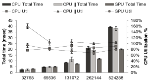
Figure 3: Results of Case Study 1.

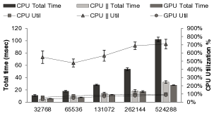
Figure 4: Results of Case Study 2.

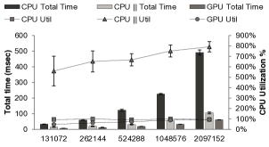
Figure 5: Results of Case Study 3.

  Although the parallel CPU implementation provides reasonable speedup, and the single-core CPU implementation imposes low CPU utilization overhead, the GPU implementation manages to achieve both simultaneously.

6 Related Work

Runtime verification of parametric properties has been studied by Rosu et al [11, 12, 15]. In this line of work, it is possible to build a runtime monitor parameterized by objects in a Java program. The work by Chen and Rosu [8] presents a method of monitoring parametric properties in which a trace is divided into slices, such that each monitor operates on its slice. This resembles our method of identifying trace subsequences and how they are processed by submonitors. However, parametric monitoring does not provide a formalization of applying existential and numerically constrained quantifiers over objects.

Bauer et al. [5] present a formalization of a variant of first order logic combined with LTL. This work is related to our work in that it instantiates monitors at run time according to valuations, and defines quantification over a finite subset of the quantified domain, normally with that subset being defined by the trace. Our work extends this notion with numerical constraints over quantifiers, as well as a parallel algorithm for monitoring such properties.

The work by Leucker et al. presents a generic approach for monitoring modulo theories [9]. This work provides a more expressive specification language. Our work enforces a canonical syntax which is not required in [9], resulting in more expressiveness. However, the monitoring solution provided requires SMT solving at run time. This may induce substantial overhead as opposed to the lightweight parallel algorithm presented in this paper, especially since it is designed to allow offloading the workload on GPU. SMT solving also runs the risk of undecidability, which is not clear whether it is accounted for or not. Ltl${}_{4}-$C is based on six-valued semantics, extending Ltl₄ by two truth values: ${\top_{c}}$ and ${\bot_{c}}$. These truth values are added to support quantifiers and their numerical constraints. This six-valued semantics provides a more accurate assessment of the satisfaction of the property based on finite traces as opposed to the three-valued semantics in [9]. Finally, although Ltl${}_{4}-$C does not support the expressiveness of full first-order logic, numerical constraints add a flavor of second-order logic increasing its expressiveness in the domain of properties where some percentage or count of satisfied instances needs to be enforced.

The work in [1] presents a method of using MapReduce to evaluate LTL properties. The algorithm is capable of processing arbitrary fragments of the trace in parallel. Similarly, the work in [2] presents a MapReduce method for offline verification of LTL properties with first-order quantifiers. Our work uses a similar approach in leveraging MapReduce, yet also adds the expressiveness of counting semantics with numerical constraints. Also, our approach supports both offline and online monitoring by introducing six-valued semantics, which are capable of reasoning about the satisfaction of a partial trace. This is unclear in [2], since there is no evidence of supporting online monitoring.

Finally, the work in [6] presents two parallel algorithms for verification of propositional Ltl specifications at run time. These algorithms are implemented in the tool RiTHM [16]. This paper enhances the framework in [6, 16] by introducing a significantly more expressive formal specification language along with a parallel runtime verification system.

7 Conclusion

In this paper, we proposed a specification language (Ltl${}_{4}-$C) for runtime verification of properties of types of objects in software and networked systems. Our language is an extension of Ltl that adds counting semantics with numerical constraints. The six truth values of the semantics of Ltl${}_{4}-$C allows system designers to obtain informative verdicts about the status of system properties at run time. We also introduced an efficient and effective parallel algorithm with two implementations on multi-core CPU and GPU technologies. The results of our experiments on three real-world case studies show that runtime monitoring using GPU provides us with the best throughput and CPU utilization, resulting in minimal intervention in the normal operation of the system under inspection.

For future work, we are planning to design a framework for monitoring Ltl${}_{4}-$C properties in distributed systems and cloud services. Another direction is to extend Ltl${}_{4}-$C such that it allows non-canonical strings of quantifiers. Finally, we are currently integrating Ltl${}_{4}-$C in our tool RiTHM [16].

References

- [1] Benjamin Barre, Mathieu Klein, Maxime Soucy-Boivin, Pierre-Antoine Ollivier, and Sylvain Hallé. Mapreduce for parallel trace validation of ltl properties. In Runtime Verification, pages 184–198. Springer, 2013.
- [2] David Basin, Germano Caronni, Sarah Ereth, Matúš Harvan, Felix Klaedtke, and Heiko Mantel. Scalable offline monitoring⋆.
- [3] A. Bauer, M. Leucker, and C. Schallhart. Comparing LTL semantics for runtime verification. Journal of Logic and Computation, 20(3):651–674, 2010.
- [4] A. Bauer, M. Leucker, and C. Schallhart. Comparing LTL Semantics for Runtime Verification. Journal of Logic and Computation, 20(3):651–674, 2010.
- [5] Andreas Bauer, Jan-Christoph Küster, and Gil Vegliach. From propositional to first-order monitoring. In Runtime Verification, pages 59–75. Springer Berlin Heidelberg, 2013.
- [6] S. Berkovich, B. Bonakdarpour, and S. Fischmeister. GPU-based runtime verification. In IEEE International Parallel and Distributed Processing Symposium (IPDPS), pages 1025–1036, 2013.
- [7] Maximiliano Caceres. Syscall proxying-simulating remote execution. Core Security Technologies, 2002.
- [8] Feng Chen and Grigore Roşu. Parametric trace slicing and monitoring. In Tools and Algorithms for the Construction and Analysis of Systems, pages 246–261. Springer, 2009.
- [9] Normann Decker, Martin Leucker, and Daniel Thoma. Monitoring modulo theories.
- [10] Idilio Drago, Marco Mellia, Maurizio M Munafo, Anna Sperotto, Ramin Sadre, and Aiko Pras. Inside dropbox: understanding personal cloud storage services. In Proceedings of the 2012 ACM conference on Internet measurement conference, pages 481–494. ACM, 2012.
- [11] Soha Hussein, Patrick Meredith, and Grigore Roşlu. Security-policy monitoring and enforcement with javamop. In Proceedings of the 7th Workshop on Programming Languages and Analysis for Security, PLAS ’12, pages 3:1–3:11, New York, NY, USA, 2012. ACM.
- [12] Dongyun Jin, P.O. Meredith, Choonghwan Lee, and G. Rosu. Javamop: Efficient parametric runtime monitoring framework. In Software Engineering (ICSE), 2012 34th International Conference on, pages 1427–1430, June 2012.
- [13] Leonid Libkin. Elements of finite model theory. springer, 2004.
- [14] Z. Manna and A. Pnueli. Temporal verification of reactive systems - safety. Springer, 1995.
- [15] Patrick Meredith and Grigore Rosu. Efficient parametric runtime verification with deterministic string rewriting. In Automated Software Engineering (ASE), 2013 IEEE/ACM 28th International Conference on, pages 70–80. IEEE, 2013.
- [16] S. Navabpour, Y. Joshi, C. W. W. Wu, S. Berkovich, R. Medhat, B. Bonakdarpour, and S. Fischmeister. Rithm: a tool for enabling time-triggered runtime verification for c programs. In ACM Symposium on the Foundations of Software Engineering (FSE), pages 603–606, 2013.
- [17] Daniel Ramsbrock, Robin Berthier, and Michel Cukier. Profiling attacker behavior following ssh compromises. In Dependable Systems and Networks, 2007. DSN’07. 37th Annual IEEE/IFIP International Conference on, pages 119–124. IEEE, 2007.
- [18] Feng Wang, Qin Xin, Bo Hong, Scott A Brandt, Ethan L Miller, Darrell DE Long, and Tyce T McLarty. File system workload analysis for large scale scientific computing applications. In Proceedings of the 21st IEEE/12th NASA Goddard Conference on Mass Storage Systems and Technologies, pages 139–152, 2004.
- [19] Michael Zink, Kyoungwon Suh, Yu Gu, and Jim Kurose. Watch global, cache local: Youtube network traffic at a campus network: measurements and implications. In Electronic Imaging 2008, pages 681805–681805. International Society for Optics and Photonics, 2008.