Partial Identification of Distributional Parameters
in Triangular Systems

Abstract

I study partial identification of distributional parameters in triangular systems. The model consists of a nonparametric outcome equation and a selection equation. This allows for general unobserved heterogeneity in potential outcomes and selection on unobservables. The distributional parameters considered in this paper are the marginal distributions of potential outcomes, their joint distribution, and the distribution of treatment effects. I explore different types of plausible restrictions to tighten existing bounds on these parameters. The restrictions include stochastic dominance, quadrant dependence between unobservables, and monotonicity between potential outcomes. My identification applies to the whole population without a full support condition on instrumental variables and does not rely on rank similarity. I also provide numerical examples to illustrate identifying power of the restrictions.
Keywords: Partial Identification, Triangular Systems, Stochastic Monotonicity, Monotone Treatment Response, Quadrant Dependence
JEL Classifications: C14, C21, C61, C81.

1 Introduction

In this paper, I consider partial identification of distributional parameters in triangular systems as follows:

$$Y = m\left(D,\varepsilon_{D}\right)\text{,}$$

$$D = \boldsymbol{1}\left[p\left(Z\right)\geq U\right].$$

Here $Y$ denotes a continuous observed outcome, $D$ a binary selection indicator, $Z$ instrumental variables (IV), $\varepsilon_{D}$ a scalar unobservable, and $U$ a scalar unobservable. Let $Y_{0}$ and $Y_{1}$ denote the potential outcomes without and with some treatment, respectively, with $Y_{d}=m\left(d,\varepsilon_{d}\right)$ for $d\in\left\{0,1\right\}$. Note that I suppress covariates included in the outcome equation and the selection equation to keep the notation manageable. The analysis readily extends to accoount for conditioning on these covariates. The distributional parameters that I am interested in are the marginal distributions of $Y_{0}$ and $Y_{1}$, their joint distribution, and the distribution of treatment effects (DTE) $P\left(\Delta\leq\delta\right)$ with the treatment effect $\Delta=Y_{1}-Y_{0}$ and $\delta\in\mathbb{R}$.

In the context of welfare policy evaluation, various distributional parameters beyond the average effects are often of fundamental interest. First, changes in marginal distributions of potential outcomes induced by policy are one of the main concerns when the impact on total social welfare is calculated by comparing the distributions of potential outcomes. Examples include inequality measures such as the Gini coefficient and the Lorenz curve with and without policy (e.g. B2007), and stochastic dominance tests between the distributions of potential outcomes (e.g. A2002). Second, information on the joint distribution of $Y_{0}$ and $Y_{1}$, and the DTE beyond their marginal distributions is often required to capture individual specific heterogeneity in program evaluation. Examples of such information include the distribution of the outcome with treatment given that the potential outcome without treatment lies in a specific set $P\left(Y_{1}\leq y_{1}|Y_{0}\in\Upsilon_{0}\right)$ for some set $\Upsilon_{0}$ in $\mathbb{R}$, the fraction of the population that benefits from the program $P\left(Y_{1}\geq Y_{0}\right),$ the fraction of the population that has gains or losses in a specific range $P\left(\delta^{L}\leq Y_{1}-Y_{0}\leq\delta^{U}\right)$ for $\left(\delta^{L},\delta^{U}\right)\in$ $\mathbb{R}^{2}$ with $\delta^{L}\leq\delta^{U}$, and the $q$ quantile of the impact distribution $\inf\left\{\delta:F_{\Delta}\left(\delta\right)>q\right\}$.

The triangular system considered in this study consists of an outcome equation and a selection equation. This structure allows for general unobserved heterogeneity in potential outcomes and selection on unobservables. The error term in the outcome equation represents unobserved factors causing heterogeneity in potential outcomes among observationally equivalent individuals. The selection model with a latent index crossing a threshold has been widely used to model selection into programs. In the model, the latent index $p\left(Z\right)-U$ is interpreted as the net expected utility from participating in the program. V2002 showed that the model is equivalent to the local average treatment effect (LATE) framework developed by IA1994.

In the literature, the identification method has relied on either the full support of IV or rank similarity to consider the $entire$ population. The full support condition requires IV to change the probability of receiving the treatment from zero to one. As discussed in H1990, and IW2009, however, the applicability of the identification results is very limited because such instruments are difficult to find in practice. Rank similarity assumes that the distribution $\varepsilon_{d}$ conditional on $U$ does not depend on $d$ for $d\in\left\{0,1\right\}$. As a relaxed version of rank invariance, it allows for a random variation between ranks with and without treatment. However, rank similarity is invalid when individuals select treatment status based on their potential outcomes, as in the Roy model.

The literature on identification in triangular systems has stressed marginal distributions more than the joint distribution or the DTE. H1990 point-identified marginal distributions relying on the full support condition. CH2005 showed that the marginal distributions are point-identified for the entire population under rank similarity. Without these conditions, most of the literature has focused on local identification for compliers, to circumvent complications in considering the whole population. IR1997, and A2002 showed that under LATE assumptions presented by IA1994, marginal distributions of potential outcomes are point-identified for compliers who change their selection in a certain direction according to the change in the value of IV. K2009 contrasts with other work in the sense that his identification is for the $entire$ population without relying on the full support of IV and rank similarity. He obtained the identification region for the marginal distributions under IV conditions. The joint distribution and the DTE have not been investigated in these studies.

The literature on identification of the joint distribution and the DTE is relatively small. FW2010 established sharp bounds on the joint distribution and the DTE in semiparametric triangular systems using Fréchet-Hoeffding bounds and Makarov bounds, respectively. Their identification is for the entire population under the full support of IV. Also, GH2012 point-identified the DTE based on a random coefficients specification for the selection equation. To do this, they also relied on the full support of the IV. P2013 studied identification of the joint distribution and the DTE in the extended Roy model, a particular case of triangular systems. Although he point-identified the joint distribution and the DTE by taking advantage of the particular structure of the extended Roy model, his identification only applies to the group of compliers. HSC1997, CHH2003, and Aakvik et al. (2005) considered factor structures in outcome unobservables and assumed the presence of additional proxy variables to identify the joint distribution. HM2014 considered Roy models with a binary outcome variable. They derived sharp bounds on the marginal distributions and the joint distribution of the potential outcomes. Although they did not assume the full support of IV and rank similarity, for the joint distribution bounds they focused on a one-factor structure, as proposed in AHV2005.

The main contribution of this paper is to partially identify the joint distribution and the DTE as well as marginal distributions for the entire population without the full support condition of IV and rank similarity. To avoid strong assumptions and impose plausible information on the model, I consider weak restrictions on dependence between unobservables and between potential outcomes. First, I obtain sharp bounds on the distributional parameters for the worst case, which only assumes the latent index model of V2002. Next, I explore three different types of restrictions to tighten the worst bounds and investigate how each restriction contributes to improving the identification regions of these parameters.

The first restriction that I consider is negative stochastic monotonicity (NSM) between $\varepsilon_{d}$ and $U$ for $d\in\left\{0,1\right\}$. NSM means that $\varepsilon_{d}$ increases as U increases for $d\in\left\{0,1\right\}$. This assumption has been adopted in the literature including JPX2011 for its plausibility in practice. The role of NSM in my paper is different from theirs: I use this condition to bound the counterfactual marginal distributions for the whole population, while they use this condition to identify a particular structure in the outcome equation for individuals who change their selection by variation in IV. Another type of restriction that I discuss is conditional positive quadrant dependence (CPQD) for the dependence between $\varepsilon_{0}$ and $\varepsilon_{1}$ conditional on $U$. CPQD means that $\varepsilon_{0}$ and $\varepsilon_{1}$ are positively dependent conditionally on $U$. Finally, I consider monotone treatment response (MTR) $P\left(Y_{1}\geq Y_{0}\right)=1$, which assumes that each individual benefits from the treatment. Unlike other two restrictions, MTR restricts the support of potential outcomes.

Interesting conclusions emerge from the results of this paper. First, NSM has identifying power on the marginal distributions only. CPQD improves the bounds on the joint distribution only. On the other hand, MTR yields substantially tighter identification regions for all three distributional parameters.

In the next section, I give a formal description of my problem, define the parameters of interest, and discuss assumptions considered for the identification. In Section 3, I establish sharp bounds on the distributional parameters. Section 4 discusses testable implications and considers bounds when some of the restrictions are jointly imposed. Section 5 provides numerical examples to illustrate the identifying power of each restriction and Section 6 concludes. Technical proofs are collected in Appendix.

2 Basic Model and Assumptions

2.1 Model

Consider the triangular system:

$$Y = m\left(D,\varepsilon_{D}\right),$$ (1)

$$D = \boldsymbol{1}\left[p\left(Z\right)\geq U\right],$$

where $Y$ is an observed scalar outcome, $D$ is a binary indicator for treatment participation, $\varepsilon_{D}$ is a scalar unobservable in the outcome equation, and $U$ is a scalar unobservable in a selection equation. Since $Y$ is an realized outcome as a result of selection $D,$ $Y$ can be written as $Y=D\times Y_{1}+(1-D)\times Y_{0}$, where $Y_{0}$ and $Y_{1}$ are potential outcomes for the treatment status $0$ and $1$, respectively. Let $Z$ denote a scalar or vector-valued IV that is excluded from the outcome equation and $\mathcal{Z}$ denote the support of $Z$.  For each $z\in\mathcal{Z}$, let $D_{z}$ be the potential treatment participation when $Z=z$.

Note that I allow the distribution of outcome unobservables to vary with the selection $D$. Also, I do not impose an additively separable structure on the unobservable in the outcome equation. In the selection equation, $p\left(Z\right)-U$ can be interpreted as the net utility from treatment participation. Note that selection on unobservables arises from dependence between $\varepsilon_{D}$ and $U.$

Remark 1

Without loss of generality, I assume that $U\sim Unif\left(0,1\right)$ for normalization. Then $p\left(z\right)=P\left[D=1|Z=z\right]$ is interpreted as a propensity score.

Throughout this study, I impose the following assumptions on the model (1).

M.1 (Monotonicity)

$m\left(d,\varepsilon_{d}\right)$ is strictly increasing in a scalar unobservable $\varepsilon_{d}$ for each $d\in\left\{0,1\right\}.$

M.2 (Continuity)

For $d\in\left\{0,1\right\}$, the distribution function of $\varepsilon_{d}$ is absolutely continuous with respect to the Lebesgue measure on $\mathbb{R}$.

M.3 (Exogeneity)

$Z\perp\!\!\!\perp\left(\varepsilon_{0},\varepsilon_{1},U\right)$.

M.4 (Propensity Score)

The function $p\left(\cdot\right)$ is a nonconstant and continuous function for the continuous element in $Z$.

$M.1$ and $M.2$ ensure the continuous distribution of $Y_{d}$ and invertibility of the function $m\left(d,\varepsilon_{d}\right)$ in the second argument, which is a standard assumption in the literature on nonparametric models with a nonseparable error. $M.3$ is an instrument exogeneity condition. That is, the instrument $Z$ exogenously affects treatment selection and it affects the outcome only through the treatment status. Furthermore, $Z$ does not affect dependence among unobservables $\varepsilon_{0},\varepsilon_{1}$, and $U$. $M.4$ is necessary to ensures sharpness of the bounds. It requires that when some elements of the IV are continuous, the propensity score function $p\left(\cdot\right)$ be continuous for the continuous elements of IV when the discrete elements of IV are held constant. See SV2011 for details.

Remark 2

V2002 showed that under $M.3$, the selection equation in the model (1) is equivalent to the assumptions in the LATE framework developed by IA1994: independence and monotonicity. The LATE independence condition assumes that $Z\perp\!\!\!\perp\left(Y_{0},Y_{1},U\right)$ and that the propensity score $p\left(z\right)$ is a nonconstant function. The LATE monotonicity condition assumes that either $D_{z}\geq D_{z^{\prime}}$ or $D_{z^{\prime}}\geq D_{z}$ with probability one for $\left(z,z^{\prime}\right)\in\mathcal{Z}\times\mathcal{Z}$ with $z\neq z^{\prime}.$

Numerous examples fit into the model (1). I refer to the following three examples throughout the paper.

Example 1

(The effect of job training programs on wages) Let $Y$ be a wage and $D$ be an indicator of enrollment for the program. Let $Z$ be the random assignment for the training service when the program designs randomized offers in the early application process. Note that such a randomized assignment has been widely used as a valid instrument in the LATE framework, which is equivalent to the model (1) considered in this paper.

Example 2

(College premium) Let $Y$ be a wage and $D$ be the college education indicator. The literature including CHV2011 has used the distance to college, local wage, local unemployment rate, and average tuition for public colleges in the county of residence as IV.

Example 3

(The effect of smoking on infant birth weight) Let $Y$ be an infant birth weight and $D$ be a smoking indicator. In the empirical literature, state cigarette taxes, policy interventions including tax hikes, and randomized counselling have been used as IV.

2.2 Objects of Interest and Assumptions

The objects of interest here are the marginal distribution functions of $Y_{0}$ and $Y_{1},$ $F_{0}\left(y_{0}\right)$ and $F_{1}\left(y_{1}\right)$, their joint distribution function $F\left(y_{0},y_{1}\right)$, and the DTE $F_{\Delta}\left(\delta\right)=P\left(Y_{1}-Y_{0}\leq\delta\right)$ for fixed $y_{0}$, $y_{1}$, and $\delta$ in $\mathbb{R}$. I obtain sharp bounds on $F_{0}\left(y_{0}\right),$ $F_{1}\left(y_{1}\right),$ $F\left(y_{0},y_{1}\right),$ and $F_{\Delta}\left(\delta\right)$ under various weak restrictions. First, I derive worst case bounds making use of only $M.1-M.4$ in the model (1). The conditions $M.1-M.4$ are maintained throughout this study. Second, I impose negative stochastic monotonicity (NSM) between each outcome unobservable and the selection unobservable, and show how identification regions improve under the additional restriction. Third, I consider conditional positive quadrant dependence (CPQD) as a restriction between two outcome unobservables $\varepsilon_{0}$ and $\varepsilon_{1}$ conditional on the selection unobservable $U$. I also explore identifying power of this restriction on each parameter, when it is imposed on top of $M.1-M.4$. Lastly, I consider monotonicity between two potential outcomes as a different type of restriction. Henceforth, I call this monotone treatment response (MTR). I derive sharp bounds under MTR in addition to $M.1-M.4$.

First, I present the definition of NSM, CPQD, and MTR. I also illustrate them using a toy model and discuss the underlying intuition with economic examples.

NSM (Negative Stochastic Monotonicity)

Both $\varepsilon_{0}$ and $\varepsilon_{1}$ are first order stochastically nonincreasing in $U.$ That is, $P\left(\varepsilon_{d}\leq e|U=u\right)$ is nondecreasing in $u\in\left(0,1\right)$ for any $e\in\mathbb{R}$ and $d\in\left\{0,1\right\}.$

CPQD (Conditional Positive Quadrant Dependence)

$\varepsilon_{0}$ and $\varepsilon_{1}$ are positively quadrant dependent conditionally on $U.$ That is, for $\left(\varepsilon_{0},\varepsilon_{1}\right)\in\mathbb{R\times R}$ and $u\in\left(0,1\right),$

$$P\left[\varepsilon_{0}\leq e_{0},\varepsilon_{1}\leq e_{1}|U=u\right]\geq P\left[\varepsilon_{0}\leq e_{0}|U=u\right]P\left[\varepsilon_{1}\leq e_{1}|U=u\right].$$

To better understand these restrictions, consider a particular case where $\varepsilon_{0}$ and $\varepsilon_{1}$ have a one-factor structure as follows: for $d\in\left\{0,1\right\}$

$$\varepsilon_{d}=\rho_{d}U+\nu_{d},$$ (2)

where $\left(\nu_{0},\nu_{1}\right)\perp\!\!\!\perp U.$ Here$\ U$ is the unobservable in the selection equation, while $\nu_{0}$ and $\nu_{1}$ represent treatment specific heterogeneity.

In this setting, NSM requires that $\rho_{0}$ and $\rho_{1}$ be nonpositive. Note that the direction of the sign of the monotonicity is not crucial because my identification strategy can be applied to negative stochastic monotonicity. Intuitively, NSM implies that as the level of $U$ increases, both $\varepsilon_{0}$ and $\varepsilon_{1}$ decrease or stay constant. This condition is plausible in many empirical applications. In job training programs, individuals with higher motivation for the training program (lower $U$) are more likely to invest effort in their work (higher $\varepsilon_{0}$ and $\varepsilon_{1}$) than others with lower motivation (higher $U$). In the example of the college premium, a lower reservation utility (lower $U$) for college education $\left(D=1\right)$ is more likely to go with a higher level of unobserved abilities $($higher $\varepsilon_{0}$ and $\varepsilon_{1})$. Regarding the effect of smoking on infant birth weight, NSM suggests that controlling for observed characteristics, individuals with a lower desire (lower $U$) for smoking ($D=0$) are more likely to have a healthier lifestyle $($higher $\varepsilon_{1}$ and $\varepsilon_{0})$ than those with a higher desire (higher $U$).

CPQD excludes any negative dependence between $\nu_{0}$ and $\nu_{1}$ in the example (2). Before discussing implications of CPQD, I present the concept of quadrant dependence. Quadrant dependence between two random variables is defined as follows:

Definition 1

(Positive (Negative) Quadrant Dependence, L1966) Let $X$ and $Y$ be random variables. $X$ and $Y$ are positively (negatively) quadrant dependent if for any $(x,y)\in\mathbb{R}^{2}$,

$$P\left[X\leq x,Y\leq x\right]\geq\left(\leq\right)P\left[X\leq x\right]P\left[Y\leq x\right].$$

or equivalently,

$$P\left[X>x,Y>x\right]\geq\left(\leq\right)P\left[X>x\right]P\left[Y>x\right].$$

Intuitively, $X$ and $Y$ are positively quadrant dependent, if the probability that they are simultaneously small or large is at least as high as it would be if they were independent. Note that quadrant dependence is a very weak dependence measure among a variety of dependence concepts in copula theory.

I impose conditional positive quadrant dependence between $\varepsilon_{0}$ and $\varepsilon_{1}$ given the selection unobservable $U$. In the example (2), CPQD requires that $\nu_{0}$ and $\nu_{1}$ be positively quadrant dependent. Note that CPQD is satisfied even when $\nu_{0}$ and $\nu_{1}$ are independent of each other.

To intuitively understand the implications of CPQD, consider the example (2) for the three examples. For the example of job training programs, suppose that two agents A and B have the same level of motivation for the program and the identical observed characteristics. CPQD implies that if the agent A is likely to earn more than agent B when they both participate in the program, then A is still likely to earn more than B if neither A nor B participates. This is due to the nonnegative correlation between $\nu_{0}$ and $\nu_{1}.$ In the college premium example, the selection unobservable $U$ and another unobservable factor $\nu_{d}$ for $d\in\left\{0,1\right\}$ have been interpreted as an unobserved talent and market uncertainty, respectively, in the literature including Jun et al. (2012). CPQD excludes the case where market uncertainty unobservables $\nu_{0}$ and $\nu_{1}$ are negatively correlated. In the context of the effect of smoking, after controlling for the desire for smoking and all observed characteristics, the smoking (non-smoking) mother whose infant has higher birth weight is more likely to have a heavier infant if she were a non-smoker (smoker). Infant’s weight is affected by mother’s genetic factors $\nu_{d}$ for $d\in\left\{0,1\right\},$ which are independent of her preference for smoking. CPQD requires that mother’s genetic factors in treatment status $0$ and $1,$ $\nu_{0}$ and $\nu_{1}$ are nonnegatively correlated.

MTR (Monotone Treatment Response)

$P\left(Y_{1}\geq Y_{0}\right)=1.$

MTR indicates that every individual benefits from some program or treatment. MTR has been widely adopted in empirical research on evaluation of welfare policy and various treatments including three examples I consider, the effect of funds for low-ability pupils (H2012), the impact of the National School Lunch Program on child health (GKP2011), and various medical treatments (BSV2008, BSV2012).

2.3 Classical Bounds

In this subsection, I present two classical bounds that are applicable to bounds on the joint distribution function and bounds on the DTE when the marginal distributions of $Y_{0}$ and $Y_{1}$ are given. These are referred to frequently throughout the paper.

Suppose that marginal distributions $F_{0}$ and $F_{1}$ are given and no other restriction is imposed on the joint distribution $F$. Sharp bounds on the joint distribution $F$ are given as follows: for $\left(y_{0},y_{1}\right)\in\mathbb{R}\times\mathbb{R},$

$$\max\left\{F_{0}\left(y_{0}\right)+F_{1}\left(y_{1}\right)-1,0\right\}\leq F\left(y_{0},y_{1}\right)\leq\min\left\{F_{0}\left(y_{0}\right),F_{1}\left(y_{1}\right)\right\}.$$

These bounds are referred to as Fréchet-Hoeffding bounds. The lower bound is achieved when $Y_{0}$ and $Y_{1}$ are perfectly negatively dependent, while the upper bound is achieved when they are perfectly positively dependent.

Next, let

$$F_{\Delta}^{L}\left(\delta\right) = \sup_{y}\max\left(F_{1}\left(y\right)-F_{0}\left(y-\delta\right),0\right),$$

$$F_{\Delta}^{U}\left(\delta\right) = 1+\inf_{y}\min\left(F_{1}\left(y\right)-F_{0}\left(y-\delta\right),0\right).$$

Then for the DTE $F_{\Delta}\left(\delta\right)=P\left(\Delta\leq\delta\right)=P\left(Y_{1}-Y_{0}\leq\delta\right),$

$$F_{\Delta}^{L}\left(\delta\right)\leq F_{\Delta}\left(\delta\right)\leq F_{\Delta}^{U}\left(\delta\right),$$

and both $F_{\Delta}^{L}\left(\delta\right)$ and $F_{\Delta}^{U}\left(\delta\right)$ are sharp. These bounds are referred to as Makarov bounds.

3 Sharp Bounds

This section establishes sharp bounds on the marginal distributions of $Y_{0}$ and $Y_{1}$, the joint distribution and the DTE. I start with the worst case bounds which are established under $M.1-M.4$ for model (1). I then obtain bounds under NSM and $M.1-M.4$, bounds under CPQD and $M.1-M.4,$ and finally those under MTR in addition to $M.1-M.4$. To compress long notation, henceforth I refer to $P\left(Y\leq y|D=d,Z=z\right)$, $P\left(Y_{d}\leq y|D=1-d,Z=z\right)$, $P\left(Y\leq y,D=d|Z=z\right),$  and $P\left(Y_{d}\leq y,D=1-d|Z=z\right)$ as $P\left(y|d,z\right)$, $P_{d}\left(y|1-d,z\right),$ $P\left(y,d|z\right)$, and $P_{d}\left(y,1-d|z\right),$ respectively, for $d\in\left\{0,1\right\}$, $y\in\mathbb{R}$, and $z\in\mathcal{Z}$.

3.1 Worst Case Bounds

BGIM2007 obtained sharp bounds on marginal distributions of $Y_{0}$ and $Y_{1}$ under $M.1-M.4.$ I take their approach to bounding the marginal distributions. Given $M.3$, marginal distributions of $Y_{0}$ and $Y_{1}$ can be written as follows: for each $z\in\mathcal{Z}$ and any $y\in\mathbb{R}$,

$$F_{1}\left(y\right) =P\left(Y_{1}\leq y|Z=z\right)$$ (3)

$$=P\left(y,1|z\right)+P_{1}\left(y,0|z\right).$$

While the probability $P\left(y,1|z\right)$ is observed, the counterfactual probability $P_{1}\left(y,0|z\right)$ is never observed. Let $\overline{p}=\underset{z\in\mathcal{Z}}{\sup}p\left(z\right),$ $\underline{p}=\underset{z\in\mathcal{Z}}{\inf}p\left(z\right)$. Note that $\overline{p}$ and $\underline{p}$ are well defined under $M.4$.

For $z\in\mathcal{Z}$ such that $p\left(z\right)<\overline{p},$ the counterfactual probability $P_{1}\left(y,0|z\right)$ can be decomposed as follows:

$$P_{1}\left(y,0|z\right)$$ (4)

$$=P\left(Y_{1}\leq y,p\left(z\right)<U|z\right)$$

$$=P\left(Y_{1}\leq y,p\left(z\right)<U\right)$$

$$=P\left(Y_{1}\leq y,p\left(z\right)<U\leq\overline{p}\right)+P\left(Y_{1}\leq y,\overline{p}<U\right),$$

The second equality follows from $M.3$.

Note that $P\left(Y_{1}\leq y,p\left(z\right)<U\leq\overline{p}\right)$ is point-identified as follows:

$$P\left(Y_{1}\leq y,p\left(z\right)<U\leq\overline{p}\right) =P\left(Y_{1}\leq y,U\leq\overline{p}\right)-P\left(Y_{1}\leq y,U\leq p\left(z\right)\right)$$

$$=\underset{p\left(z\right)\rightarrow\overline{p}}{\lim}P\left(y|1,z\right)\overline{p}-P\left(y|1,z\right)p\left(z\right).$$

However, $P\left(Y_{1}\leq y,\overline{p}<U\right)$ is never observed. Note that for

$$P\left(Y_{1}\leq y,\overline{p}<U\right)=\underset{p\left(z\right)\rightarrow\overline{p}}{\lim}P_{1}\left(y|0,z\right)\left(1-\overline{p}\right),$$

$\underset{p\left(z\right)\rightarrow\overline{p}}{\lim}P_{1}\left(y|0,z\right)$ can be any value between $0$ and $1$. Therefore, I can derive bounds on $P\left(Y_{1}\leq y,\overline{p}<U\right)$ by plugging $0$ and $1$ into the counterfactual distribution $P\left(y|0,\overline{z}\right)$. Similarly, the other counterfactual probability $P_{0}\left(y,1|z\right)$ can be partially identified.

Lemma 1 (BGIM2007)

Under $M.1-M.4$, for any $z\in\mathcal{Z}$, $P_{0}\left(y,1|z\right)$ and $P_{1}\left(y,0|z\right)$ are bounded as follows:

$$P_{0}\left(y,1|z\right) \in\left[L_{01}^{wst}\left(y,z\right),U_{01}^{wst}\left(y,z\right)\right],$$

$$P_{1}\left(y,0|z\right) \in\left[L_{10}^{wst}\left(y,z\right),U_{10}^{wst}\left(y,z\right)\right],$$

where

$$L_{01}^{wst}\left(y,z\right) =\underset{p\left(z\right)\rightarrow\underline{p}}{\lim}P\left(y|0,z\right)\left(1-\underline{p}\right)-P\left(y|0,z\right)\left(1-p\left(z\right)\right),$$

$$U_{01}^{wst}\left(y,z\right) =\underset{p\left(z\right)\rightarrow\underline{p}}{\lim}P\left(y|0,z\right)\left(1-\underline{p}\right)-P\left(y|0,z\right)\left(1-p\left(z\right)\right)+\underline{p},$$

$$L_{10}^{wst}\left(y,z\right) =\underset{p\left(z\right)\rightarrow\overline{p}}{\lim}P\left(y|1,z\right)\overline{p}-P\left(y|1,z\right)p\left(z\right),$$

$$U_{10}^{wst}\left(y,z\right) =\underset{p\left(z\right)\rightarrow\overline{p}}{\lim}P\left(y|1,z\right)\overline{p}-P\left(y|1,z\right)p\left(z\right)+1-\overline{p},$$

and these bounds are sharp.

Proof. The proof is in Appendix.   

Remark 3

If $\underline{p}=0,$ then $P_{0}\left(y,1|z\right)$ is point-identified as $L_{01}^{wst}\left(y,z\right)=U_{01}^{wst}\left(y,z\right).$ On the other hand, if $\overline{p}=1,$ then $P_{1}\left(y,0|z\right)$ is point-identified as $L_{10}^{wst}\left(y,z\right)=U_{10}^{wst}\left(y,z\right).$ Therefore, when the instruments shift the propensity score from $0$ to $1$, both counterfactual probabilities are point-identified, and thus both marginal distributions of potential outcomes are point-identified. This full support condition implies that treatment participation is completely determined by instruments in the limits, and unobservables do not exert any influence on treatment selection in the limits of the propensity score. Therefore, the distributions of potential outcomes are point-identified as they are point-identified in the absence of selection on unobservables.

Note that under $M.1-M.4$, the model (1) does not impose any restriction on dependence between $Y_{0}$ and $Y_{1}$. Hence, Fréchet-Hoeffding bounds and Makarov bounds can be employed to establish sharp bounds on the joint distribution and the DTE, respectively. Specifically, for any $z\in\mathcal{Z},$

$$F\left(y_{0},y_{1}\right)$$ (5)

$$=P\left(Y_{0}\leq y_{0},Y_{1}\leq y_{1}|z\right)$$

$$=P\left(Y_{0}\leq y_{0},Y_{1}\leq y_{1}|0,z\right)\left(1-p\left(z\right)\right)+P\left(Y_{0}\leq y_{0},Y_{1}\leq y_{1}|1,z\right)p\left(z\right).$$

The first equality follows from $M.3$. Now Fréchet-Hoeffding bounds can be established on $P\left(Y_{0}\leq y_{0},Y_{1}\leq y_{1}|0,z\right)$ and $P\left(Y_{0}\leq y_{0},Y_{1}\leq y_{1}|1,z\right)$ based on point-identified $P\left(y_{0}|0,z\right)$ and partially identified $P_{1}\left(y_{1}|0,z\right),$ and partially identified $P_{0}\left(y_{0}|1,z\right)$ and point-identified $P\left(y_{1}|1,z\right),$ respectively.

Note that when marginal distributions are partially identified, sharp bounds on the joint distribution are obtained by taking the union of Fréchet-Hoeffding bounds over all possible pairs of marginal distributions. Similarly, the DTE can be written as

$$P\left(Y_{1}-Y_{0}\leq\delta\right)$$

$$=P\left(Y_{1}-Y_{0}\leq\delta|z\right)$$

$$=P\left(Y_{1}-Y_{0}\leq\delta|0,z\right)\left(1-p\left(z\right)\right)+P\left(Y_{1}-Y_{0}\leq\delta|1,z\right)p\left(z\right),$$

and Makarov bounds can be applied to $P\left(Y_{1}-Y_{0}\leq\delta|0,z\right)$ and $P\left(Y_{1}-Y_{0}\leq\delta|1,z\right)$ based on point-identified $P\left(y_{0}|0,z\right)$ and partially identified $P_{1}\left(y_{1}|0,z\right),$ and partially identified $P_{0}\left(y_{0}|1,z\right)$ and point-identified $P\left(y_{1}|1,z\right),$ respectively.

The specific forms of sharp bounds on marginal distributions of $Y_{0}$ and $Y_{1},$ their joint distribution, and the DTE under $M.1-M.4$ are provided in Theorem 1 in Appendix.

3.2 Negative Stochastic Monotonicity

In this subsection, I additionally impose NSM on dependence between $\varepsilon_{0}$ and $U$ and between $\varepsilon_{1}$ and $U$. I show that NSM has additional identifying power for marginal distributions, but not on the joint distribution nor on the DTE.

First, I use NSM to tighten the bounds on counterfactual probabilities $P_{1}\left(y,0|z\right)$ and $P_{0}\left(y,1|z\right)$. Consider a counterfactual distribution $P_{1}\left(y|0,z\right)=P\left(\varepsilon_{1}\leq m^{-1}\left(1,y\right)|p\left(z\right)<U\right)$. If $p\left(z\right)<\overline{p},$ under NSM, for any $\widehat{p}\left(z\right)\in(p\left(z\right),1],$

$$P\left\{\varepsilon_{1}\leq m^{-1}\left(1,y\right)|p\left(z\right)<U\right\}\geq P\left\{\varepsilon_{1}\leq m^{-1}\left(1,y\right)|p\left(z\right)<U\leq\widehat{p}\left(z\right)\right\}.$$

Since $P\left\{\varepsilon_{1}\leq m^{-1}\left(1,y\right)|p\left(z\right)<U\leq\widehat{p}\left(z\right)\right\}$ is nondecreasing in $\widehat{p}\left(z\right)$ by NSM, for $z\in\mathcal{Z}$ $\setminus p^{-1}\left(\overline{p}\right),$ the highest possible observable lower bound is obtained when $\widehat{p}\left(z\right)=\overline{p}$. Therefore by NSM, for any $z\in\mathcal{Z}\setminus p^{-1}\left(\overline{p}\right),$ NSM implies

$$P_{1}\left(y|0,z\right)$$

$$=P\left(\varepsilon_{1}\leq m^{-1}\left(1,y\right)|p\left(z\right)<U\right)$$

$$\geq P\left(\varepsilon_{1}\leq m^{-1}\left(1,y\right)|p\left(z\right)<U\leq\overline{p}\right)$$

$$=\frac{P\left(\varepsilon_{1}\leq m^{-1}\left(1,y\right),U\leq\overline{p}\right)-P\left(\varepsilon_{1}\leq m^{-1}\left(1,y\right),U\leq p\left(z\right)\right)}{\overline{p}-p\left(z\right)}.$$

Obviously, $P\left(\varepsilon_{1}\leq m^{-1}\left(1,y\right),U\leq\overline{p}\right)$ and $P\left(\varepsilon_{1}\leq m^{-1}\left(1,y\right),U\leq p\left(z\right)\right)$ are point-identified as $\underset{p\left(z\right)\rightarrow\overline{p}}{\lim}P\left(y,1|z\right)$ and $P\left(y,1|z\right)$ for any $z\in\mathcal{Z}.$

Similarly, $P_{0}\left(y|1,z\right)=P\left(\varepsilon_{0}\leq m^{-1}\left(0,y\right)|U\leq p\left(z\right)\right)$ and by NSM, for any $z\in\mathcal{Z}\setminus p^{-1}\left(\underline{p}\right)$

$$P\left(\varepsilon_{0}\leq m^{-1}\left(0,y\right)|U\leq p\left(z\right)\right)$$

$$\leq P\left(\varepsilon_{0}\leq m^{-1}\left(0,y\right)|\underline{p}<U\leq p\left(z\right)\right)$$

$$=\frac{P\left(\varepsilon_{0}\leq m^{-1}\left(0,y\right),\underline{p}<U\right)-P\left\{\varepsilon_{0}\leq m^{-1}\left(0,y\right),p\left(z\right)<U\right\}}{p\left(z\right)-\underline{p}}.$$

Also, $P\left(\varepsilon_{0}\leq m^{-1}\left(0,y\right),\underline{p}<U\right)$ and $P\left(\varepsilon_{0}\leq m^{-1}\left(0,y\right),p\left(z\right)<U\right)$ are point-identified as $\underset{p\left(z\right)\rightarrow\underline{p}}{\lim}P\left(y,0|z\right)$ and $P\left(y,0|z\right)$, respectively, for any $z\in\mathcal{Z}.$ These bounds are tighter than bounds obtained without NSM.

On the other hand, NSM has no additional identifying power on the upper bound on $P_{1}\left(y|0,z\right)$ and the lower bound on $P_{0}\left(y|1,z\right),$ which means that these bounds under NSM are identical to those obtained without NSM.

Lemma 2

Under $M.1-M.4$ and NSM, $P_{0}\left(y,1|z\right)$ and $P_{1}\left(y,0|z\right)$ are bounded as follows:

$$P_{0}\left(y,1|z\right) \in\left[L_{01}^{wst}\left(y,z\right),U_{01}^{sm}\left(y,z\right)\right],$$

$$P_{1}\left(y,0|z\right) \in\left[L_{10}^{wst}\left(y,z\right),U_{10}^{sm}\left(y,z\right)\right],$$

where

$$L_{10}^{sm}\left(y,z\right) =\left\{\begin{tabular}[c]{ll}$\left(\frac{\underset{p\left(z\right)\rightarrow\underline{p}}{\lim}P\left(y,1|z\right)-P\left(y,1|z\right)}{\overline{p}-p\left(z\right)}\right)\left(1-p\left(z\right)\right),$&for any $z\in\mathcal{Z}\setminus p^{-1}\left(\overline{p}\right)$,\\ $0,$&for $z\in p^{-1}\left(\overline{p}\right),$\end{tabular}\ \ \right.,$$

$$U_{01}^{sm}\left(y,z\right) =\left\{\begin{tabular}[c]{ll}$\left(\frac{P\left(y,0|z\right)-\underset{p\left(z\right)\rightarrow\underline{p}}{\lim}P\left(y,0|z\right)}{p\left(z\right)-\underline{p}}\right)p\left(z\right),$&for any $z\in\mathcal{Z}\setminus p^{-1}\left(\underline{p}\right),$\\ $p\left(z\right),$&for $z\in p^{-1}\left(\underline{p}\right),$\end{tabular}\ \ \right.,$$

and these bounds are sharp.

Now, sharp bounds on marginal distributions of $Y_{0}$ and $Y_{1}$ are obtained by plugging the results in Lemma 2 into the counterfactual probabilities.

Note that under NSM, sharp bounds on the joint distribution and sharp bounds on the DTE are still obtained from Fréchet-Hoeffding bounds and Makarov bounds. To illustrate this, consider the case where $\rho_{0}=\rho_{1}=0$ in the example (2). This case satisfies NSM and NSM does not impose any restriction on the dependence between $\nu_{0}$ and $\nu_{1}$. Therefore, sharp bounds on the joint distribution and the DTE are obtained by the same token as in Subsection 3.1.

The specific forms of sharp bounds on marginal distributions of $Y_{0}$ and $Y_{1},$ their joint distribution, and the DTE under $M.1-M.4$ and NSM are provided in Corollary 1 in Appendix.

3.3 Conditional Positive Quadrant Dependence

Unlike NSM, CPQD has no additional identifying power for the joint distribution and the DTE. In this subsection, I impose weak positive dependence between $\varepsilon_{0}$ and $\varepsilon_{1}$ conditional on $U$ by considering CPQD as follows: for any $\left(e_{0},e_{1}\right)\in\mathbb{R}^{2},$

$$P\left[\varepsilon_{0}\leq e_{0}|u\right]P\left[\varepsilon_{1}\leq e_{1}|u\right]\leq P\left[\varepsilon_{0}\leq e_{0},\varepsilon_{1}\leq e_{1}|u\right].$$ (6)

Recall the example (2): for $d\in\left\{0,1\right\},$

$$\varepsilon_{d}=\rho_{d}U+\nu_{d},$$

where $\left(\nu_{0},\nu_{1}\right)\perp\!\!\!\perp U.$ CPQD requires that $\nu_{0}$ and $\nu_{1}$ be positively quadrant dependent. As a restriction on dependence between $\varepsilon_{0}$ and $\varepsilon_{1}$ conditional on $U,$ CPQD has some information on the joint distribution of $Y_{0}$ and $Y_{1}$, but not marginal distribution of $Y_{d},$ which is identified by the distribution of $\varepsilon_{d}$ conditional on $U$ for $d\in\left\{0,1\right\}.$ Specifically, the lower bound on the conditional joint distribution of $\varepsilon_{0}$ and $\varepsilon_{1}$ given $U$ improves under CPQD as shown in (6). This is due to the nonnegative sign restriction on dependence between $\varepsilon_{0}$ and $\varepsilon_{1}$ given $U$ implied by CPQD. Without CPQD, the sharp lower bound and the upper bound on the conditional joint distribution are achieved when the conditional distributions of $\varepsilon_{0}$ given $U$ and $\varepsilon_{1}$ given $U$ are perfectly negatively dependent and perfectly positively dependent, respectively. Under CPQD, however, the dependence is restricted to range from independence to perfectly positive dependence without any negative dependence. Therefore, the lower bound under CPQD is attained when their conditional dependence is independent.

I show that the lower bound on the unconditional joint distribution can be improved from the improved lower bound on the conditional joint distribution. Chebyshev’s integral inequality is useful for deriving the improved lower bound on the joint distribution of $Y_{0}$ and $Y_{1}$ under CPQD:

Chebyshev’s Integral Inequality

If $f$ and $g:[a,b]\longrightarrow\mathbb{R}$ are two comonotonic functions, then

$$\frac{1}{b-a}\int\limits_{a}^{b}f\left(x\right)g\left(x\right)dx\geq\left[\frac{1}{b-a}\int\limits_{a}^{b}f\left(x\right)dx\right]\left[\frac{1}{b-a}\int\limits_{a}^{b}g\left(x\right)dx\right].$$

To establish bounds on the joint distribution, recall (5). For $e_{0}=m^{-1}\left(0,y_{0}\right)$ and $e_{1}=m^{-1}\left(1,y_{1}\right)$ for $\left(y_{0},y_{1}\right)\in\mathbb{R}\times\mathbb{R},$

$$P\left(Y_{0}\leq y_{0},Y_{1}\leq y_{1}|0,z\right)$$

$$=P\left(\varepsilon_{0}\leq e_{0},\varepsilon_{1}\leq e_{1}|U>p\left(z\right)\right).$$

Now I require the additional assumption:

M.5

The propensity score $p(z)$ is bounded away from $0$ and $1$.

Under $M.5$, Chebyshev’s integral inequality yields the lower bound as follows:

$$P\left(\varepsilon_{0}\leq e_{0},\varepsilon_{1}\leq e_{1}|U>p\left(z\right)\right)$$ (7)

$$=\frac{1}{1-p\left(z\right)}\int\limits_{p\left(z\right)}^{1}P\left[\varepsilon_{0}\leq e_{0},\varepsilon_{1}\leq e_{1}|u\right]du$$

$$\geq\frac{1}{1-p\left(z\right)}\int\limits_{p\left(z\right)}^{1}P\left[\varepsilon_{0}\leq e_{0}|u\right]P\left[\varepsilon_{1}\leq e_{1}|u\right]du$$

$$\geq\left(\frac{1}{1-p\left(z\right)}\right)^{2}\int\limits_{p\left(z\right)}^{1}P\left[\varepsilon_{0}\leq e_{0}|u\right]du\int\limits_{p\left(z\right)}^{1}P\left[\varepsilon_{1}\leq e_{1}|u\right]du.$$

The inequality in the third line of (7) follows from CPQD and the inequality in the fourth line of (7) is due to Chebyshev’s integral inequality. Consequently, I obtain the following:

$$P\left(Y\leq y_{0},Y_{1}\leq y_{1}|0,z\right) \geq P\left(y_{0}|0,z\right)P_{1}\left(y_{1}|0,z\right)$$ (8)

$$\geq\frac{P\left(y_{0}|0,z\right)L_{10}^{wst}\left(y_{1},z\right)}{1-p\left(z\right)}.$$

Similarly, the lower bound on $P\left(Y_{0}\leq y_{0},Y\leq y_{1}|1,z\right)$ is obtained as follows:

$$P\left(Y_{0}\leq y_{0},Y\leq y_{1}|1,z\right) \geq P_{0}\left(y_{0}|1,z\right)P\left(y_{1}|1,z\right)$$ (9)

$$\geq\frac{L_{01}^{wst}\left(y_{0},z\right)P\left(y_{1}|1,z\right)}{p\left(z\right)}.$$

Interestingly, the DTE is still bounded by Makarov bounds under CPQD although the lower bound on the joint distribution improves. The rigorous proof is provided in Appendix. Here I discuss the reason intuitively using a graphical illustration. As shown in Figure 1, the DTE is a probability corresponding to the region below the straight line $y_{1}=y_{0}+\delta$ and the Makarov lower bound is obtained from the rectangle $\left\{Y_{0}\geq y-\delta,Y_{1}\leq y\right\}$ below the straight line $Y_{1}=Y_{0}+\delta$ for $y\in\mathbb{R}$ that maximizes the Fréchet-Hoeffding lower bound. Since the Fréchet-Hoeffding lower bound on $P\left(Y_{0}\geq y-\delta,Y_{1}\leq y\right)$ for each $y\in\mathbb{R}$ is achieved when the joint distribution of $Y_{0}$ and $Y_{1}$ attains its upper bound, the improved lower bound on $F\left(y_{0},y_{1}\right)$ does not affect the lower bound on the DTE. Similarly, the Makarov upper bound is obtained from the upper bound on $1-P\left(Y_{0}\leq y^{\prime}-\delta,Y_{1}\geq y^{\prime}\right)$ for $y^{\prime}\in\mathbb{R}$, which is in turn obtained from the Fréchet-Hoeffding lower bound on $P\left(Y_{0}\leq y^{\prime}-\delta,Y_{1}\geq y^{\prime}\right).$ Therefore by the same token, the improved lower bound on $F\left(y_{0},y_{1}\right)$ does not affect the upper bound on the DTE either.

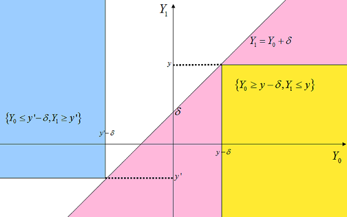
Figure 1: Makarov bounds

The specific forms of sharp bounds on marginal distributions of $Y_{0}$ and $Y_{1},$ their joint distribution, and the DTE under $M.1-M.5$ and CPQD are provided in Theorem 2 in Appendix.

3.4 Monotone Treatment Response

In this subsection, I maintain $M.1-M.4$ on the model (1) and additionally impose MTR, which is written as $P\left(Y_{1}\geq Y_{0}\right)=1$. As illustrated in Figure 2, MTR is a restriction imposed on the support of $(Y_{0},Y_{1})$, while NSM and CPQD directly restrict the sign of dependence between unobservables. I show that MTR has substantial identifying power for the marginal distributions, the joint distribution, and the DTE.

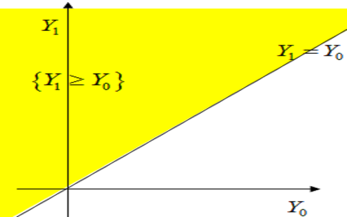
Figure 2: Support under MTR

Start with bounds on marginal distributions. Remember that NSM as well as $M.1-M.4$ has no additional identifying power for the upper bound on $P_{1}\left(y,0|z\right)$ and the lower bound on $P_{0}\left(y,1|z\right)$. Interestingly, MTR improves both the upper bound on $P_{1}\left(y,0|z\right)$ and the lower bound on $P_{0}\left(y,1|z\right).$ On the other hand, unlike NSM, MTR does not have any identifying power on the lower bound on $P_{1}\left(y,0|z\right)$ and the upper bound on $P_{0}\left(y,1|z\right).$ Recall that in (4),

$$P_{1}\left(y,0|z\right)$$

$$=P\left(Y_{1}\leq y,p\left(z\right)<U\leq\overline{p}\right)+P\left(Y_{1}\leq y|\overline{p}<U\right)\left(1-\overline{p}\right).$$

Since MTR implies stochastic dominance of $Y_{1}$ over $Y_{0}$, under MTR,

$$P\left(Y_{1}\leq y|\overline{p}<U\right)\leq P\left(Y_{0}\leq y|\overline{p}<U\right)=\underset{p\left(z\right)\rightarrow\overline{p}}{\lim}P\left(y|0,z\right).$$

Similarly,

$$P\left(Y_{0}\leq y|U\leq\underline{p}\right)\geq P\left(Y_{1}\leq y|U\leq\underline{p}\right)=\underset{p\left(z\right)\rightarrow\underline{p}}{\lim}P\left(y|1,z\right).$$

This shows that MTR tightens the upper bound on $P_{1}\left(y,0|z\right)$ and the lower bound on $P_{0}\left(y,1|z\right)$.

Lemma 3

Under $M.1-M.4$ and MTR, $P_{1}\left(y,0|z\right)$ and $P_{0}\left(y,1|z\right)\$are bounded as follows:

$$P_{1}\left(y,0|z\right) \in\left[L_{10}^{wst}\left(y,z\right),U_{10}^{mtr}\left(y,z\right)\right],$$

$$P_{0}\left(y,1|z\right) \in\left[L_{01}^{mtr}\left(y,z\right),U_{01}^{wst}\left(y,z\right)\right],$$

where

$$L_{01}^{mtr}\left(y,z\right) =\underset{p\left(z\right)\rightarrow\underline{p}}{\lim}P\left(y|0,z\right)\left(1-\underline{p}\right)-P\left(y|0,z\right)\left(1-p\left(z\right)\right)+\underset{p\left(z\right)\rightarrow\underline{p}}{\lim}P\left(y|1,z\right)\underline{p},$$

$$U_{10}^{mtr}\left(y,z\right) =\underset{p\left(z\right)\rightarrow\overline{p}}{\lim}P\left(y|1,z\right)\overline{p}-P\left(y|1,z\right)p\left(z\right)+\underset{p\left(z\right)\rightarrow\overline{p}}{\lim}P\left(y|0,z\right)\left(1-\overline{p}\right),$$

and these bounds are sharp.

From Lemma 3, sharp bounds on marginal distributions of $Y_{0}$ and $Y_{1}$ are improved based on $L_{01}^{mtr}\left(y,z\right)$ and $U_{10}^{mtr}\left(y|z\right)$ under $M.1-M.4$, and MTR as follows:

$$F_{0}^{L}\left(y\right) =\underset{z\in\mathcal{Z}}{\sup}\left[P\left(y|0,z\right)\left(1-p\left(z\right)\right)+L_{01}^{mtr}\left(y,z\right)\right],$$

$$F_{0}^{U}\left(y\right) =\underset{z\in\mathcal{Z}}{\inf}\left[P\left(y|0,z\right)\left(1-p\left(z\right)\right)+U_{01}^{wst}\left(y,z\right)\right],$$

$$F_{1}^{L}\left(y\right) =\underset{z\in\mathcal{Z}}{\sup}\left[P\left(y|1,z\right)p\left(z\right)+L_{10}^{wst}\left(y,z\right)\right],$$

$$F_{1}^{U}\left(y\right) =\underset{z\in\mathcal{Z}}{\inf}\left[P\left(y|1,z\right)p\left(z\right)+U_{10}^{mtr}\left(y,z\right)\right].$$

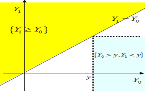
Figure 3: $P\left(Y_{0}>Y_{1}\right)=P\left[\underset{y\in\mathbb{R}}{\cup}\left\{Y_{0}>y,Y_{1}<y\right\}\right]$

Now, I show that MTR also has identifying power for the joint distribution. I will use Lemma 4 to bound the joint distribution under MTR. Henceforth, $x^{+}$ denotes $max\left(x,0\right).$

Lemma 4

(N2006) Suppose that marginal distributions $F_{0}$ and $F_{1}$ are known and that $F\left(a_{0},a_{1}\right)=\theta$ where $\left(a_{0},a_{1}\right)\in\mathbb{R}^{2}$ and $\theta$ satisfies $\max\left(F_{0}\left(a_{0}\right)+F_{1}\left(a_{1}\right)-1,0\right)\leq\theta\leq\min\left(F_{0}\left(a_{0}\right),F_{1}\left(a_{1}\right)\right).$ Then, sharp bounds on the joint distribution $F$ are given as follows:

$$F^{L}\left(y_{0},y_{1}\right)\leq F\left(y_{0},y_{1}\right)\leq F^{U}\left(y_{0},y_{1}\right),$$

where

$$F^{L}\left(y_{0},y_{1}\right) =\max\left\{0,F_{0}\left(a_{0}\right)+F_{1}\left(a_{1}\right)-1,\theta-\left(F_{0}\left(a_{0}\right)-F_{0}\left(y_{0}\right)\right)^{+}-\left(F_{1}\left(a_{1}\right)-F_{1}\left(y_{1}\right)\right)^{+}\right\},$$

$$F^{L}\left(y_{0},y_{1}\right) =\min\left\{F_{0}\left(y_{0}\right),F_{1}\left(y_{1}\right),\theta+\left(F_{0}\left(y_{0}\right)-F_{0}\left(a_{0}\right)\right)^{+}+\left(F_{1}\left(y_{1}\right)-F_{1}\left(a_{1}\right)\right)^{+}\right\}.$$

Suppose that marginal distributions $F_{0}$ and $F_{1}$ are fixed. Lemma 4 shows that sharp bounds on the joint distribution improve when the values of the joint distribution are known at some fixed points. Note that $P\left(Y_{1}\geq Y_{0}\right)=1$ if and only if $F\left(y,y\right)=F_{1}\left(y\right)$ for all $y\in\mathbb{R}.$ As illustrated in Figure 3,

$$P\left(Y_{0}>Y_{1}\right)=P\left[\underset{y\in\mathbb{R}}{\cup}\left\{Y_{0}>y,Y_{1}<y\right\}\right].$$

Therefore,

$\begin{array}[c]{cl}&P\left(Y_{1}\geq Y_{0}\right)=1\\ \Longleftrightarrow&P\left(Y_{0}>Y_{1}\right)=0\\ \Longleftrightarrow&P\left(Y_{0}>y,Y_{1}<y\right)=0\text{ for all }y\in\mathbb{R}\\ \Longleftrightarrow&F\left(y,y\right)=F_{1}\left(y\right),\text{ for all }y\in\mathbb{R}.\end{array}$

Since for each $y\in\mathbb{R}$ the value of $F\left(y,y\right)$ is known from the fixed marginal distribution $F_{1}$ under MTR, sharp bounds on the joint distribution can be derived by taking the intersection of the bounds under the restriction $F\left(y,y\right)=F_{1}\left(y\right)$ over all $y$ $\in\mathbb{R}$. Technical details are presented in Appendix.

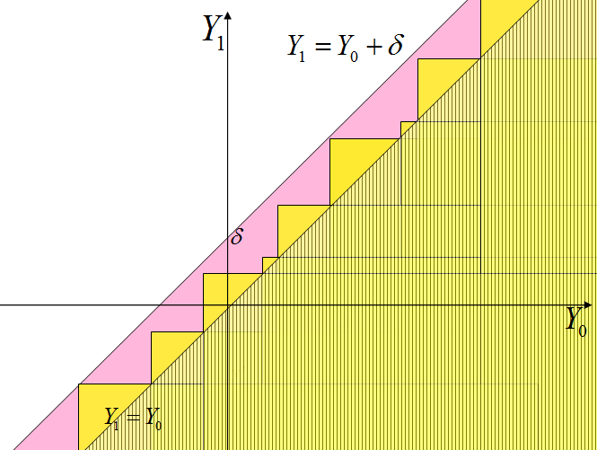
Figure 4: Improved lower bound on the DTE under MTR

In Chapter 1, I obtained sharp bounds on the DTE when marginal distributions are fixed and MTR is imposed. Compared to Figure 1, Figure 4 shows that under MTR the lower bound on the DTE improves by allowing more mass to be added between $Y_{1}=Y_{0}+\delta$ and $Y_{1}=Y_{0}$. Lemma 5 presents sharp bounds on the DTE under MTR and fixed marginals $F_{0}$ an $F_{1}$ as follows:

Lemma 5

(K2014) Under MTR, sharp bounds on the DTE are given as follows: for fixed marginals $F_{0}$ an $F_{1}$ and any $\delta\in\mathbb{R},$

$$F_{\Delta}^{L}\left(\delta\right)\leq F_{\Delta}\left(\delta\right)\leq F_{\Delta}^{U}\left(\delta\right),$$

where

$$F_{\Delta}^{U}\left(\delta\right) =\left\{\begin{array}[c]{cc}1+\underset{y\in\mathbb{R}}{\inf}\left\{\min\left(F_{1}\left(y\right)-F_{0}\left(y-\delta\right)\right),0\right\},&\text{for }\delta\geq 0,\\ 0,&\text{for }\delta<0.\end{array}\right.,$$

$$F_{\Delta}^{L}\left(\delta\right) =\left\{\begin{array}[c]{cc}\underset{\left\{a_{k}\right\}_{k=-\infty}^{\infty}\in\mathcal{A}_{\delta}}{\sup}\sum\limits_{k=-\infty}^{\infty}\max\left\{F_{1}\left(a_{k+1}\right)-F_{0}\left(a_{k}\right),0\right\},&\text{for }\delta\geq 0,\\ 0,&\text{for }\delta<0,\end{array}\right.$$

$$\text{where }\mathcal{A}_{\delta} =\left\{\left\{a_{k}\right\}_{k=-\infty}^{\infty};0\leq a_{k+1}-a_{k}\leq\delta\text{ for every integer }k\right\}.$$

From Lemmas 3, 4, and 5, it is straightforward to derive sharp bounds on the joint distribution and the DTE under $M.1-M.4$ and MTR.

The specific forms of sharp bounds on marginal distributions of $Y_{0}$ and $Y_{1},$ their joint distribution, and the DTE under $M.1-M.4$ and MTR are provided in Theorem 3 in Appendix.

4 Discussion

4.1 Testable Implications

I here show that NSM and MTR yield testable implications.

Note that NSM implies the following: for any $\left(z^{\prime},z\right)\in\mathcal{Z}\times\mathcal{Z}$ such that $p\left(z^{\prime}\right)\geq p\left(z\right),$ and for any $y\in\mathbb{R}$,

$$P\left(\varepsilon_{1}\leq m^{-1}\left(1,y\right)|U\leq p\left(z\right)\right) \leq P\left(\varepsilon_{1}\leq m^{-1}\left(1,y\right)|U\leq p\left(z^{\prime}\right)\right),$$

$$P\left(\varepsilon_{0}\leq m^{-1}\left(0,y\right)|U>p\left(z\right)\right) \leq P\left(\varepsilon_{0}\leq m^{-1}\left(0,y\right)|U>p\left(z^{\prime}\right)\right).$$

This yields the following testable form of functional inequalities:

$$P\left(y|1,z\right) \leq P\left(y|1,z^{\prime}\right),$$ (10)

$$P\left(y|0,z\right) \leq P\left(y|0,z^{\prime}\right).$$

Next, MTR has two testable implications. First, MTR implies stochastic dominance. In our model, marginal distributions are partially identified for the entire population. Therefore, it can be tested by applying econometric techniques for testing stochastic dominance for partially identified marginal distributions as proposed in the literature including Jun et al. (2013). Also, the sharp lower bound on the DTE under MTR can be greater than the upper bound and furthermore the lower bound could be even above 1, when MTR is violated for the true joint distribution of $Y_{0}$ and $Y_{1}$.

4.2 NSM+CPQD and NSM+MTR

In Section 3, I explored the identifying power of NSM, CPQD, and MTR, separately. In this subsection, I briefly discuss how sharp bounds are constructed when some of these conditions are combined. Establishing sharp bounds under NSM and CPQD and sharp bounds under NSM and MTR is straightforward from the results in Subsection 3.2 - Subsection 3.4. First, under NSM and CPQD, bounds on marginal distributions and bounds on the DTE are identical to those under NSM only, since CPQD has no identifying power on the marginal distributions and the DTE. The bounds on the joint distribution under NSM and CPQD can be established by plugging the bounds on the counterfactual probabilities $P_{0}\left(y_{0},1|z\right)$ and $P_{1}\left(y_{1},0|z\right)$ under NSM into the upper bound formula under CPQD as follows:

$$F^{L}\left(y_{0},y_{1}\right) =\underset{z\in\mathcal{Z}}{\sup}\left\{P\left(y_{0}|0,z\right)L_{10}^{sm}\left(y_{1},z\right)+L_{01}^{wst}\left(y_{0},z\right)P\left(y_{1}|1,z\right)\right\},$$

$$F^{U}\left(y_{0},y_{1}\right) =\inf_{z\in\mathcal{Z}}\left[\begin{array}[c]{c}\min\left\{P\left(y_{0}|0,z\right)\left(1-p\left(z\right)\right),U_{10}^{wst}\left(y,z\right)\right\}\\ +\min\left\{U_{01}^{sm}\left(y_{0},z\right),P\left(y_{1}|1,z\right)p\left(z\right)\right\}\end{array}\right].$$

Similarly, the distributional parameters are bounded under NSM and MTR. The specific forms of sharp bounds on marginal distributions of $Y_{0}$ and $Y_{1},$ their joint distribution, and the DTE under $M.1-M.4,$ NSM, and MTR are provided in Theorem 2 in Appendix.

Lastly, marginal distribution bounds under NSM, CPQD, and MTR and marginal distribution bounds under CPQD and MTR are identical to those under NSM and MTR and those under MTR, respectively, since CPQD does not affect bounds on marginal distributions. However, it is not straightforward to construct sharp bounds on the joint distribution and the DTE under these three conditions or under CPQD and MTR, as both CPQD and MTR directly restrict the joint distribution as different types of conditions. To the best of my knowledge, there exist no results on the sharp bounds on the joint distribution and DTE when support restrictions such as MTR are combined with various dependence restriction such as quadrant dependence. This is beyond the scope of this paper.

5 Numerical Examples

This section presents numerical examples to illustrate how bounds on distributional parameters are tightened by the restrictions considered in this paper. The potential outcomes and selection equations are given as follows:

$$Y_{0} =\rho U+\varepsilon,$$

$$Y_{1} =Y_{0}+\eta,$$

$$D\left(Z\right) =1\left(Z\geq U\right),$$

where $\left(U,\varepsilon\right)\sim i.i.d.N\left(0,I_{2}\right)$, $\eta\sim\chi^{2}\left(k\right)$, and $\eta\perp\!\!\!\perp\left(U,\varepsilon\right)$  for a positive integer $k.$

Selection is allowed to be endogenous since the selection unobservable $U$  is dependent on potential outcomes $Y_{0}$ and $Y_{1}$ for $\rho\neq 0$. I consider negative values of $\rho$ to make the specification satisfy NSM discussed in Subsection 3.2. CPQD holds due to the common factor $\varepsilon$ in $Y_{0}$ and $Y_{1}$, which is independent of $U$. Lastly, MTR is obviously satisfied as $P\left(Y_{1}\geq Y_{0}\right)=1$ since $\eta\geq 0$ with probability one. Also, to rule out the full support of the instrument, $Z$ is assumed to be a uniformly distributed random variable on $\left(z,-z\right)$ for $z=2,1.5,1,.5.$

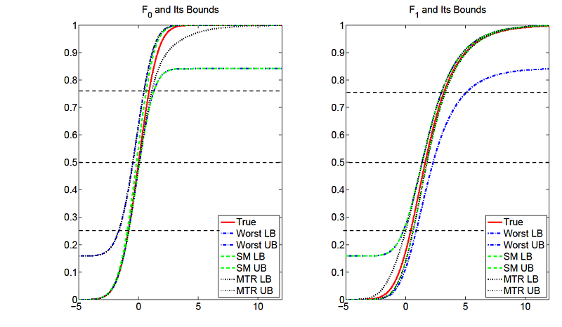
Figure 5: Bounds on the distributions of $Y_{0}$ (left) and $Y_{1}$ (right)

First, for $\rho=-0.75$ and $Z\sim Unif\left(1,-1\right),$ I obtain the sharp bounds on the marginal distributions of potential outcomes $Y_{0}$ and $Y_{1}$ as proposed in Section 3. Figure 5 shows the bounds on each potential outcome distribution as well as the true distribution. Solid curves represent the true marginal distributions of $Y_{0}$ and $Y_{1}$ and dash-dot curves, dotted curves, and dashed curves represent their worst bounds, bounds under NSM, and bounds under MTR, respectively. Remember that bounds on marginal distributions under CPQD are identical to worst bounds. Figure 5 shows that NSM substantially improves the upper bound on $F_{0}$ and the lower bound on $F_{1}$, compared to worst bounds. As shown in Lemma 2, NSM improves the upper bound on $P\left(Y_{0}\leq y,1|z\right)$ and the lower bound on $P\left(Y_{1}\leq y,0|z\right)$ for $y\in\mathbb{R},$ which are used in obtaining the upper bound on $F_{0}$ and the lower bound on $F_{1},$ respectively. On the other hand, MTR improves the lower bound on $F_{0}$ and the upper bound on $F_{1}$.  Note that in contrast to NSM, MTR improves the lower bound on $P\left(Y_{0}\leq y,1|z\right)$ and the upper bound on $P\left(Y_{1}\leq y,0|z\right)$ for all $y\in\mathbb{R},$ which are used in obtaining the lower bound on $F_{0}$ and the upper bound on $F_{1},$ respectively.

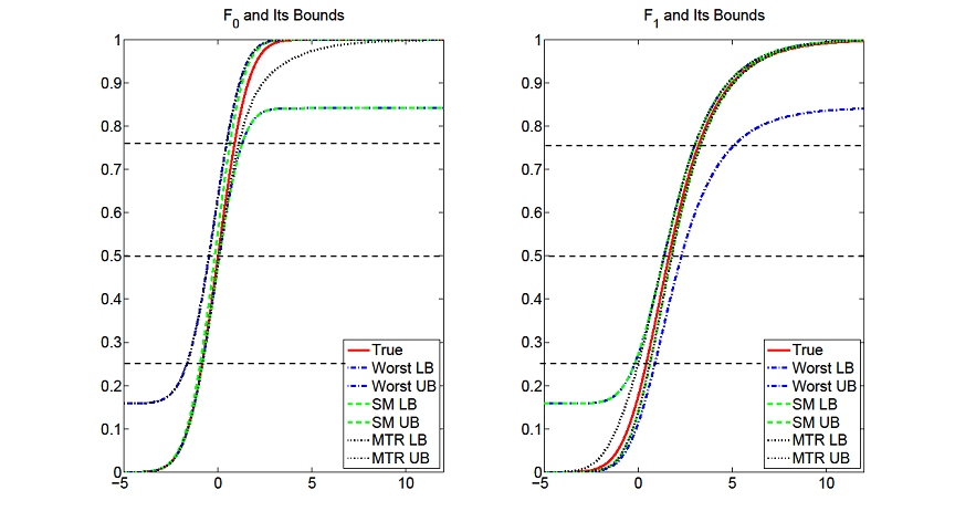
Figure 6: Bounds on the distributions of $Y_{0}$ (left) and $Y_{1}$ (right)

Next, I plotted bounds on marginal distributions when NSM and MTR are jointly imposed. In Figure 6, solid curves represent the true distributions of $Y_{0}$ and $Y_{1},$ and dash-dot curves and dashed curves represent their worst bounds and bounds under NSM and MTR, respectively. Figure 6 shows that if NSM and MTR are jointly considered, both upper and lower bounds improve for both $F_{0}$ and $F_{1}$ as discussed in Section 4. The quantiles of the potential outcomes can be obtained by inverting the bounds on the marginal distributions. The bounds on the quantiles of $Y_{0}$ and $Y_{1}$ are reported in Table 1

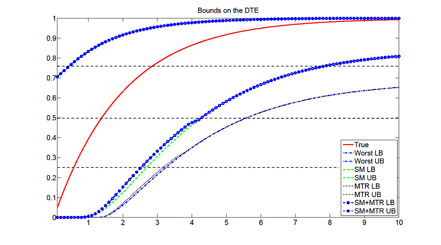
Figure 7: True DTE and bounds on the DTE

Figure 7 shows the true DTE and bounds on the DTE. Solid curve, dash-dot curves, dotted lines, dashed curves, and  dashed curves with circles represent the true DTE, worst DTE bounds, bounds under NSM, bounds under MTR, and bounds under NSM and MTR, respectively. Compared to the worst bounds, the lower bound under NSM notably improves over the entire support of the DTE. Remember that the lower DTE bound improves through the upper bound on $P_{0}\left(y,1|z\right)$ and the lower bound on $P_{1}\left(y,0|z\right),$ both of which are improved by NSM, even though the DTE bounds under NSM still relies on Makarov bounds. On the other hand, although MTR directly improves the lower DTE bound from the Makarov lower bound, the improvement of the lower DTE bound by MTR is not substantial over the whole support. This is because neither the upper bound on $P_{0}\left(y,1|z\right)$ nor the lower bound on $P_{1}\left(y,0|z\right)$ improves, which are the counterfactual components consisting of the lower bound. Also, as discussed in Chapter 1, the sharp lower bound on $F_{\Delta}\left(\delta\right)$ under MTR converges to the Makarov lower bound as $\delta$ increases for sufficiently large values of $\delta.$ On the other hand, the upper bound under NSM does not improve from the worst upper bound as discussed in Subsection 3.2 Although the upper bound improves under MTR through improvement in the lower bound on $P_{0}\left(y,1|z\right)$ and the upper bound on $P_{1}\left(y,0|z\right)$, the improvement in the upper bound under MTR is not remarkable as shown in Figure 7. Also, the quantiles of treatment effects can be obtained by inverting the bounds on the DTE. The bounds on the quantiles of the DTE are reported in Table 1.

Table 2 shows the bounds on the joint distribution under various restrictions considered in this study. Compared to the worst bounds, bounds are tighter under NSM due to the marginal distributions bounds improved by NSM. On the other hand, the upper bound under CQPD does not improve unlike the lower bound. Note that CQPD has no identifying power on marginal distributions, while it improves the lower bound on the joint distribution. However, when CQPD is combined with NSM, the upper bound also improves due to the improved marginal distributions bounds under NSM. The identification region under MTR is tighter than the worst identification region for both the upper bound and the lower bound. Note that the upper bound under MTR is lower than the worst lower bound through the improved lower bound on $P_{0}\left(y,1|z\right)$ and improved upper bound on $P_{1}\left(y,0|z\right)$ by MTR, while it still poses the Makarov upper bound. On the other hand, the lower bound under MTR is higher than the worst lower bound obtained from the Makarov lower bound because of the direct effect of MTR on the lower bound on the joint distribution. Remember that the lower bound on the joint distribution is not affected by the improved components of the bounds on counterfactual probabilities: the improved lower bound on $P_{0}\left(y,1|z\right)$ and improved upper bound on $P_{1}\left(y,0|z\right)$. Lastly, under NSM and MTR both the lower bound and the upper bound improve through counterfactual probabilities $U_{01}^{sm}(y,z)$ and$\ L_{10}^{sm}(y,z)$, respectively which are improved by NSM compared to the bounds under MTR only.

I also obtained sharp bounds on the potential outcomes distributions and the DTE for $z\in\left\{2,1.5,1,.5\right\}$ to see how the support of the instrument affect the identification region. Tables 3, 4, and 5 document the identification regions of $F_{0},$ $F_{1},$ and $F_{\Delta},$ respectively, under NSM and MTR for these different values of $z.$ As expected, as the support of the instrument gets larger, the identification regions of the marginal distributions and the DTE become more informative. Table 5 shows the identification regions of the DTE for different values of $\rho=\left\{-.25,-.5,-.75\right\}$. Since the true DTE does not depend on the value of $\rho,$ one can see from Table 5 how the size of correlation between the outcome heterogeneity and the selection heterogeneity affects the identification region of the DTE for the fixed true DTE. As shown in Table 5, the identification region becomes tighter as $\rho$ approaches $0$. That is, the weaker endogeneity with the smaller absolute value of $\rho$ helps identification of the DTE. This is readily understood from the extreme case. If $\rho=0$ where the treatment selection is independent of potential outcomes $Y_{0}$ and $Y_{1},$ marginal distributions of potential outcomes are exactly identified, which clearly leads to tighter bounds on the DTE.

6 Conclusion

In this paper, I established sharp bounds on marginal distributions of potential outcomes, their joint distribution, and the DTE in triangular systems. To do this, I explored various types of restrictions to tighten the existing bounds including stochastic monotonicity between each outcome unobservable and the selection unobservable, conditional positive quadrant dependence between two outcome unobservables given the selection unobservable, and the monotonicity of the potential outcomes. I did not rely on rank similarity and the full support of IV, and furthermore I avoided strong distributional assumptions including a single factor structure, which contrasts with most of related work. The proposed bounds take the form of intersection bounds and lend themselves to existing inference methods developed in CLR2013.

Table 1: True quantiles and bounds on the quantiles of $Y_{0}$ and $Y_{1}$

$q$		$F_{0}^{-1}\left(q\right)$	$F_{1}^{-1}\left(q\right)$	$F_{\Delta}^{-1}\left(q\right)$
$.25$	True	$-.85$	$.40$	$.48$
	Worst	$[-1.70,-.85]$	$[-.20,.90]$	$[0,3.15]$
	NSM	$[-.95,-.85]$	$[-.20,.60]$	$[0,2.60]$
	MTR	$[-1.70,-.85]$	$[0,.60]$	$[0,3.05]$
	NSM+MTR	$[-.95,-.85]$	$[0,.60]$	$[0,2.40]$
$.5$	True	$0$	$1.65$	$1.30$
	Worst	$[-.45,.05]$	$[0,2.30]$	$[0,5.50]$
	NSM	$[-.15.05]$	$[1.40,1.80]$	$[0,4.20]$
	MTR	$[-.45,.05]$	$[1.40,1.80]$	$[0,5.50]$
	NSM+MTR	$[-.15,.05]$	$[1.40,1.80]$	$[0,4.20]$
$.75$	True	$.85$	$3.15$	$2.70$
	Worst	$[.40,1.20]$	$[2.95,4.95]$	$[.25,\infty)$
	NSM	$[.60,1.20]$	$[2.95,3.30]$	$[.25,7.40]$
	MTR	$[.40,1.05]$	$[2.95,3.30]$	$[.25,\infty)$
	NSM+MTR	$[.60,1.05]$	$[2.95,3.30]$	$[.25,7.40]$

Table 2: True Joint distribution $F\left(y_{0},y_{1}\right)$ and its bounds under various restrictions

$y_{0}\backslash y_{1}$		$-3$	$-1$	$1$	$3$	$5$	$7$	$9$
$-1$	True	$0$	$.03$	$.16$	$.19$	$.20$	$.21$	$.21$
	Worst	$[0,.09]$	$[0,.12]$	$[0,.23]$	$[0,.30]$	$[.03,.34]$	$[.09,.36]$	$[.11,.36]$
	NSM	$[0,.09]$	$[0,.12]$	$[0,.23]$	$[0,.24]$	$[.13,.24]$	$[.18,.24]$	$[.20,.24]$
	CPQD	$[0,.09]$	$[.01,.12]$	$[.06,.23]$	$[.13,.30]$	$[.15,.34]$	$[.16,.36]$	$[.17,.36]$
	NSM+CPQD	$[0,.09]$	$[.01,.12]$	$[.08,.23]$	$[0.16,.24]$	$[.19,.24]$	$[.20,.24]$	$[.21,.24]$
	MTR	$[0,.01]$	$[.03,.12]$	$[.03,.23]$	$[.03,.30]$	$[.03,.34]$	$[.09,.36]$	$[.11,.36]$
	NSM+MTR	$[0,.01]$	$[.03,.12]$	$[.03,.23]$	$[.03.24]$	$[.13,.24]$	$[.18,.24]$	$[.20,.24]$
$1$	True	$0$	$.03$	$.37$	$.63$	$.73$	$.77$	$.78$
	Worst	$[0,.16]$	$[0,.18]$	$[.13,.43]$	$[.38,.75]$	$[.50,.85]$	$[.54,.87]$	$[.55,.87]$
	NSM	$[0,.16]$	$[0,.18]$	$[.19,.43]$	$[.50,.75]$	$[.64,.85]$	$[.69,.85]$	$[.71,.85]$
	CPQD	$[0,.16]$	$[.02,.18]$	$[.21,.43]$	$[.43,.75]$	$[.53,.85]$	$[.56,.87]$	$[.58,.87]$
	NSM+CPQD	$[0,.16]$	$[.03,.18]$	$[.26,.43]$	$[.53,.75]$	$[.65,.85]$	$[.69,.85]$	$[.71,.85]$
	MTR	$[0,.01]$	$[.04,.12]$	$[.33,.43]$	$[.39,.75]$	$[.50,.85]$	$[.55,.87]$	$[.57,.87]$
	NSM+MTR	$[0,.01]$	$[.04,.12]$	$[.33,.43]$	$[.50,.75]$	$[.64,.85]$	$[.70,.85]$	$[.73,.85]$
$3$	True	$0$	$.03$	$.37$	$.75$	$.90$	$.96$	$.98$
	Worst	$[0,.16]$	$[.03,.19]$	$[.25,.43]$	$[.51,.76]$	$[.62,.91]$	$[.66,.97]$	$[.67,.99]$
	NSM	$[0,.16]$	$[.03,.19]$	$[.31,.43]$	$[.62,.76]$	$[.76,.91]$	$[.81,.97]$	$[.83,.99]$
	CPQD	$[0,.16]$	$[.03,.19]$	$[.25,.43]$	$[.51,.76]$	$[.62,.91]$	$[.66,.97]$	$[.67,.99]$
	NSM+CPQD0	$[0,.16]$	$[.03,.19]$	$[.31,.43]$	$[.63,.76]$	$[.76,.91]$	$[.81,.97]$	$[.83,.99]$
	MTR	$[0,.01]$	$[.04,.12]$	$[.33,.43]$	$[.72,.76]$	$[.68,.91]$	$[.74,.97]$	$[.76,.99]$
	NSM+MTR	$[0,.01]$	$[.04,.12]$	$[.33,.43]$	$[.72,.76]$	$[.82,.91]$	$[.89,.97]$	$[.92,.99]$
$5$	True	$0$	$.03$	$.37$	$.75$	$.90$	$.96$	$.98$
	Worst	$[0,.16]$	$[.03,.19]$	$[.25,.43]$	$[.51,.76]$	$[.62,.91]$	$[.66,.97]$	$[.68,.99]$
	NSM	$[0,.16]$	$[.03,.19]$	$[.31,.43]$	$[.63,.76]$	$[.76,.91]$	$[.81,.97]$	$[.83,.99]$
	CPQD	$[0,.16]$	$[.03,.19]$	$[.25,.43]$	$[.51,.76]$	$[.62,.91]$	$[.66,.97]$	$[.68,.99]$
	NSM+CPQD	$[0,.16]$	$[.03,.19]$	$[.31,.43]$	$[.63,.76]$	$[.76,.91]$	$[.81,.97]$	$[.83,.99]$
	MTR	$[0,.01]$	$[.04,.12]$	$[.33,.43]$	$[.72,.76]$	$[.90,.91]$	$[.94,.97]$	$[.96,.99]$
	NSM+MTR	$[0,.01]$	$[.04,.12]$	$[.33,.43]$	$[.72,.76]$	$[.90,.91]$	$[.94,.97]$	$[.96,.99]$
$7$	True	$0$	$.03$	$.37$	$.75$	$.91$	$.97$	$.99$
	Worst	$[0,.16]$	$[.03,.19]$	$[.25,.43]$	$[.51,.76]$	$[.62,.91]$	$[.66,.97]$	$[.68,.99]$
	NSM	$[0,.16]$	$[.03,.19]$	$[.31,.43]$	$[.63,.76]$	$[.76,.91]$	$[.81,.97]$	$[.83,.99]$
	CPQD	$[0,.16]$	$[.03,.19]$	$[.25,.43]$	$[.51,.76]$	$[.62,.91]$	$[.66,.97]$	$[.68,.99]$
	NSM+CPQD	$[0,.16]$	$[.03,.19]$	$[.31,.43]$	$[.63,.76]$	$[.76,.91]$	$[.81,.97]$	$[.83,.99]$
	MTR	$[0,.01]$	$[.04,.12]$	$[.33,.43]$	$[.72,.76]$	$[.90,.91]$	$[.96,.97]$	$[.98,.99]$
	NSM+MTR	$[0,.01]$	$[.04,.12]$	$[.33,.43]$	$[.72,.76]$	$[.90,.91]$	$[.96,.97]$	$[.98,.99]$

Table 3: Identification regions of $F_{0}\left(y\right)$ when $Z\sim Unif\left(z,-z\right)$

$y$ $True$ $z=2$ $z=1.5$ $z=1$ $z=0.5$ $-4$ $0.00$ $\left[0,0\right]$ $\left[0,0\right]$ $\left[0,0\right]$ $\left[0,0\right]$ $-2$ $0.05$ $\left[.05,0.06\right]$ $\left[.05,.06\right]$ $\left[.05,.06\right]$ $\left[.05,.06\right]$ $0$ $0.50$ $\left[.50,.51\right]$ $\left[0.50,0.53\right]$ $\left[0.48,0.56\right]$ $\left[.45,.59\right]$ $2$ $0.95$ $\left[.94,.95\right]$ $\left[0.92,0.96\right]$ $\left[0.87,0.97\right]$ $\left[.81,0.98\right]$ $4$ $1.00$ $\left[.99,1.00\right]$ $\left[0.98,1.00\right]$ $\left[0.96,1.00\right]$ $\left[.93,1.00\right]$ $6$ $1.00$ $\left[1.00,1.00\right]$ $\left[0.99,1.00\right]$ $\left[0.98,1.00\right]$ $\left[.97,1.00\right]$ $8$ $1.00$ $\left[1.00,1.00\right]$ $\left[1.00,1.00\right]$ $\left[0.99,1.00\right]$ $\left[.99,1.00\right]$

Table 4: Identification regions of $F_{1}\left(y\right)$ when $Z\sim Unif\left(z,-z\right)$

$y$ $True$ $z=2$ $z=1.5$ $z=1$ $z=0.5$ $-4$ $0.00$ $\left[0,0\right]$ $\left[0,0\right]$ $\left[0,0\right]$ $\left[0,0\right]$ $-2$ $0.01$ $\left[.01,.02\right]$ $\left[.01,.03\right]$ $\left[0,.04\right]$ $\left[.00,.05\right]$ $0$ $0.18$ $\left[.17,.19\right]$ $\left[.16,.21\right]$ $\left[.14,.25\right]$ $\left[.12,.32\right]$ $2$ $0.57$ $\left[.57,.58\right]$ $\left[.56,.59\right]$ $\left[.55,.61\right]$ $\left[.53,.66\right]$ $4$ $0.84$ $\left[.84,.84\right]$ $\left[.83,.84\right]$ $\left[.83,.85\right]$ $\left[.82,.87\right]$ $6$ $0.94$ $\left[.94,.94\right]$ $\left[.94,.94\right]$ $\left[.94,.95\right]$ $\left[.94,.95\right]$ $8$ $0.98$ $\left[.98,.98\right]$ $\left[.98,.98\right]$ $\left[.98,.98\right]$ $\left[.98,.98\right]$

Table 5: Identification regions of $F_{\Delta}\left(\delta\right)$ for different values of $z$

$\delta$ $True$ $z=2$ $z=1.5$ $z=1$ $z=.5$ $1$ $.39$ $\left[.01,.78\right]$ $\left[.01,.80\right]$ $\left[0,.83\right]$ $\left[0,.91\right]$ $3$ $.78$ $\left[.44,.95\right]$ $\left[.38,.95\right]$ $\left[0.33,.96\right]$ $\left[.25,.97\right]$ $5$ $.92$ $\left[.67,.99\right]$ $\left[.65,.99\right]$ $\left[0.58,.99\right]$ $\left[.47,.99\right]$ $7$ $.97$ $\left[.84,1.00\right]$ $\left[.80,1.00\right]$ $\left[.73,1.00\right]$ $\left[.60,1.00\right]$ $9$ $.99$ $\left[.92,1.00\right]$ $\left[.88,1.00\right]$ $\left[.79,1.00\right]$ $\left[.65,1.00\right]$

Table 6: Identification regions of the DTE for different $\rho$

$\delta$ $True$ $\rho=-0.25$ $\rho=-0.5$ $\rho=-0.75$ $1$ $0.39$ $[.01,.83]$ $[.01,.83]$ $\left[0,.83\right]$ $3$ $0.78$ $[.38,.95]$ $[.36,.96]$ $\left[.33,.96\right]$ $5$ $0.92$ $[.61,.99]$ $[.60,.99]$ $\left[.58,.99\right]$ $7$ $0.97$ $[.74,1.00]$ $[.74,1.00]$ $\left[.73,1.00\right]$ $9$ $0.99$ $[.80,1.00]$ $[.80,1.00]$ $\left[.79,1.00\right]$

Appendix

Proof of Lemma 1

I provide a proof only for sharp bounds on $P_{1}\left(y,0|z\right)$. Sharp bounds on $P_{0}\left(y,1|z\right)$ are obtained similarly.

$$P\left[Y_{1}\leq y,0|z\right]$$

$$=P\left[Y_{1}\leq y,p(z)<U\right]$$

$$=P\left[Y_{1}\leq y,p(z)<U\leq\overline{p}\right]+P\left[Y_{1}\leq y,\overline{p}<U\right]$$

$$=\underset{p\left(z\right)\rightarrow\overline{p}}{\lim}P\left(y|1,z\right)\overline{p}-P\left(y|1,z\right)p\left(z\right)+P\left[Y_{1}\leq y|\overline{p}<U\right]\left(1-\overline{p}\right).$$

The model (1) under $M.1-M.4$ is uninformative about the counterfactual distribution term $P\left[Y_{1}\leq y|\overline{p}<U\right].$ Therefore by plugging 0 and 1 into the term,  bounds on $P\left[Y_{1}\leq y,0|z\right]$ can be obtained as follows:

$$P\left[Y_{1}\leq y,0|z\right]\in\left[L_{10}^{wst}\left(y,z\right),U_{10}^{wst}\left(y,z\right)\right],$$

where

$$L_{10}^{wst}\left(y,z\right) =\underset{p\left(z\right)\rightarrow\overline{p}}{\lim}P\left(y|1,z\right)\overline{p}-P\left(y|1,z\right)p\left(z\right),$$

$$U_{10}^{wst}\left(y,z\right) =\underset{p\left(z\right)\rightarrow\overline{p}}{\lim}P\left(y|1,z\right)\overline{p}-P\left(y|1,z\right)p\left(z\right)+1-\overline{p}.$$

${\small\blacksquare}$

Theorem 1

Theorem 1

Under $M.1-M.4$, sharp bounds on marginal distributions of $Y_{0}$ and $Y_{1}$, their joint distribution and the DTE are obtained as follows: for $d\in\left\{0,1\right\}$, $y\in\mathbb{R}$, $\delta\in\mathbb{R}$, and $\left(y_{0},y_{1}\right)\in\mathbb{R\times R},$

$$F_{d}\left(y\right) \in\left[F_{d}^{L}\left(y\right),F_{d}^{U}\left(y\right)\right],$$

$$F\left(y_{0},y_{1}\right) \in\left[F^{L}\left(y_{0},y_{1}\right),F^{U}\left(y_{0},y_{1}\right)\right],$$

$$F_{\Delta}\left(\delta\right) \in\left[F_{\Delta}^{L}\left(\delta\right),F_{\Delta}^{U}\left(\delta\right)\right],$$

where

$$\text{ }F_{0}^{L}\left(y\right) =\underset{z\in\Xi}{\sup}\left[P\left\{y|0,z\right\}\left(1-p\left(z\right)\right)+L_{01}^{wst}\left(y,z\right)\right],$$ (11)

$$F_{0}^{U}\left(y\right) =\underset{z\in\Xi}{\inf}\left[P\left\{y|0,z\right\}\left(1-p\left(z\right)\right)+U_{01}^{wst}\left(y,z\right)\right],$$

$$F_{1}^{L}\left(y\right) =\underset{z\in\Xi}{\sup}\left[P\left\{y|1,z\right\}p\left(z\right)+L_{10}^{wst}\left(y,z\right)\right],$$

$$F_{1}^{U}\left(y\right) =\underset{z\in\Xi}{\inf}\left[P\left\{y|1,z\right\}p\left(z\right)+U_{10}^{wst}\left(y,z\right)\right],$$

$$F^{L}\left(y_{0},y_{1}\right) =\sup_{z\in\Xi}\left[\begin{array}[c]{c}\max\left\{\left(P\left(y_{0}|0,z\right)-1\right)\left(1-p\left(z\right)\right)+L_{10}^{wst}\left(y_{1},z\right),0\right\}\\ +\max\left\{L_{01}^{wst}\left(y_{0},z\right)+\left(P\left(y_{1}|1,z\right)-1\right)p\left(z\right),0\right\}\end{array}\right],$$ (14)

$$F^{U}\left(y_{0},y_{1}\right) =\inf_{z\in\Xi}\left[\begin{array}[c]{c}\min\left\{P\left(y_{0}|0,z\right)\left(1-p\left(z\right)\right),U_{10}^{wst}\left(y_{1},z\right)\right\}\\ +\min\left\{U_{01}^{wst}\left(y_{0},z\right),P\left(y_{1}|1,z\right)p\left(z\right)\right\}\end{array}\right],$$ (17)

$$F_{\Delta}^{L}\left(\delta\right) =\sup_{z\in\Xi}\left[\begin{array}[c]{c}\underset{y\in\mathbb{R}}{\sup\max}\left\{P\left(y|1,z\right)p\left(z\right)-U_{01}^{wst}\left(y-\delta,z\right),0\right\}\\ +\underset{y\in\mathbb{R}}{\sup\max}\left\{L_{10}^{wst}\left(y,z\right)-P\left(y-\delta|0,z\right)\left(1-p\left(z\right)\right),0\right\}\end{array}\right],$$ (20)

$$F_{\Delta}^{U}\left(\delta\right) =1+\inf_{z\in\Xi}\left[\begin{array}[c]{c}\underset{y\in\mathbb{R}}{\inf\min}\left\{P\left(y|1,z\right)p\left(z\right)-L_{01}^{wst}\left(y-\delta,z\right),0\right\}\\ +\underset{y\in\mathbb{R}}{\inf\min}\left\{U_{10}^{wst}\left(y,z\right)-P\left(y-\delta|0,z\right)\left(1-p\left(z\right)\right),0\right\}\end{array}\right].$$ (23)

Proof. The proof consists of three parts: sharp bounds on (i) marginal distributions, (ii) the joint distribution, and (iii) the DTE.
Part 1. Sharp bounds on marginal distributions $F_{0}\left(\cdot\right)$ and $F_{1}\left(\cdot\right)$
Since sharp bounds on $F_{0}\left(y\right)$ are obtained similarly, I derive sharp bounds on $F_{1}\left(\cdot\right)$ only. By M.3, $P\left[Y_{1}\leq y\right]=P\left[Y_{1}\leq y|z\right]$ for any $z\in\Xi$ and $P\left[Y_{1}\leq y|z\right]$ can be written as the sum of the factual and counterfactual components as follows:

$$P\left[Y_{1}\leq y|z\right]$$

$$=P_{1}\left(y,0|z\right)+P\left(y,1|z\right).$$

Since $P\left[Y_{1}\leq y,0|z\right]\in\left[L_{10}^{wst}\left(y,z\right),U_{10}^{wst}\left(y,z\right)\right]$ by Lemma 1,

$$P\left(y|1,z\right)p\left(z\right)+L_{10}^{wst}\left(y,z\right)$$

$$\leq P\left[Y_{1}\leq y|z\right]$$

$$\leq P\left(y|1,z\right)p\left(z\right)+U_{10}^{wst}\left(y,z\right)$$

Consequently, sharp bounds on $P\left[Y_{1}\leq y\right]$ are obtained by taking the intersection for the bounds on $P\left[Y_{1}\leq y|z\right]$ over all $z\in\Xi$ as follows:

$$F_{1}^{L}\left(y\right) =\sup_{z\in\Xi}\left\{P\left(y|1,z\right)p\left(z\right)+L_{10}^{wst}\left(y,z\right)\right\},$$

$$F_{1}^{U}\left(y\right) =\inf_{z\in\Xi}\left\{P\left(y|1,z\right)p\left(z\right)+U_{10}^{wst}\left(y,z\right)\right\}.$$

Part 2. Sharp bounds on the joint distribution $F\left(\cdot,\cdot\right)$
By M.3,

$$F\left(y_{0},y_{1}\right)$$ (24)

$$=P\left(Y_{0}\leq y_{0},Y_{1}\leq y_{1}|z\right)$$

$$=P\left(Y_{0}\leq y_{0},Y_{1}\leq y_{1},D=0|z\right)+P\left(Y_{0}\leq y_{0},Y_{1}\leq y_{1},D=1|z\right).$$

Note that the model (1) and $M.1-M.5$ does not restrict the joint distribution of $Y_{0}$ and $Y_{1}$ as discussed in Subsection 3.1. Therefore, for $d\in\left\{0,1\right\},$ sharp bounds on $P\left(Y_{0}\leq y_{0},Y_{1}\leq y_{1}|d,z\right)$ are obtained by Fréchet-Hoeffding bounds as follows: for any $\left(y_{0},y_{1}\right)\in\mathbb{R}^{2},$

$$\max\left\{P\left(y_{0}|0,z\right)+P_{1}\left(y_{1}|0,z\right)-1,0\right\}$$

$$\leq P\left(Y_{0}\leq y_{0},Y_{1}\leq y_{1}|0,z\right)$$

$$\leq\min\left\{P\left(y_{0}|0,z\right),P_{1}\left(y_{1}|0,z\right)\right\}.$$

Since $P_{1}\left(y_{1}|0,z\right)$ is only partially identified, sharp bounds on $P\left(Y_{0}\leq y_{0},Y_{1}\leq y_{1}|0,z\right)$ are obtained by taking the union over all possible values of $P_{1}\left(y_{1}|0,z\right).$ Therefore, sharp bounds on $P\left(Y_{0}\leq y_{0},Y_{1}\leq y_{1},D=0|z\right)=P\left(Y_{0}\leq y_{0},Y_{1}\leq y_{1}|0,z\right)\left(1-p\left(z\right)\right)$ are derived as follows:

$$\max\left\{P\left(y_{0},0|z\right)+L_{10}^{wst}\left(y,z\right)-\left(1-p\left(z\right)\right),0\right\}$$

$$\leq P\left(Y_{0}\leq y_{0},Y_{1}\leq y_{1},D=0|z\right)$$

$$\leq\min\left\{P\left(y_{0},0|z\right),U_{10}^{wst}\left(y,z\right)\right\}.$$

Similarly,

$$\max\left\{L_{01}^{wst}\left(y,z\right)+\left(P\left(y_{1}|1,z\right)-1\right)p\left(z\right),0\right\}$$

$$\leq P\left(Y_{0}\leq y_{0},Y_{1}\leq y_{1},D=1|z\right)$$

$$\leq\min\left\{U_{01}^{wst}\left(y,z\right),P\left(y_{1}|1,z\right)p\left(z\right)\right\}.$$

By (24), sharp bounds on $P\left(Y_{0}\leq y_{0},Y_{1}\leq y_{1}\right)$ are obtained by taking the intersection of the bounds over all values of $z\in\Xi,$

$$F^{L}\left(y_{0},y_{1}\right) =\sup_{z\in\Xi}\left\{\max\left\{\left(P\left(y_{0}|0,z\right)-1\right)\left(1-p\left(z\right)\right)+L_{10}^{wst}\left(y_{1},z\right),0\right\}\right.$$

$$\left.+\max\left\{L_{01}^{wst}\left(y_{0},z\right)+\left(P\left(y_{1}|1,z\right)-1\right)p\left(z\right),0\right\}\right\},$$

$$F^{U}\left(y_{0},y_{1}\right) =\inf_{z\in\Xi}\left\{\min\left\{P\left(y_{0}|0,z\right)\left(1-p\left(z\right)\right),U_{10}^{wst}\left(y|z\right)\right\}\right.$$

$$\left.+\min\left\{U_{01}^{wst}\left(y_{0},z\right),P\left(y_{1}|1,z\right)p\left(z\right)\right\}\right\}.$$

Part 3. Sharp bounds on the DTE $F_{\Delta}\left(\cdot\right)$ 
As shown in Part 2, the model (1) and $M.1-M.4$ do not restrict the joint distribution of $Y_{0}$ and $Y_{1}$ and sharp bounds on the DTE are obtained by Makarov bounds. Specifically,

$$P\left(Y_{1}-Y_{0}\leq\delta\right)$$

$$=P\left(Y_{1}-Y_{0}\leq\delta|z\right)$$

$$=P\left(Y_{1}-Y_{0}\leq\delta,D=1|z\right)+P\left(Y_{1}-Y_{0}\leq\delta,D=0|z\right).$$

Since

$$P\left(Y_{1}-Y_{0}\leq\delta,D=0|z\right) =P\left(Y_{1}-Y_{0}\leq\delta|0,z\right)\left(1-p\left(z\right)\right),$$

$$P\left(Y_{1}-Y_{0}\leq\delta,D=1|z\right) =P\left(Y_{1}-Y_{0}\leq\delta|1,z\right)p\left(z\right),$$

by Makarov bounds,

$$\underset{y\in\mathbb{R}}{\sup}\max\left\{L_{10}^{wst}\left(y,z\right)-P\left(y-\delta|0,z\right)\left(1-p\left(z\right)\right),0\right\}$$

$$\leq P\left(Y_{1}-Y_{0}\leq\delta,D=0|z\right)$$

$$\leq\left(1-p\left(z\right)\right)+\underset{y\in\mathbb{R}}{\inf\max}\left\{U_{10}^{wst}\left(y|z\right)-P\left(y-\delta|0,z\right)\left(1-p\left(z\right)\right),0\right\},$$

and

$$\underset{y\in\mathbb{R}}{\sup}\max\left\{P\left(y|1,z\right)p\left(z\right)-U_{01}^{wst}\left(y-\delta|z\right),0\right\}$$

$$\leq P\left(Y_{1}-Y_{0}\leq\delta,D=1|z\right)$$

$$\leq p\left(z\right)+\underset{y\in\mathbb{R}}{\inf\max}\left\{P\left(y|1,z\right)p\left(z\right)-L_{01}^{wst}\left(y-\delta|z\right),0\right\}.$$

Therefore, sharp bounds on the DTE are obtained from the intersection bounds as follows:

$$\sup_{z\in\Xi}\left\{\underset{y\in\mathbb{R}}{\sup\max}\left\{L_{10}^{wst}\left(y,z\right)-P\left(y-\delta|0,z\right)\left(1-p\left(z\right)\right),0\right\}\right.$$

$$\left.+\underset{y\in\mathbb{R}}{\sup\max}\left\{P\left(y|1,z\right)p\left(z\right)-U_{01}^{wst}\left(y-\delta|z\right),0\right\}\right\}$$

$$\leq P\left(Y_{1}-Y_{0}\leq\delta\right)$$

$$\leq 1+\inf_{z\in\Xi}\left\{\underset{y\in\mathbb{R}}{\inf\max}\left\{P\left(y|1,z\right)p\left(z\right)-L_{01}^{wst}\left(y-\delta,z\right),0\right\}\right.$$

$$\left.+\underset{y\in\mathbb{R}}{\inf\max}\left\{U_{10}^{wst}\left(y,z\right)-P\left(y-\delta|0,z\right)\left(1-p\left(z\right)\right),0\right\}\right\}.$$

 

Corollary 1

Corollary 1

(Bounds on the marginal distributions of potential outcomes) Under $M.1-M.4$ and SM, sharp bounds on marginal distributions of $Y_{0}$ and $Y_{1}$, their joint distribution and the DTE are given as follows: for $d\in\left\{0,1\right\}$, $y\in\mathbb{R}$, $\delta\in\mathbb{R}$, and $\left(y_{0},y_{1}\right)\in\mathbb{R\times R},$

$$F_{d}\left(y\right) \in\left[F_{d}^{L}\left(y\right),F_{d}^{U}\left(y\right)\right],$$

$$F\left(y_{0},y_{1}\right) \in\left[F^{L}\left(y_{0},y_{1}\right),F^{U}\left(y_{0},y_{1}\right)\right],$$

$$F_{\Delta}\left(\delta\right) \in\left[F_{\Delta}^{L}\left(\delta\right),F_{\Delta}^{U}\left(\delta\right)\right],$$

where

$$\text{ }F_{0}^{L}\left(y\right) =\underset{z\in\Xi}{\sup}\left[P\left(y|0,z\right)\left(1-p\left(z\right)\right)+L_{01}^{wst}\left(y,z\right)\right],$$

$$F_{0}^{U}\left(y\right) =\underset{z\in\Xi}{\inf}\left[P\left(y|0,z\right)\left(1-p\left(z\right)\right)+U_{01}^{sm}\left(y,z\right)\right],$$

$$F_{1}^{L}\left(y\right) =\underset{z\in\Xi}{\sup}\left[P\left(y|1,z\right)p\left(z\right)+L_{10}^{wst}\left(y,z\right)\right],$$

$$F_{1}^{U}\left(y\right) =\underset{z\in\Xi}{\inf}\left[P\left(y|1,z\right)p\left(z\right)+U_{10}^{sm}\left(y,z\right)\right],$$

$$F^{L}\left(y_{0},y_{1}\right) =\sup_{z\in\Xi}\left[\begin{array}[c]{c}\max\left\{\left(P\left(y_{0}|0,z\right)-1\right)\left(1-p\left(z\right)\right)+L_{10}^{wst}\left(y_{1},z\right),0\right\}\\ +\max\left\{L_{01}^{wst}\left(y_{0},z\right)+\left(P\left(y_{1}|1,z\right)-1\right)p\left(z\right),0\right\}\end{array}\right],$$

$$F^{U}\left(y_{0},y_{1}\right) =\inf_{z\in\Xi}\left[\begin{array}[c]{c}\min\left\{P\left(y_{0}|0,z\right)\left(1-p\left(z\right)\right),U_{10}^{sm}\left(y_{1},z\right)\right\}\\ +\min\left\{U_{01}^{sm}\left(y_{0},z\right),P\left(y_{1}|1,z\right)p\left(z\right)\right\}\end{array}\right],$$

$$F_{\Delta}^{L}\left(\delta\right) =\sup_{z\in\Xi}\left[\begin{array}[c]{c}\underset{y\in\mathbb{R}}{\sup\max}\left\{P\left(y|1,z\right)p\left(z\right)-U_{01}^{sm}\left(y-\delta,z\right),0\right\}\\ +\underset{y\in\mathbb{R}}{\sup\max}\left\{L_{10}^{wst}\left(y,z\right)-P\left(y-\delta|0,z\right)\left(1-p\left(z\right)\right),0\right\}\end{array}\right],$$

$$F_{\Delta}^{U}\left(\delta\right) =1+\inf_{z\in\Xi}\left[\begin{array}[c]{c}\underset{y\in\mathbb{R}}{\inf\min}\left\{P\left(y|1,z\right)p\left(z\right)-L_{01}^{wst}\left(y-\delta,z\right),0\right\}\\ +\underset{y\in\mathbb{R}}{\inf\min}\left\{U_{10}^{sm}\left(y,z\right)-P\left(y-\delta|0,z\right)\left(1-p\left(z\right)\right),0\right\}\end{array}\right].$$

Theorem 2

Theorem 2

Under $M.1-M.5$, and CPQD, sharp bounds on $F_{0}\left(y_{0}\right)$, $F_{1}\left(y_{1}\right),$ and $F_{\Delta}\left(\delta\right)$ are identical to those given in Theorem 1. Sharp bounds on $F\left(y_{0},y_{1}\right)$ are obtained as follows: for $\left(y_{0},y_{1}\right)\in\mathbb{R\times R},$

$$F\left(y_{0},y_{1}\right)\in\left[F^{L}\left(y_{0},y_{1}\right),F^{U}\left(y_{0},y_{1}\right)\right],$$

where

$$F_{d}\left(y\right) \in\left[F_{d}^{L}\left(y\right),F_{d}^{U}\left(y\right)\right],$$

$$F\left(y_{0},y_{1}\right) \in\left[F^{L}\left(y_{0},y_{1}\right),F^{U}\left(y_{0},y_{1}\right)\right],$$

$$F_{\Delta}\left(\delta\right) \in\left[F_{\Delta}^{L}\left(\delta\right),F_{\Delta}^{U}\left(\delta\right)\right],$$

$$F^{L}\left(y_{0},y_{1}\right) =\underset{z\in\Xi}{\sup}\left\{P\left(y_{0}|0,z\right)L_{10}^{wst}\left(y_{1},z\right)+L_{01}^{wst}\left(y_{0},z\right)P\left(y_{1}|1,z\right)\right\},$$

$$F^{U}\left(y_{0},y_{1}\right) =\inf_{z\in\Xi}\left[\begin{array}[c]{c}\min\left\{P\left(y_{0}|0,z\right)\left(1-p\left(z\right)\right),U_{10}^{wst}\left(y,z\right)\right\}\\ +\min\left\{U_{01}^{wst}\left(y_{0},z\right),P\left(y_{1}|1,z\right)p\left(z\right)\right\}\end{array}\right].$$

Proof. The proof of Theorem 2 consists of two parts: sharp bounds on the joint distribution of $Y_{0}$ and $Y_{1}$ and sharp bounds on the DTE under $M.1-M.5$ and CPQD.
Part 1. Sharp bounds on the joint distribution of $Y_{0}$ and $Y_{1}$
In Subsection $\backslash$ref{c2s3s3}, I proved that

$$P\left(Y\leq y_{0},Y_{1}\leq y_{1}|0,z\right) \geq\left(\frac{1}{1-p\left(z\right)}\right)^{2}\left(Y_{0}\leq y_{0}|0,z\right)P\left(Y_{1}\leq y_{1}|0,z\right),$$

$$P\left(Y_{0}\leq y_{0},Y\leq y_{1}|1,z\right) \geq\left(\frac{1}{p\left(z\right)}\right)^{2}P\left(Y_{0}\leq y_{0}|1,z\right)P\left(Y_{1}\leq y_{1}|1,z\right).$$

Also by (8) and (9), for any $z\in\Xi,$

$$P\left(Y_{0}\leq y_{0},Y_{1}\leq y_{1}\right)$$

$$=P\left(Y_{0}\leq y_{0},Y_{1}\leq y_{1}|z\right)$$

$$=P\left(Y\leq y_{0},Y_{1}\leq y_{1}|0,z\right)\left(1-p\left(z\right)\right)+P\left(Y_{0}\leq y_{0},Y\leq y_{1}|1,z\right)p\left(z\right)$$

$$\geq P\left(y_{0}|0,z\right)L_{10}^{wst}\left(y_{1},z\right)+L_{01}^{wst}\left(y_{1},z\right)P\left(y_{1}|1,z\right)$$

Finally, the lower bound $P\left(Y_{0}\leq y_{0},Y_{1}\leq y_{1}\right)$ can be obtained by taking the intersection over all $z\in\Xi,$

$$P\left(Y_{0}\leq y_{0},Y_{1}\leq y_{1}\right)$$

$$\geq\underset{z\in\Xi}{\sup}\left\{P\left(y_{0}|0,z\right)L_{10}^{wst}\left(y_{1},z\right)+L_{01}^{wst}\left(y_{1},z\right)P\left(y_{1}|1,z\right)\right\}.$$

The upper bound is obtained as Fréchet-Hoeffing upper bound as follows:

$$P\left(Y_{0}\leq y_{0},Y_{1}\leq y_{1}\right)$$

$$\leq\underset{z\in\Xi}{\inf}\left\{\min\left\{P\left(y_{0}|0,z\right),P_{1}\left(y_{1}|0,z\right)\right\}\left(1-p\left(z\right)\right)\right.$$

$$\left.+\min\left\{P_{0}\left(y_{0}|1,z\right),P\left(y_{1}|1,z\right)\right\}p\left(z\right)\right\}.$$

The lower bound is obtained when $\varepsilon_{0}$ and $\varepsilon_{1}$ are independent conditionally on $U$, while the upper bound is obtained when $\varepsilon_{0}$ and $\varepsilon_{1}$ are perfectly dependent conditionally on $U$. Thus they are sharp.
Part 2. Sharp bounds on the DTE
To show that CPQD has no additional identifying power on the DTE, I use the following Lemma which has been presented by WD1990 and FP2009.

Lemma B.1 Let $\underline{C}$ denote a lower bound on the copula of $X$ and $Y$, and $F_{X+Y}$ denote the distribution function of $X+Y.$ If support of $(X,Y),$ $supp(X,Y)$ satisfies $supp(X,Y)=supp(X)\times supp(Y),$

$$\sup_{x+y=z}\underline{C}\left(F_{X}\left(x\right),F_{Y}\left(y\right)\right)\leq F_{X+Y}\left(z\right)\leq\inf_{x+y=z}\underline{C^{d}}\left(F_{X}\left(x\right),F_{Y}\left(y\right)\right)$$

where $\underline{C^{d}}\left(u,v\right)=u+v-\underline{C}\left(u,v\right).$

Let $Y_{1}=X$ and $Y_{0}=-Y$. By Lemma B.1,  sharp bounds on the DTE are affected by only the upper bound on the copula  of $Y_{0}$ and $Y_{1}.$ Since CPQD improves only the lower bound on the copula if $Y_{0}$ and $Y_{1}$, the DTE bounds do not improve by CPQD.
  

Theorem 3

Theorem 3

Under $M.1-M.4$ and MTR, sharp bounds on $F\left(y_{0},y_{1}\right)$, and $F_{\Delta}\left(\delta\right)$ are given as follows: for $d\in\left\{0,1\right\}$, $y\in\mathbb{R}$, $\delta\in\mathbb{R}$, and $\left(y_{0},y_{1}\right)\in\mathbb{R\times R},$

$$F\left(y_{0},y_{1}\right) \in\left[F^{L}\left(y_{0},y_{1}\right),F^{U}\left(y_{0},y_{1}\right)\right],$$

$$F_{\Delta}\left(\delta\right) \in\left[F_{\Delta}^{L}\left(\delta\right),F_{\Delta}^{U}\left(\delta\right)\right],$$

where

$$F^{L}\left(y_{0},y_{1}\right)$$

$$=\left\{\begin{array}[c]{cc}\begin{array}[c]{c}\underset{z\in\Xi}{\sup}\left[\max\left\{\underset{y_{0}\leq y\leq y_{1}}{\sup}\left\{\begin{array}[c]{c}\left(P\left(y_{0}|0,z\right)-P\left(y|0,z\right)\right)\left(1-p\left(z\right)\right)\\ +L_{10}^{wst}\left(y,z\right)\end{array}\right\},0\right\}\right.\\ \left.+\max\left\{\underset{y_{0}\leq y\leq y_{1}}{\sup}\left\{L_{01}^{mtr}\left(y_{0},z\right)-U_{01}^{wst}\left(y,z\right)+\left(P\left(Y\leq y|1,z\right)\right)p\left(z\right)\right\},0\right\}\right],\end{array}&\text{if }y_{0}<y_{1},\\ F_{1}^{L}\left(y\right),&\text{if }y_{0}\geq y_{1},\end{array}\right.$$

$$F^{U}\left(y_{0},y_{1}\right) =\left\{\begin{array}[c]{cc}\begin{array}[c]{c}\underset{z\in\Xi}{\inf}\left\{\min\left\{P\left(Y\leq y_{0}|0,z\right)\left(1-p\left(z\right)\right),U_{10}^{mtr}\left(y,z\right)\right\}\right.\\ \left.+\min\left\{U_{01}^{wst}\left(y,z\right),P\left(y_{1}|1,z\right)p\left(z\right)\right\}\right\},\end{array}&\text{if }y_{0}<y_{1},\\ F_{1}^{U}\left(y\right),&\text{if }y_{0}\geq y_{1},\end{array}\right.$$

$$F_{\Delta}^{U}\left(\delta\right) =1+\inf_{z\in\Xi}\left\{p\left(z\right)+\underset{y\in\mathbb{R}}{\inf}\max\left\{P\left(y|1,z\right)p\left(z\right)-L_{01}^{mtr}\left(y-\delta,z\right),0\right\}\right.$$

$$\left.+\underset{y\in\mathbb{R}}{\inf}\max\left\{U_{10}^{mtr}\left(y,z\right)-P\left(y-\delta|0,z\right)\left(1-p\left(z\right)\right),0\right\}\right\},$$

$$F_{\Delta}^{L}\left(\delta\right) =\sup_{z\in\Xi}\left\{\underset{\left\{a_{k}\right\}_{k=-\infty}^{\infty}\in\mathcal{A}_{\delta}}{\sup\max}\left\{P\left(a_{k+1}|1,z\right)p\left(z\right)-U_{01}^{wst}\left(a_{k},z\right),0\right\}\right.$$

$$\left.+\underset{\left\{b_{k}\right\}_{k=-\infty}^{\infty}\in\mathcal{A}_{\delta}}{\sup\max}\left\{L_{10}^{wst}\left(b_{k+1},z\right)-P\left(b_{k}|0,z\right)\left(1-p\left(z\right)\right),0\right\}\right\},$$

where

$$\mathcal{A}_{\delta}=\left\{\left\{a_{k}\right\}_{k=-\infty}^{\infty};0\leq a_{k+1}-a_{k}\leq\delta\text{ for every integer }k\right\}.$$

Proof. The proof of Theorem 3 considers sharp bounds on the joint distribution of $Y_{0}$ and $Y_{1}$ only. Sharp bounds on the marginal distributions have been derived in Subsection 3.4 and sharp bounds on the DTE are trivially derived from Lemma 5.
Part 1. Sharp bounds on the joint distribution of $Y_{0}$ and $Y_{1}$
Under MTR, it is obvious that $F\left(y_{0},y_{1}\right)=$ $F_{1}\left(y_{1}\right)$ for $y_{1}\leq y_{0}.$ Throughout this proof, I consider only the nontrivial case $y_{0}<y_{1}.$
To obtain sharp bounds on the joint distribution under $M.1-M.5$ and MTR, I use the following Lemma B.2 presented by N2006.

Lemma B.2 Let $C$ be a copula, and suppose $C\left(a,b\right)=\theta,$ where $\left(a,b\right)$ is in $\left(0,1\right)^{2}$ and $\theta$ satisfies $\max\left(a+b-1,0\right)\leq\theta\leq\min\left(a,b\right)$. Then

$$C_{L}\left(u,v\right)\leq C\left(u,v\right)\leq C_{U}\left(u,v\right),$$

where $C_{U}$ and $C_{L}$ are the copulas given by

$$C_{U}\left(u,v\right) =\min\left(u,v,\theta+\left(u-a\right)^{+}+\left(v-b\right)^{+}\right),$$

$$C_{L}\left(u,v\right) =\max\left(0,u+v-1,\theta-\left(a-u\right)^{+}-\left(b-v\right)^{+}\right).$$

where $\left(x\right)^{+}=\max\left\{x,0\right\}$.

Lemma B.3 For fixed marginal distribution functions $F_{0}$ and $F_{1},$ sharp bounds on the joint distribution function $F$ are given as follows:

$$F^{L}\left(y_{0},y_{1}\right)\leq F\left(y_{0},y_{1}\right)\leq F^{U}\left(y_{0},y_{1}\right)$$

where

$$F^{L}\left(y_{0},y_{1}\right) =\max_{y_{0}\leq y<y_{1}}\left\{F_{1}\left(y\right)-F_{0}\left(y\right)+F_{0}\left(y_{0}\right)\right\},$$

$$F^{U}\left(y_{0},y_{1}\right) =\inf_{y\in\mathbb{R}}\min\left(F_{0}\left(y_{0}\right),F_{1}\left(y_{1}\right)\right).$$

From Lemma B.3, sharp bounds on the joint distribution are readily obtained as follows: if $y_{0}<y_{1},$

$$F^{L}\left(y_{0},y_{1}\right) =\sup_{z\in\Xi}\left[\max\left\{\underset{y_{0}\leq y\leq y_{1}}{\sup}\left\{\left(P\left(y_{0}|0,z\right)-P\left(y|0,z\right)\right)\left(1-p\left(z\right)\right)+L_{10}^{wst}\left(y,z\right)\right\},0\right\}\right.$$

$$\left.+\max\left\{\underset{y_{0}\leq y\leq y_{1}}{\sup}\left\{L_{01}^{mtr}\left(y_{0}|z\right)-U_{01}^{wst}\left(y,z\right)+\left(P\left(y|1,z\right)\right)p\left(z\right)\right\},0\right\}\right],$$

$$F^{U}\left(y_{0},y_{1}\right) =\inf_{z\in\Xi}\left\{\min\left\{P\left(y_{0}|0,z\right)\left(1-p\left(z\right)\right),U_{10}^{mtr}\left(y,z\right)\right\}\right.$$

$$\left.+\min\left\{U_{01}^{wst}\left(y,z\right),P\left(y_{1}|1,z\right)p\left(z\right)\right\}\right\}.$$

 

Proof of Lemma B.3. Since MTR is equivalent to the condition that $F\left(y,y\right)=F_{1}\left(y\right)$ for any $y\in\mathbb{R}$, by Lemma B.2 the lower and upper bounds on $F\left(y_{0},y_{1}\right)$ are obtained by taking the intersection over all $y\in\mathbb{R}$ as follows:

$$F^{U}\left(y_{0},y_{1}\right) =\inf_{y\in\mathbb{R}}\min\left(F_{0}\left(y_{0}\right),F_{1}\left(y_{1}\right),F_{1}\left(y\right)+\left(F_{0}\left(y_{0}\right)-F_{0}\left(y\right)\right)^{+}+\left(F_{1}\left(y_{1}\right)-F_{1}\left(y\right)\right)^{+}\right),$$

$$F^{L}\left(y_{0},y_{1}\right) =\sup_{y\in\mathbb{R}}\max\left(0,F_{0}\left(y_{0}\right)+F_{1}\left(y_{1}\right)-1,F_{1}\left(y\right)-\left(F_{0}\left(y\right)-F_{0}\left(y_{0}\right)\right)^{+}-\left(F_{1}\left(y\right)-F_{1}\left(y_{1}\right)\right)^{+}\right).$$

Note that

$$\inf_{y\in\mathbb{R}}\left\{F_{1}\left(y\right)+\left(F_{0}\left(y_{0}\right)-F_{0}\left(y\right)\right)^{+}+\left(F_{1}\left(y_{1}\right)-F_{1}\left(y\right)\right)^{+}\right\}$$

$$\geq\inf_{y\in\mathbb{R}}\left\{F_{1}\left(y\right)+\left(F_{1}\left(y_{1}\right)-F_{1}\left(y\right)\right)^{+}\right\}$$

$$\geq\inf_{y\in\mathbb{R}}\left\{F_{1}\left(y\right)+F_{1}\left(y_{1}\right)-F_{1}\left(y\right)\right\}=F_{1}\left(y_{1}\right).$$

Therefore,

$$F^{U}\left(y_{0},y_{1}\right)=\min\left(F_{0}\left(y_{0}\right),F_{1}\left(y_{1}\right)\right).$$

Now to derive the lower bound $F^{L}\left(y_{0},y_{1}\right),$ let $G\left(y\right)=$ $F_{1}\left(y\right)-\left(F_{0}\left(y\right)-F_{0}\left(y_{0}\right)\right)^{+}-\left(F_{1}\left(y\right)-F_{1}\left(y_{1}\right)\right)^{+}.$ Then for $y_{0}<y_{1,}$

$$G\left(y\right)=\left\{\begin{array}[c]{cc}F_{0}\left(y_{0}\right)+F_{1}\left(y_{1}\right)-F_{0}\left(y\right),&\text{if }y_{1}\leq y\\ F_{1}\left(y\right)-F_{0}\left(y\right)+F_{0}\left(y_{0}\right),&\text{if }y_{0}\leq y<y_{1}\\ F_{1}\left(y\right),&\text{if }y<y_{0}\end{array}\right..$$

and so,

$$\sup_{y\in\mathbb{R}}G\left(y\right)=\sup_{y_{0}\leq y\leq y_{1}}\left\{F_{1}\left(y\right)-F_{0}\left(y\right)+F_{0}\left(y_{0}\right)\right\}$$

Since $F_{1}\left(y_{1}\right)-F_{0}\left(y_{1}\right)+F_{0}\left(y_{0}\right)\geq\max\left(0,F_{0}\left(y_{0}\right)+F_{1}\left(y_{1}\right)-1\right),$ for $y_{0}<y_{1},$

$$F^{L}\left(y_{0},y_{1}\right)=\sup_{y_{0}\leq y\leq y_{1}}\left\{F_{1}\left(y\right)-F_{0}\left(y\right)+F_{0}\left(y_{0}\right)\right\}.$$

 

Corollary 2

Corollary 2

(Bounds on the marginal distributions of potential outcomes) Under $M.1-M.4$, PSM and MTR, sharp bounds on marginal distributions of $Y_{0}$ and $Y_{1}$, their joint distribution and the DTE are given as follows:

$$F_{0}^{L}\left(y\right) =\underset{z\in\Xi}{\sup}\left[P\left(y|0,z\right)\left(1-p\left(z\right)\right)+L_{01}^{mtr}\left(y,z\right)\right],$$

$$F_{0}^{U}\left(y\right) =\underset{z\in\Xi}{\inf}\left[P\left(y|0,z\right)\left(1-p\left(z\right)\right)+U_{01}^{sm}\left(y,z\right)\right],$$

$$F_{1}^{L}\left(y\right) =\underset{z\in\Xi}{\sup}\left[P\left(y|1,z\right)p\left(z\right)+L_{10}^{sm}\left(y,z\right)\right],$$

$$F_{1}^{U}\left(y\right) =\underset{z\in\Xi}{\inf}\left[P\left(y|1,z\right)p\left(z\right)+U_{10}^{mtr}\left(y,z\right)\right],$$

$$F^{L}\left(y_{0},y_{1}\right) =\underset{z\in\Xi}{\sup}\left\{P\left(y_{0}|0,z\right)L_{10}^{sm}\left(y_{1},z\right)+L_{01}^{mtr}\left(y_{0},z\right)P\left(y_{1}|1,z\right)\right\},$$

$$F^{U}\left(y_{0},y_{1}\right) =\inf_{z\in\Xi}\left[\begin{array}[c]{c}\min\left\{P\left(y_{0}|0,z\right)\left(1-p\left(z\right)\right),U_{10}^{mtr}\left(y,z\right)\right\}\\ +\min\left\{U_{01}^{sm}\left(y_{0},z\right),P\left(y_{1}|1,z\right)p\left(z\right)\right\}\end{array}\right],$$

$$F_{\Delta}^{U}\left(\delta\right) =1+\inf_{z\in\Xi}\left\{p\left(z\right)+\underset{y\in\mathbb{R}}{\inf}\max\left\{P\left(y|1,z\right)p\left(z\right)-L_{01}^{mtr}\left(y-\delta,z\right),0\right\}\right.$$

$$\left.+\underset{y\in\mathbb{R}}{\inf}\max\left\{U_{10}^{mtr}\left(y,z\right)-P\left(y-\delta|0,z\right)\left(1-p\left(z\right)\right),0\right\}\right\},$$

$$F_{\Delta}^{L}\left(\delta\right) =\sup_{z\in\Xi}\left\{\underset{\left\{a_{k}\right\}_{k=-\infty}^{\infty}\in\mathcal{A}_{\delta}}{\sup\max}\left\{P\left(a_{k+1}|1,z\right)p\left(z\right)-U_{01}^{wst}\left(a_{k},z\right),0\right\}\right.$$

$$\left.+\underset{\left\{b_{k}\right\}_{k=-\infty}^{\infty}\in\mathcal{A}_{\delta}}{\sup\max}\left\{L_{10}^{wst}\left(b_{k+1},z\right)-P\left(b_{k}|0,z\right)\left(1-p\left(z\right)\right),0\right\}\right\},$$

$$\text{where }\mathcal{A}_{\delta} =\left\{\left\{a_{k}\right\}_{k=-\infty}^{\infty};0\leq a_{k+1}-a_{k}\leq\delta\text{ for every integer }k\right\}$$