Nucleon tensor charges and electric dipole moments

Abstract

A symmetry-preserving Dyson-Schwinger equation treatment of a vector-vector contact interaction is used to compute dressed-quark-core contributions to the nucleon $\sigma$-term and tensor charges. The latter enable one to directly determine the effect of dressed-quark electric dipole moments (EDMs) on neutron and proton EDMs. The presence of strong scalar and axial-vector diquark correlations within ground-state baryons is a prediction of this approach. These correlations are active participants in all scattering events and thereby modify the contribution of the singly-represented valence-quark relative to that of the doubly-represented quark. Regarding the proton $\sigma$-term and that part of the proton mass which owes to explicit chiral symmetry breaking, with a realistic $d$-$u$ mass splitting the singly-represented $d$-quark contributes 37% more than the doubly-represented $u$-quark; and in connection with the proton’s tensor charges, $\delta_{T}u$, $\delta_{T}d$, the ratio $\delta_{T}d/\delta_{T}u$ is 18% larger than anticipated from simple quark models. Of particular note, the size of $\delta_{T}u$ is a sensitive measure of the strength of dynamical chiral symmetry breaking; and $\delta_{T}d$ measures the amount of axial-vector diquark correlation within the proton, vanishing if such correlations are absent.  
Preprint no. ACFI-T14-23

I Introduction

In recent years a global approach to the description of nucleon structure has emerged, one in which we may express our knowledge of the nucleon in the Wigner distributions of its basic constituents and thereby provide a multidimensional generalisation of the familiar parton distribution functions (PDFs). The Wigner distribution is a quantum mechanics concept analogous to the classical notion of a phase space distribution. Following from such distributions, a natural interpretation of measured observables is provided by construction of quantities known as generalised parton distributions (GPDs) Dittes:1988xz ; Ji:1996nm ; Radyushkin:1996nd ; Mueller:1998fv ; Goeke:2001tz ; Diehl:2003ny ; Belitsky:2005qn ; Boffi:2007yc and transverse momentum-dependent distributions (TMDs) Ralston:1979ys ; Sivers:1989cc ; Kotzinian:1994dv ; Mulders:1995dh ; Collins:2003fm ; Belitsky:2003nz ; Bacchetta:2006tn : GPDs are linked to a spatial tomography of the nucleon; and TMDs allow for its momentum tomography. A new generation of experiments aims to provide the empirical information necessary to develop a phenomenology of nucleon Wigner distributions.

At leading-twist there are eight distinct TMDs, only three of which are nonzero in the collinear limit; i.e., in the absence of parton transverse momentum within the target, $k_{\perp}=0$: the unpolarized $(f_{1})$, helicity $(g_{1L})$ and transversity $(h_{1T})$ distributions. In connection with the last of these, one may define the proton’s tensor charges ($q=u,d,\ldots$)

$$\delta_{T}q=\int_{-1}^{1}dx\,h^{q}_{1T}(x)=\int_{0}^{1}dx\,\left[h_{1T}^{q}(x)-h_{1T}^{\bar{q}}(x)\right]\,,$$ (1)

which, as illustrated in Fig. 1, measures the light-front number-density of quarks with transverse polarisation parallel to that of the proton minus that of quarks with antiparallel polarisation; viz., it measures any bias in quark transverse polarisation induced by a polarisation of the parent proton. The charges $\delta_{T}q$ represent a close analogue of the nucleon’s flavour-separated axial-charges, which measure the difference between the light-front number-density of quarks with helicity parallel to that of the proton and the density of quarks with helicity antiparallel Chang:2012cc . In nonrelativistic systems the helicity and transversity distributions are identical because boosts and rotations commute with the Hamiltonian.

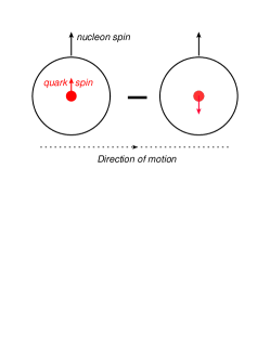
Figure 1: The tensor charge, Eq. (1), measures the net light-front distribution of transversely polarised quarks inside a transversely polarized proton.

The transversity distribution is measurable using Drell-Yan processes in which at least one of the two colliding particles is transversely polarised Barone:2001sp ; but such data is not yet available. Alternatively, the transversity distribution is accessible via semi-inclusive deep-inelastic scattering using transversely polarised targets and also in unpolarised $e^{+}e^{-}$ processes, by studying azimuthal correlations between produced hadrons that appear in opposing jets ($e^{+}e^{-}\to h_{1}h_{2}X$). Capitalising on these observations, the transversity distributions were extracted through an analysis of combined data from the HERMES, COMPASS and Belle collaborations Anselmino:2013vqa ; and those distributions have been used to produce an estimate of the proton’s tensor charges, with the following flavour-separated results:

$$\delta_{T}u=0.39^{+0.18}_{-0.12}\,,\quad\delta_{T}d=-0.25^{+0.30}_{-0.10}\,,$$ (2)

at a renormalisation scale $\zeta_{A}=0.9\,$GeV. Given that the tensor charges are a defining intrinsic property of the nucleon, the magnitude of the errors in Eqs. (2) is unsatisfactory. It is therefore critical to better determine $\delta_{T}u$, $\delta_{T}d$. Consequently, following upgrades at the Thomas Jefferson National Accelerator Facility (JLab), it is anticipated Dudek:2012vr that experiments Gao:2010av ; Avakian:2014aba in Hall-A (SoLID) and Hall-B (CLAS12) will provide a far more precise determination of the tensor charges.

Naturally, measurement of the transversity distribution and the tensor charges will not reveal much about the strong interaction sector of the Standard Model unless these quantities can be calculated using a framework with a traceable connection to QCD. This point is emphasised with particular force by the circumstances surrounding the pion’s valence-quark PDF. As reviewed elsewhere Holt:2010vj , numerous authors suggested that QCD was challenged by a PDF parametrisation based on a precise $\pi N$ Drell-Yan measurement Conway:1989fs . However, the appearance of nonperturbative calculations within the framework of continuum QCD Hecht:2000xa ; Nguyen:2011jy forced reanalyses of the cross-section, with the inclusion of next-to-leading-order evolution Wijesooriya:2005ir and soft-gluon resummation Aicher:2010cb , so that now those claims are known to be false and the pion’s valence-quark PDF may be viewed as a success for QCD Chang:2014lva . The comparisons between experiment and computations of the pion and kaon parton distribution amplitudes and electromagnetic form factors have reached a similar level of understanding Chang:2013nia ; Shi:2014uwa .

Herein, therefore, we compute the proton tensor charges using a confining, symmetry-preserving Dyson-Schwinger equation (DSE) treatment of a single quark-quark interaction; namely, a vector$\,\otimes\,$vector contact-interaction. This approach has proved useful in a variety of contexts, which include meson and baryon spectra, and their electroweak elastic and transition form factors GutierrezGuerrero:2010md ; Roberts:2010rn ; Roberts:2011wy ; Roberts:2011cf ; Wilson:2011aa ; Chen:2012qr ; Chen:2012txa ; Pitschmann:2012by ; Wang:2013wk ; Segovia:2013rca ; Segovia:2013uga . In fact, so long as the momentum of the probe is smaller in magnitude than the dressed-quark mass produced by dynamical chiral symmetry breaking (DCSB), many results obtained in this way are practically indistinguishable from those produced by the most sophisticated interactions that have thus far been employed in DSE studies Roberts:2007jh ; Chang:2011vu ; Bashir:2012fs ; Cloet:2013jya .

It is apposite to remark here that confinement and DCSB are two key features of QCD; and much of the success of the contact-interaction approach owes to its efficacious expression of these emergent phenomena in the Standard Model. They are explained in some detail elsewhere Roberts:2007jh ; Chang:2011vu ; Bashir:2012fs ; Cloet:2013jya so that here we remark only that confinement may be expressed via dynamically-driven changes in the analytic structure of QCD’s propagators and vertices; and DCSB is the origin of more than 98% of the mass of visible material in the Universe. These phenomena are intimately connected; and whereas the nature of confinement is still debated, DCSB is a theoretically established nonperturbative feature of QCD national2012Nuclear , which has widespread, measurable impacts on hadron observables, e.g. Refs. Chen:2012qr ; Pitschmann:2012by ; Chang:2013pq ; Cloet:2013gva ; Roberts:2013mja ; Chang:2013epa ; Gao:2014bca ; Shi:2014uwa ; Segovia:2014aza , so that its expression in QCD is empirically verifiable.

Apart from the hadron physics imperative, the value of the nucleon tensor charges can be directly related to the visible impact of a dressed-quark electric dipole moment (EDM) on neutron and proton EDMs Hecht:2001ry . Novel beyond-the-Standard-Model (BSM) scalar operators may also conceivably be measurable in precision neutron experiments so that one typically considers both the nucleon scalar and tensor charges when exploring bounds on BSM physics Bhattacharya:2011qm . The sum of the scalar charges of all active quark flavours is simply the nucleon $\sigma$-term, which we therefore also compute herein.

Relying on material provided in numerous appendices, we provide a brief outline of our computational framework in Sec. II: both the Faddeev equation treatment of the nucleon and the currents which describe the interaction of a probe with a baryon composed from consistently-dressed constituents. This presentation scheme enables us to embark quickly upon the description and analysis of our results for the scalar and tensor charges, Secs. III and IV, respectively. In Sec. V we use our results for the tensor charges in order to determine the impact of valence-quark EDMs on the neutron and proton EDMs. Section VI is an epilogue.

II Nucleon Faddeev Amplitude and Relevant Interaction Currents

We base our description of the nucleon’s dressed-quark-core on solutions of a Faddeev equation, which is illustrated in Fig. 2, and formulated and described in Apps. A, B. In order to determine the scalar and tensor charges of the nucleon described by this Faddeev equation, the $Q^{2}=0$ values of three interaction currents are needed: elastic electromagnetic, which determines the canonical normalisation of the nucleon’s Faddeev amplitude; scalar; and tensor. The computation of these quantities is detailed in App. C.

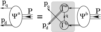
Figure 2: Poincaré covariant Faddeev equation. $\Psi$ is the Faddeev amplitude for a nucleon of total momentum $P=p_{q}+p_{d}$. The shaded rectangle demarcates the kernel of the Faddeev equation: single line, dressed-quark propagator; $\Gamma$, diquark correlation (Bethe-Salpeter) amplitude; and double line, diquark propagator. (See Apps. A, B for details.)

III Sigma-Term

The contribution of a given quark flavour ($q=u,d,\ldots$) to a nucleon’s $\sigma$-term is defined by the matrix element

$$\sigma_{q}=m_{q}\,\langle N(p)|\bar{q}{\mathbb{1}}q|N(p)\rangle\,,$$ (3)

where $|N(p)\rangle$ is the state vector of a nucleon with four-momentum $p$. The $\sigma$-term is independent of the renormalisation scale used in the computation, even though the individual pieces in the product on the right-hand-side (rhs) are not. As explained in App. E, the scale appropriate to our symmetry-preserving regularisation of the contact interaction is $\zeta_{H}\approx M$, where $M$ is the dressed-quark mass.

Our computed value of the nucleon’s $\sigma$-term is reported in Eq. (143); viz.,

$$\sigma_{N}=\sigma_{u}+\sigma_{d}=m\,3.05=21\,{\rm MeV}.$$ (4)

This result is consistent with that obtained using the Feynman-Hellmann theorem in connection with the results from which Ref. Roberts:2011cf was prepared. An interesting way to expose this is to recall Eq. (91), which states that our analysis describes a nucleon that is 77% dressed-quark$\,+\,$scalar-diquark and 23% dressed-quark$\,+\,$axial-vector diquark. In the isospin symmetric limit, which we typically employ, it follows that

$$\sigma_{N} = 0.77\left[\sigma_{Q}+\sigma_{qq^{0}}\right]+0.23\left[\sigma_{Q}+\sigma_{qq^{1}}\right]$$ (5)

$$= \sigma_{Q}+0.77\,\sigma_{qq^{0}}+0.23\,\sigma_{qq^{1}},$$ (6)

where

$$\sigma_{Q} = m\frac{\partial M}{\partial m}=9.6\,{\rm MeV},$$ (7a)

$$\sigma_{qq^{0}} = m\frac{\partial m_{qq^{0}}}{\partial m}=16\,{\rm MeV},$$ (7b)

$$\sigma_{qq^{1}} = m\frac{\partial m_{qq^{1}}}{\partial m}=10\,{\rm MeV},$$ (7c)

again computed using material in Ref. Roberts:2011cf . Inserting Eqs. (7) into Eq. (6), one obtains $\sigma_{N}=24\,$MeV. Apparently, so far as the contribution of explicit chiral symmetry breaking to the mass of the nucleon’s dressed-quark core is concerned, the contact-interaction nucleon is a simple system. This analysis also shows that our diagrammatic computational method is sound; and hence Eq. (4) is the rainbow-ladder (RL) truncation prediction of a vector$\,\otimes\,$vector contact-interaction treated in the Faddeev equation via the static approximation. (Inclusion of meson-baryon loop effects will increase the result in Eq. (4) by approximately 15% Flambaum:2005kc .)

In addition, the fact that Eqs. (4) and (6) yield similar results emphasises the important role of diquark correlations because if the nucleon were just a sum of three massive, weakly-interacting dressed-quarks, then one would have

$$\sigma_{N}^{3M}=3\,\sigma_{Q}=29\,{\rm MeV}\,,$$ (8)

which is 21% too large.

Adopting a different perspective, we note that the value in Eq. (4) is roughly one-half that produced by a Faddeev equation kernel that incorporates scalar and axial-vector diquark correlations in addition to propagators and interaction vertices that possess QCD-like momentum dependence Flambaum:2005kc . It compares similarly with the value inferred in a recent analysis Shanahan:2012wh of lattice-QCD results for octet baryon masses in $2+1$-flavour QCD:

$$\sigma_{N}=45\pm 6\,{\rm MeV}\,.$$ (9)

In order to understand the discrepancy, consider Eqs. (7). The value of $\sigma_{Q}$ matches expectations based on gap equation kernels whose ultraviolet behaviour is consistent with QCD Flambaum:2005kc ; Maris:1999bh . On the other hand, with such interactions one typically finds $\sigma_{qq^{0}}\gtrsim\sigma_{qq^{1}}\gtrsim\sigma_{\rho}=25\,$MeV. We therefore judge that Eq. (4) underestimates the physical value of $\sigma_{N}$; and that the mismatch originates primarily in the rigidity of the diquark Bethe-Salpeter amplitudes produced by the contact interaction, which leads to weaker $m$-dependence of the diquark (and hence nucleon) masses than is obtained with more realistic kernels. Notwithstanding this, Eq. (4) is a useful benchmark, providing a sensible result via a transparent method.

Further valuable information may be obtained from the results in App. C.2 if one supposes that the ratio of contact-interaction $d$- and $u$-quark contributions is more reliable than the net value of $\sigma_{N}$. In this connection, note that for a proton constituted as a weakly interacting system of three massive dressed-quarks in the isospin symmetric limit

$$\frac{\sigma_{N,d}^{3M}}{\sigma_{N,u}^{3M}}=\frac{1}{2}\,.$$ (10)

Comparing this with our computed value

$$\frac{\sigma_{N,d}}{\sigma_{N,u}}=0.65\,,$$ (11)

one learns that diquark correlations work to accentuate the contribution of the singly-represented valence-quark to the proton $\sigma$-term relative to that of doubly-represented valence-quarks: the magnification factor is $1.3$.

Let’s take this another step and assume that $\hat{\sigma}_{N,u}$, $\hat{\sigma}_{N,d}$ in App. C.2 respond weakly to changes in $m$. This is valid so long as solutions of the dressed-quark gap equation satisfy

$$\left.\frac{dM}{dm}\right|_{(m_{u}+m_{d})/2}\stackrel{{\scriptstyle m_{u},m_{d}\ll M}}{{\approx}}\left.\frac{dM}{dm}\right|_{m_{u},m_{d}},$$ (12)

which is found to be a good approximation in all available studies (see, e.g., Refs. Holl:2005st ; Pennington:2010gy ). One may then estimate the effects of isospin symmetry violation owing to the difference between $u$- and $d$-quark current-masses. Taking the value of the mass ratio from Ref. Beringer:1900zz , one finds

$$\frac{m_{u}}{m_{d}}=0.48\pm 0.1\quad\Rightarrow\quad\frac{m_{d}\,\hat{\sigma}_{N,d}}{m_{u}\,\hat{\sigma}_{N,u}}=1.35^{+0.47}_{-0.30}\,.$$ (13)

Alternatively, one might use the mass ratio inferred from a survey of numerical simulations of lattice-regularised QCD Colangelo:2010et , in which case

$$\frac{m_{u}}{m_{d}}=0.47\pm 0.04\quad\Rightarrow\quad\frac{m_{d}\,\hat{\sigma}_{N,d}}{m_{u}\,\hat{\sigma}_{N,u}}=1.38^{+0.17}_{-0.14}\,.$$ (14)

We predict, therefore, that the $d$-quark contribution to that part of the proton’s mass which arises from explicit chiral symmetry breaking is roughly 37% greater than that from the $u$-quark. This value is commensurate with a contemporaneous estimate based on lattice-QCD Erben:2014hza . It is noteworthy that if the proton were a weakly interacting system of three massive dressed-quarks, then Eq. (14) would yield $1.06^{+0.13}_{-0.11}$; and hence one finds again that the presence of diquark correlations within the proton enhances the contribution of $d$-quarks to the proton’s $\sigma$-term.

IV Tensor Charge

The tensor charge associated with a given quark flavour in the proton is defined via the matrix element ($q=u,d,\ldots$)

$$\langle P(p,\sigma)|\bar{q}\sigma_{\mu\nu}q|P(p,\sigma)\rangle=\delta_{T}q\,\bar{\mathpzc u}(p,\sigma)\sigma_{\mu\nu}{\mathpzc u}(p,\sigma)\,,$$ (15)

where ${\mathpzc u}(p,\sigma)$ is a spinor and $|P(p,\sigma)\rangle$ is a state vector describing a proton with momentum $p$ and spin $\sigma$. With $\delta_{T}u$, $\delta_{T}d$ in hand, the isoscalar and isovector tensor charges are readily computed:

$$g_{T}^{(0)}=\delta_{T}u+\delta_{T}d\,,\;g_{T}^{(1)}=\delta_{T}u-\delta_{T}d\,.$$ (16)

Importantly, the tensor charge is a scale-dependent quantity. Its evolution is discussed in App. F.

Our analysis of the proton’s tensor charge in a symmetry-preserving RL-truncation treatment of a vector$\,\otimes\,$vector contact-interaction is detailed in App. C.3. At the model scale, $\zeta_{H}$, which is determined and explained in App. E, we obtain the results in Table C.3, which represent a parameter-free prediction: the current-quark mass and the two parameters that define the interaction were fixed elsewhere Roberts:2011wy , in a study of $\pi$- and $\rho$-meson properties.

It is natural to ask for an estimate of the systematic error in the values reported in Table C.3. As we saw in Sec. III, the error might pessimistically be as much as a factor of two. However, that is an extreme case because, as observed in the Introduction, one generally finds that our treatment of the contact interaction produces results for low-momentum-transfer observables that are practically indistinguishable from those produced by RL studies that employ more sophisticated interactions GutierrezGuerrero:2010md ; Roberts:2010rn ; Roberts:2011cf ; Roberts:2011wy ; Wilson:2011aa ; Chen:2012qr ; Chen:2012txa ; Pitschmann:2012by ; Wang:2013wk ; Segovia:2013rca ; Segovia:2013uga . It is therefore notable that analyses of hadron physics observables using the RL truncation and one-loop QCD renormalisation-group-improved (RGI) kernels for the gap and bound-state equations produce results that are typically within 15% of the experimental value Roberts:2007jh . We therefore ascribe a relative error of 15% to the results in Table C.3 so that our predictions are:

$$\begin{array}[]{l|cccc}&\delta_{T}u&\delta_{T}d&g_{T}^{(0)}&g_{T}^{(1)}\\ \zeta_{H}\approx M&0.69(10)&-0.14(2)&0.55(8)&0.83(12)\end{array}\,.$$ (17)

One means by which to check our error estimate is to repeat the calculations described herein using a modern RGI kernel Qin:2011dd in the gap and bound-state equations. That has not yet been done but one may nevertheless infer what it might yield. Consider first Ref. Yamanaka:2013zoa , which computes the dressed-quark-tensor vertex using a RL-treatment of a QCD-based kernel: one observes that the dressed-quark’s tensor charge is markedly suppressed; namely, with a QCD-based momentum-dependent kernel, a factor of approximately one-half appears on the rhs of Eq. (144). This DCSB-induced suppression would tend to reduce the values in Eq. (17). On the other hand, the use of a more sophisticated momentum-dependent kernel in the bound-state equations increases the amount of dressed-quark orbital angular momentum in the proton, an effect apparent in the reduction of the fraction of proton helicity carried by dressed $u$- and $d$-quarks when one shifts from a contact-interaction framework to a QCD-kindred approach Roberts:2013mja ; Segovia:2014aza . Hence, the tensor charges are determined by two competing effects, the precise balance amongst which can only be revealed by detailed calculations.

In this context, however, it is worth noting that similar DCSB-induced effects are observed in connection with $g_{A}$, the nucleon’s axial charge. The axial-charge of a dressed-quark is suppressed Chang:2012cc , owing to DCSB; but that is compensated in the calculation of $g_{A}$ by dressed-quark orbital angular momentum in the nucleon’s Faddeev wave-function, with the computed value of the nucleon’s axial-charge being 20% larger than that of a dressed-quark. The net effect is that a computation of $g_{A}$ using the framework of Refs. Segovia:2014aza can readily produce a result that is within 15% of the empirical value Roberts:2007jh ; Chang:2012cc . This suggests that our error estimate is reasonable.

The predictions in Eq. (17) are quoted at the model scale, whose value is explained in App. E. In order to make a sensible comparison with estimates obtained in modern simulations of lattice-regularised QCD, those results must be evolved to $\zeta_{2}=2\,$GeV. We therefore list here the results obtained under leading-order evolution to $\zeta_{2}=2\,$GeV, obtained via multiplication by the factor in Eq. (180):

$$\begin{array}[]{l|cccc}&\delta_{T}u&\delta_{T}d&g_{T}^{(0)}&g_{T}^{(1)}\\ \zeta_{2}&0.55(8)&-0.11(2)&0.44(7)&0.66(10)\end{array}\,.$$ (18)

The error in Eq. (180) does not propagate significantly into these results.

Notably, the dominant contribution to $\delta_{T}u$ arises from Diagram 1: tensor probe interacting with a dressed $u$-quark with a scalar diquark as the bystander. The tensor probe interacting with the axial-vector diquark, with a dressed-quark as a spectator, Diagram 4, produces the next largest piece. However, that is largely cancelled by the sum of Diagrams 5 and 6: tensor probe causing a transition between scalar- and axial-vector diquark correlations within the proton whilst the dressed-quark is a bystander. It is a large negative contribution for both $\delta_{T}u$ and $\delta_{T}d$: indeed, owing to a significant cancellation between Diagrams 2 and 4 in the $d$-quark sector, which describe the net result from quark$\,+\,$axial-vector-diquark contributions, the sum of Diagrams 5 and 6 provides almost the entire result for $\delta_{T}d$.

A particularly important result is the impact of the proton’s axial-vector diquark correlation. As determined in App. C.3.6, with a symmetry-preserving treatment of a contact interaction, $\delta_{T}d$ is only nonzero if axial-vector diquark correlations are present. Significantly, in dynamical calculations the strength of axial-vector diquark correlations relative to scalar diquark correlations is a measure of DCSB Chen:2012qr . In the absence of axial-vector diquark correlations [Eqs. (167), Eq. (180)]

$$\begin{array}[]{l|cccc}&\delta_{T\!\not\,1}u&\delta_{T\!\not\,1}d&g_{T\!\not\,1}^{(0)}&g_{T\!\not\,1}^{(1)}\\ \zeta_{2}&0.61(9)&0&0.61(9)&0.61(9)\end{array}\,;$$ (19)

i.e., $\delta_{T}d$ vanishes altogether and $\delta_{T}u$ is increased by 11%. We expect that the influence of axial-vector diquark correlations will be qualitatively similar in the treatment of more sophisticated kernels for the gap and bound-state equations. A hint in support of this expectation may be drawn from the favourable comparison, depicted in Fig. 3, between the predictions for $\delta_{T}u$ in Eq. (19), “4”, and the result of Ref. Hecht:2001ry , “5”. The latter employed a proton and tensor-current that suppressed but did not entirely eliminate the contribution from axial-vector diquark correlations. This same comparison also supports the verity of our error estimate.

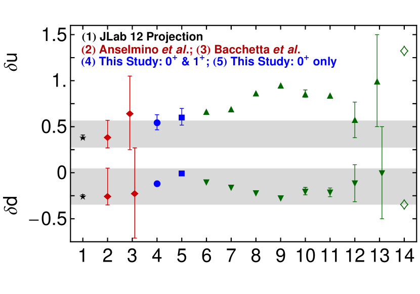
Figure 3: Flavour separation of the proton’s tensor charge: “1” – illustration of anticipated accuracy in planned JLab experiment Gao:2010av , with central values based on Eq. (2); “2” – results in Eq. (2), drawn from Ref. Anselmino:2013vqa ; “3” phenomenological estimate in Ref. Bacchetta:2012ty “4” – prediction herein, Eq. (18); “5” – result obtained herein with omission of axial-vector diquark correlations, Eq. (19); “6-13” – estimates from Refs. Hecht:2001ry ; Cloet:2007em ; Pasquini:2006iv ; Wakamatsu:2007nc ; alexandrou:2014 ; Gockeler:2005cj ; Gamberg:2001qc ; He:1994gz , respectively. By way of context, we note that were the proton a weakly-interacting collection of three massive valence-quarks described by an SU$(4)$-symmetric spin-flavour wave function, then He:1994gz the quark axial and tensor charges are identical, so that $\delta_{T}u=4/3$ and $\delta_{T}d=-1/3$ at the model scale. These values are located at “14”.

Additionally, it is valuable to note that the magnitude of $\delta_{T}u$ is a direct probe of the strength of DCSB and hence of the strong interaction at infrared momenta. This could be anticipated, e.g., from Eqs. (149), (158), the expressions for Diagrams 1 and 4, which produce the dominant positive contributions to $\delta_{T}u$: both show a strong numerator dependence on the dressed-quark mass, $M$; and $M/m\gg 1$ is a definitive signal of DCSB. To quantify the effect, we reduced $\alpha_{\rm IR}$ in the gap and Bethe-Salpeter equations by 20% and recomputed all relevant quantities. This modification reduced the dressed-quark mass by 33%: $M=0.368\to M_{<}=0.246\,$GeV. Combined with knock-on effects throughout all correlations and bound-states, the 20% reduction in $\alpha_{\rm IR}$ produces [Table C.4 and Eq. (180)]

$$\begin{array}[]{l|rrrr}M\to M_{<}&\delta_{T}u&\delta_{T}d&g_{T}^{(0)}&g_{T}^{(1)}\\ \zeta_{2}&0.44&-0.12&0.32&0.56\end{array}\,,$$ (20)

which expresses a 20% decrease in $\delta_{T}u$. As we signalled, the greatest impact of the cut in $\alpha_{\rm IR}$ and hence $M$ is a reduction in the size of the contributions from Diagrams 1 and 4: the former describes the tensor probe interacting with a dressed-quark whilst a scalar diquark is a spectator; and the latter involves a tensor probe exploring an axial-vector diquark with a dressed-quark bystander.

As remarked in the Introduction, the tensor charge is a defining intrinsic property of the proton and hence there is great interest in its reliable experimental and theoretical determination. In Fig. 3 we therefore compare our predictions with results from other analyses Hecht:2001ry ; Bacchetta:2012ty ; Cloet:2007em ; Pasquini:2006iv ; Wakamatsu:2007nc ; alexandrou:2014 ; Gockeler:2005cj ; Gamberg:2001qc ; He:1994gz . Evidently, of all available computations, our contact-interaction predictions are in best agreement with the phenomenological estimates in Eq. (2).

Another interesting point is highlighted by a comparison between our predictions and the values obtained when the proton is considered to be a weakly-interacting collection of three massive valence-quarks described by an SU$(4)$-symmetric spin-flavour wave function He:1994gz : $\delta_{T}^{{\rm SU}(4)}u=2e_{u}$ and $\delta_{T}^{{\rm SU}(4)}d=e_{d}$ cf. our results, Eq. (17), $\delta_{T}u=0.52(2e_{u})$, $\delta_{T}d=0.42(e_{d})$. The presence of diquark correlations in the proton amplitude significantly suppresses the magnitude of the tensor charge associated with each valence quark whilst simultaneously increasing the ratio $\delta_{T}d/\delta_{T}u$ by approximately 20%.

V Electric Dipole Moments

In typical extensions of the Standard Model, quarks acquire an EDM Pospelov:2005pr ; RamseyMusolf:2006vr ; i.e., an interaction with the photon that proceeds via a current of the form:

$$\tilde{d}_{q}\,q\gamma_{5}\sigma_{\mu\nu}q\,,$$ (21)

where $\tilde{d}_{q}$ is the quark’s EDM and here we consider $q=u,d$. The EDM of a proton containing quarks which interact in this way is defined as follows:

$$\langle P(p,\sigma)|\mathcal{J}_{\mu\nu}^{\text{EDM}}|P(p,\sigma)\rangle=\tilde{d}_{p}\,\bar{\mathpzc u}(p,\sigma)\gamma_{5}\sigma_{\mu\nu}{\mathpzc u}(p,\sigma)\,,$$ (22)

where

$$\mathcal{J}_{\mu\nu}^{\text{EDM}}(x)=\tilde{d}_{u}\,\bar{u}(x)\gamma_{5}\sigma_{\mu\nu}u(x)+\tilde{d}_{d}\,\bar{d}(x)\gamma_{5}\sigma_{\mu\nu}d(x)\,.$$ (23)

At this point it is useful to recall a simple Dirac-matrix identity:

$$\gamma_{5}\sigma_{\mu\nu}=\frac{1}{2}\varepsilon_{\mu\nu\alpha\beta}\sigma_{\alpha\beta}\,,$$ (24)

using which one can write

$$\mathcal{J}_{\mu\nu}^{\text{EDM}}=\frac{1}{2}\varepsilon_{\mu\nu\alpha\beta}\left[\tilde{d}_{u}\,\bar{u}\sigma_{\alpha\beta}u+\tilde{d}_{d}\,\bar{d}\sigma_{\alpha\beta}d\right]\,.$$ (25)

It follows that

$$\langle P(p,\sigma)|\mathcal{J}_{\mu\nu}^{\text{EDM}}|P(p,\sigma)\rangle$$

$$=\frac{1}{2}\varepsilon_{\mu\nu\alpha\beta}\left[\tilde{d}_{u}\,\delta_{T}u\,+\tilde{d}_{d}\,\delta_{T}d\,\right]\bar{\mathpzc u}(p,\sigma)\sigma_{\alpha\beta}{\mathpzc u}(p,\sigma)$$ (26)

$$=\left[\tilde{d}_{u}\,\delta_{T}u\,+\tilde{d}_{d}\,\delta_{T}d\,\right]\bar{\mathpzc u}(p,\sigma)\gamma_{5}\sigma_{\mu\nu}{\mathpzc u}(p,\sigma)\,;$$ (27)

namely, the quark-EDM contribution to a proton’s EDM is completely determined once the proton’s tensor charges are known:

$$\tilde{d}_{p}=\tilde{d}_{u}\,\delta_{T}u\,+\tilde{d}_{d}\,\delta_{T}d\,.$$ (28)

With emerging techniques, it is becoming possible to place competitive upper-limits on the proton’s EDM using storage rings in which polarized particles are exposed to an electric field Pretz:2013us .

An analogous result for the neutron is readily inferred. In the limit of isospin symmetry,

$$\langle N(p,\sigma)|\bar{u}\sigma_{\mu\nu}u|N(p,\sigma)\rangle =\langle P(p,\sigma)|\bar{d}\sigma_{\mu\nu}d|P(p,\sigma)\rangle\,,$$

$$\langle N(p,\sigma)|\bar{d}\sigma_{\mu\nu}d|N(p,\sigma)\rangle =\langle P(p,\sigma)|\bar{u}\sigma_{\mu\nu}u|P(p,\sigma)\rangle\,;$$ (29)

and hence

$$\tilde{d}_{n}=\tilde{d}_{u}\,\delta_{T}d\,+\tilde{d}_{d}\,\delta_{T}u\,.$$ (30)

Using the results in Eq. (17), we therefore have

$$\tilde{d}_{n}=-0.14\,\tilde{d}_{u}+0.69\,\tilde{d}_{d}\,,\;\tilde{d}_{p}=0.69\,\tilde{d}_{u}-0.14\,\tilde{d}_{d}\,.$$ (31)

It is worth contrasting Eqs. (31) with the results one would obtain by assuming that the nucleon is merely a collection of three massive valence-quarks described by an SU$(4)$-symmetric spin-flavour wave function. Then, by analogy with magnetic moment computations, a procedure also made valid by Eq. (24):

$$\tilde{d}_{n}=-\frac{1}{3}\,\tilde{d}_{u}+\frac{4}{3}\,\tilde{d}_{d}\,,\;\tilde{d}_{p}=\frac{4}{3}\,\tilde{d}_{u}-\frac{1}{3}\,\tilde{d}_{d}\,,$$ (32)

values which are roughly twice the size that we obtain.

The impact of our predictions for the scalar and tensor charges on BSM phenomenology may be elucidated, e.g., by following the analysis in Refs. Bhattacharya:2011qm ; Dekens:2014jka .

VI Conclusion

We employed a confining, symmetry-preserving, Dyson-Schwinger equation treatment of a vector$\,\otimes\,$vector contact interaction in order to compute the dressed-quark-core contribution to the nucleon $\sigma$-term and tensor charges. The latter enabled us to determine the effect of dressed-quark electric dipole moments (EDMs) on the neutron and proton EDMs.

A characteristic feature of DSE treatments of ground-state baryons is the predicted presence of strong scalar and axial-vector diquark correlations within these bound-states. Indeed, in some respects the baryons can be viewed as weakly interacting dressed-quark$\,+\,$diquark composites. The diquark correlations are active participants in all scattering events and therefore serve to modify the contribution to observables of the singly-represented valence-quark relative to that of the doubly-represented quark.

Regarding our analysis of the proton’s $\sigma$-term, we estimate that with a realistic $d$-$u$ mass splitting, the singly-represented $d$-quark contributes 37% more than the doubly-represented $u$-quark to that part of the proton mass which owes to explicit chiral symmetry breaking [Eqs. (13), (14)].

Our predictions for the proton’s tensor charges, $\delta_{T}u$, $\delta_{T}d$, are presented in Eq. (18). In this case, compared to results obtained in simple quark models, diquark correlations act to reduce the size of $\delta_{T}u$, $\delta_{T}d$ by a factor of two and increase the ratio $\delta_{T}d/\delta_{T}u$ by roughly 20%. Two additional observations are particularly significant. First, the magnitude of $\delta_{T}u$ is a direct measure of the strength of DCSB in the Standard Model, diminishing rapidly with the difference between the scales of dynamical and explicit chiral symmetry breaking. Second, $\delta_{T}d$ measures the strength of axial-vector diquark correlations in the proton, vanishing with $P_{1^{+}}/P_{0^{+}}$; i.e., the ratio of axial-vector- and scalar-diquark interaction probabilities, which is also a measure of DCSB.

Our analysis of the Faddeev equation employed a simplifying truncation; viz., a variant of the so-called static approximation. A natural next step is recalculation of the tensor charges after eliminating that truncation. Subsequently or simultaneously, one might also employ the approaches of Refs. Eichmann:2013afa ; Segovia:2014aza in order to obtain DSE predictions with a more direct connection to QCD.

Appendix A Contact interaction

Our treatment of the contact interaction begins with the gap equation

$$S(p)^{-1}=i\gamma\cdot p+m$$ (33)

$$+\!\!\int\!\frac{d^{4}q}{(2\pi)^{4}}g^{2}D_{\mu\nu}(p-q)\frac{\lambda^{a}}{2}\gamma_{\mu}S(q)\frac{\lambda^{a}}{2}\Gamma_{\nu}(q,p),\;$$

wherein $m$ is the Lagrangian current-quark mass, $D_{\mu\nu}$ is the vector-boson propagator and $\Gamma_{\nu}$ is the quark–vector-boson vertex. We work with the choice

$$g^{2}D_{\mu\nu}(p-q)=\delta_{\mu\nu}\frac{4\pi\alpha_{\rm IR}}{m_{G}^{2}}\,,$$ (34)

where $m_{G}=0.8\,$GeV is a gluon mass-scale typical of the one-loop renormalisation-group-improved interaction introduced in Ref. Qin:2011dd , and the fitted parameter $\alpha_{\rm IR}/\pi=0.93$ is commensurate with contemporary estimates of the zero-momentum value of a running-coupling in QCD Aguilar:2010gm ; Boucaud:2010gr . Equation (34) is embedded in a rainbow-ladder (RL) truncation of the DSEs, which is the leading-order in the most widely used, global-symmetry-preserving truncation scheme Munczek:1994zz ; Bender:1996bb . This means

$$\Gamma_{\nu}(p,q)=\gamma_{\nu}$$ (35)

in Eq. (33) and in the subsequent construction of the Bethe-Salpeter kernels.

One may view the interaction in Eq. (34) as being inspired by models of the Nambu–Jona-Lasinio type Nambu:1961tp . However, our treatment is atypical. Moreover, as noted in the Introduction, one normally finds Eqs. (34), (35) produce results for low-momentum-transfer observables that are practically indistinguishable from those produced by more sophisticated interactions GutierrezGuerrero:2010md ; Roberts:2010rn ; Roberts:2011cf ; Roberts:2011wy ; Wilson:2011aa ; Chen:2012qr ; Chen:2012txa ; Pitschmann:2012by ; Wang:2013wk ; Segovia:2013rca ; Segovia:2013uga . Using Eqs. (34), (35), the gap equation becomes

$$S^{-1}(p)=i\gamma\cdot p+m+\frac{16\pi}{3}\frac{\alpha_{\rm IR}}{m_{G}^{2}}\int\!\frac{d^{4}q}{(2\pi)^{4}}\,\gamma_{\mu}\,S(q)\,\gamma_{\mu}\,,$$ (36)

an equation in which the integral possesses a quadratic divergence. When the divergence is regularised in a Poincaré covariant manner, the solution is

$$S(p)^{-1}=i\gamma\cdot p+M\,,$$ (37)

where $M$ is momentum-independent and determined by

$$M=m+M\frac{4\alpha_{\rm IR}}{3\pi m_{G}^{2}}\int_{0}^{\infty}\!ds\,s\,\frac{1}{s+M^{2}}\,.$$ (38)

We define Eq. (36) by writing Ebert:1996vx

$$\frac{1}{s+M^{2}} = \int_{0}^{\infty}d\tau\,{\rm e}^{-\tau(s+M^{2})}$$ (40)

$$\rightarrow \int_{\tau_{\rm uv}^{2}}^{\tau_{\rm ir}^{2}}d\tau\,{\rm e}^{-\tau(s+M^{2})}$$

$$=\frac{{\rm e}^{-(s+M^{2})\tau_{\rm uv}^{2}}-e^{-(s+M^{2})\tau_{\rm ir}^{2}}}{s+M^{2}}\,,$$

where $\tau_{\rm ir,uv}$ are, respectively, infrared and ultraviolet regulators. It is apparent from Eq. (40) that a finite value of $\tau_{\rm ir}=:1/\Lambda_{\rm ir}$ implements confinement by ensuring the absence of quark production thresholds Krein:1990sf . Since Eq. (34) does not define a renormalisable theory, then $\Lambda_{\rm uv}:=1/\tau_{\rm uv}$ cannot be removed but instead plays a dynamical role, setting the scale of all dimensioned quantities. Using Eq. (40), the gap equation becomes

$$M=m+M\frac{4\alpha_{\rm IR}}{3\pi m_{G}^{2}}\,\,{\cal C}^{\rm iu}(M^{2})\,,$$ (41)

where,

$$\mathcal{C}^{\text{iu}}(\omega) =\omega\,[\Gamma(-1,\omega\tau_{\rm uv}^{2})-\Gamma(-1,\omega\tau_{\rm ir}^{2})]\,,$$ (42)

with $\Gamma(\alpha,y)$ being the incomplete gamma-function.

At this point we also list expressions for the other regularised integrals that we employ herein:

$$\mathcal{C}_{n}^{\text{iu}}(\omega) =(-1)^{n}\frac{\omega^{n}}{n!}\frac{d^{n}}{d\omega^{n}}\,\mathcal{C}^{\text{iu}}(\omega)\,,$$ (43)

$$\mathcal{D}^{\rm iu}(\omega) =\int_{R}ds\,\frac{s^{2}}{s+M^{2}}$$

$$=2\omega^{2}\,[\Gamma(-2,\omega\tau_{\rm uv}^{2})-\Gamma(-2,\omega\tau_{\rm ir}^{2})]\,,$$ (44)

$$\mathcal{E}^{\rm iu}(\omega) =\int_{R}ds\,\frac{s^{3}}{s+M^{2}}$$

$$=6\omega^{3}\,[\Gamma(-3,\omega\tau_{\rm uv}^{2})-\Gamma(-3,\omega\tau_{\rm ir}^{2})]\,,$$ (45)

$$\check{\mathcal{G}}_{1}^{\rm iu}(\omega) =\int_{R}ds\,\frac{s}{\left(s+\omega\right)^{3}}=\frac{1}{2}\frac{d^{2}}{d\omega^{2}}\,\mathcal{C}^{\text{iu}}(\omega)\,,$$ (46)

$$\check{\mathcal{G}}_{2}^{\rm iu}(\omega) =\int_{R}ds\,\frac{s^{2}}{\left(s+\omega\right)^{3}}$$

$$=\bar{\mathcal{C}}_{1}^{\text{iu}}(\omega)-\frac{\omega}{2}\frac{d^{2}}{d\omega^{2}}\,\mathcal{C}^{\text{iu}}(\omega)\,,$$ (47)

$$\check{\mathcal{G}}_{3}^{\rm iu}(\omega) =\int_{R}ds\,\frac{s^{3}}{\left(s+\omega\right)^{3}}$$

$$=\mathcal{C}^{\text{iu}}(\omega)-2\,\mathcal{C}_{1}^{\text{iu}}(\omega)+\mathcal{C}_{2}^{\text{iu}}(\omega)\,,$$ (48)

$$\check{\mathcal{G}}_{4}^{\rm iu}(\omega) =\int_{R}ds\,\frac{s^{4}}{\left(s+\omega\right)^{3}}=\mathcal{D}^{\rm iu}(\omega)$$

$$\quad-2\omega\,\mathcal{C}^{\text{iu}}(\omega)+3\omega\,\mathcal{C}_{1}^{\text{iu}}(\omega)-\omega\,\mathcal{C}_{2}^{\text{iu}}(\omega)\,,$$ (49)

$$\check{\mathcal{G}}_{5}^{\rm iu}(\omega) =\int_{R}ds\,\frac{s^{5}}{\left(s+\omega\right)^{3}}=\mathcal{E}^{\rm iu}(\omega)-2\omega\,\mathcal{D}^{\rm iu}(\omega)$$

$$\quad+3\omega^{2}\,\mathcal{C}^{\text{iu}}(\omega)-4\omega^{2}\,\mathcal{C}_{1}^{\text{iu}}(\omega)+\omega^{2}\,\mathcal{C}_{2}^{\text{iu}}(\omega)\,,$$ (50)

where $\{{\mathcal{G}}_{i}=\check{\mathcal{G}}_{i}/(16\pi^{2})$, $i=1,\ldots,5\}$.

The parameters that specify our treatment of the contact interaction were determined in a study of $\pi$- and $\rho$-meson properties Roberts:2011wy ; viz., $\alpha_{\rm IR}/\pi=0.93$ and (in GeV)

$$m=0.007\,,\;\Lambda_{\rm ir}=0.240\,\;\Lambda_{\rm uv}=0.905\,,$$ (51)

using which, Eq. (41) yields

$$M=0.368\,{\rm GeV}.$$ (52)

With the aim of exploring the impact of DCSB on our results, herein we also consider results obtained with $\alpha_{\rm IR}/\pi=0.74$, in which case

$$M\to M_{<}=0.246\,{\rm GeV}.$$ (53)

Appendix B Faddeev Equation

We describe the dressed-quark-cores of the nucleon via solutions of a Poincaré-covariant Faddeev equation Cahill:1988dx . The equation is derived following upon the observation that an interaction which describes mesons also generates quark-quark (diquark) correlations in the colour-$\bar{3}$ channel Cahill:1987qr . The fidelity of the diquark approximation to the quark-quark scattering kernel has been verified Eichmann:2011vu .

In RL truncation, the colour-antitriplet diquark correlations are described by an homogeneous Bethe-Salpeter equation that is readily inferred from the analogous meson equation; viz., following Ref. Cahill:1987qr and expressing the diquark amplitude as

$$\Gamma^{c}_{qq}(k;P)=\Gamma_{qq}(k;P)C^{\dagger}H^{c},$$ (54)

with

$$\{H^{1}=i\lambda^{7},H^{2}=-i\lambda^{5},H^{3}=i\lambda^{2}\}\,,\epsilon_{c_{1}c_{2}c_{3}}=(H^{c_{3}})_{c_{1}c_{2}}\,,$$ (55)

where $\{\lambda^{2,5,7}\}$ are Gell-Mann matrices, then

$$\Gamma_{qq}(k;P)=-\frac{8\pi}{3}\frac{\alpha_{\rm IR}}{m_{G}^{2}}\int\!\frac{d^{4}q}{(2\pi)^{4}}\,\gamma_{\mu}\chi_{qq}(q;P)\gamma_{\mu}\,,$$ (56)

where $\chi_{qq}(q;P)=S(q)\Gamma_{qq}(P)S(q-P)$ and $\Gamma_{qq}$ is the diquark Bethe-Salpeter amplitude, which is independent of the relative momentum when using a contact interaction Roberts:2011wy .

Scalar and axial-vector quark-quark correlations are dominant in studies of the nucleon:

$$\Gamma^{0^{+}}_{qq}(P) = i\gamma_{5}E_{qq0}(P)+\frac{1}{M}\gamma_{5}\gamma\cdot PF_{qq0}(P)\,,\rule{20.00003pt}{0.0pt}$$ (57)

$$i\Gamma_{qq\,\mu}^{1^{+}}(P) = i\gamma^{T}_{\mu}E_{qq1}(P),$$ (58)

where $P_{\mu}\gamma^{T}_{\mu}=0$. These amplitudes are canonically normalised:

$$P_{\mu}=2{\rm tr}\!\!\int\frac{d^{4}q}{(2\pi)^{4}}\Gamma_{qq}^{0^{+}}(-P)\frac{\partial}{\partial P_{\mu}}S(q+P)\Gamma_{qq}^{0^{+}}(P)S(q);$$ (59)

and

$$P_{\mu}=\frac{2}{3}{\rm tr}\!\!\int\frac{d^{4}q}{(2\pi)^{4}}\Gamma_{qq\,\alpha}^{1^{+}}(-P)\frac{\partial}{\partial P_{\mu}}S(q+P)\Gamma_{qq\,\alpha}^{1^{+}}(P)S(q).$$ (60)

A $J=\frac{1}{2}$ baryon is represented by a Faddeev amplitude

$$\Psi=\Psi_{1}+\Psi_{2}+\Psi_{3}\,,$$ (61)

where the subscript identifies the bystander quark and, e.g., $\Psi_{1,2}$ are obtained from $\Psi_{3}$ by a cyclic permutation of all the quark labels. We employ a simple but realistic representation of $\Psi$. The spin- and isospin-$\frac{1}{2}$ nucleon is a sum of scalar and axial-vector diquark correlations:

$$\Psi_{3}(p_{i},\alpha_{i},\tau_{i})={\cal N}_{3}^{0^{+}}+{\cal N}_{3}^{1^{+}},$$ (62)

with $(p_{i},\alpha_{i},\tau_{i})$ the momentum, spin and isospin labels of the quarks constituting the bound state, and $P=p_{1}+p_{2}+p_{3}$ the system’s total momentum.

The scalar diquark piece in Eq. (62) is

$${\cal N}_{3}^{0^{+}}(p_{i},\alpha_{i},\tau_{i}) =[\Gamma^{0^{+}}(\frac{1}{2}p_{[12]};K)]_{\alpha_{1}\alpha_{2}}^{\tau_{1}\tau_{2}}$$

$$\quad\times\Delta^{0^{+}}(K)\,[{\cal S}(\ell;P){\mathpzc u}(P)]_{\alpha_{3}}^{\tau_{3}},$$ (63)

where: the spinor satisfies Eq. (184), with $M$ the mass obtained by solving the Faddeev equation, and it is also a spinor in isospin space with $\varphi_{+}={\rm col}(1,0)$ for the charge-one state and $\varphi_{-}={\rm col}(0,1)$ for the neutral state; $K=p_{1}+p_{2}=:p_{\{12\}}$, $p_{[12]}=p_{1}-p_{2}$, $\ell:=(-p_{\{12\}}+2p_{3})/3$;

$$\Delta^{0^{+}}(K)=\frac{1}{K^{2}+m_{qq_{0^{+}}}^{2}}$$ (64)

is a propagator for the scalar diquark formed from quarks $1$ and $2$, with $m_{qq_{0^{+}}}$ the mass-scale associated with this correlation, and $\Gamma^{0^{+}}\!$ is the canonically-normalised Bethe-Salpeter amplitude described above; and ${\cal S}$, a $4\times 4$ Dirac matrix, describes the relative quark-diquark momentum correlation.

The axial-vector component in Eq. (62) is

$${\cal N}^{1^{+}}(p_{i},\alpha_{i},\tau_{i}) =[{\tt t}^{i}\,\Gamma_{\mu}^{1^{+}}(\frac{1}{2}p_{[12]};K)]_{\alpha_{1}\alpha_{2}}^{\tau_{1}\tau_{2}}$$

$$\quad\times\Delta_{\mu\nu}^{1^{+}}(K)\,[{\cal A}^{i}_{\nu}(\ell;P){\mathpzc u}(P)]_{\alpha_{3}}^{\tau_{3}}\,,$$ (65)

where the symmetric isospin-triplet matrices are

$${\tt t}^{+}=\frac{1}{\surd 2}(\tau^{0}+\tau^{3})\,,\;{\tt t}^{0}=\tau^{1}\,,\;{\tt t}^{-}=\frac{1}{\surd 2}(\tau^{0}-\tau^{3})\,,$$ (66)

and the other elements in Eq. (65) are straightforward generalisations of those in Eq. (63) with, e.g.,

$$\Delta_{\mu\nu}^{1^{+}}(K)=\frac{1}{K^{2}+m_{qq_{1^{+}}}^{2}}\,\left(\delta_{\mu\nu}+\frac{K_{\mu}K_{\nu}}{m_{qq_{1^{+}}}^{2}}\right)\,.$$ (67)

One can now write the Faddeev equation for $\Psi_{3}$:

$$\left[\begin{array}[]{r}{\cal S}(k;P)\,{\mathpzc u}(P)\\ {\cal A}^{i}_{\mu}(k;P)\,{\mathpzc u}(P)\end{array}\right]$$ (70)

$$= -\,4\,\int\frac{d^{4}\ell}{(2\pi)^{4}}\,{\cal M}(k,\ell;P)\left[\begin{array}[]{r}{\cal S}(\ell;P)\,{\mathpzc u}(P)\\ {\cal A}^{j}_{\nu}(\ell;P)\,{\mathpzc u}(P)\end{array}\right].\rule{10.00002pt}{0.0pt}$$ (73)

The kernel in Eq. (73) is

$${\cal M}(k,\ell;P)=\left[\begin{array}[]{cc}{\cal M}_{00}&({\cal M}_{01})^{j}_{\nu}\\ ({\cal M}_{10})^{i}_{\mu}&({\cal M}_{11})^{ij}_{\mu\nu}\rule{0.0pt}{12.91663pt}\end{array}\right],$$ (74)

with

$${\cal M}_{00} = \Gamma^{0^{+}}\!(k_{q}-\ell_{qq}/2;\ell_{qq})\,S^{\rm T}(\ell_{qq}-k_{q})$$ (75)

$$\times\,\bar{\Gamma}^{0^{+}}\!(\ell_{q}-k_{qq}/2;-k_{qq})\,S(\ell_{q})\,\Delta^{0^{+}}(\ell_{qq})\,,\rule{20.00003pt}{0.0pt}$$

where: $\ell_{q}=\ell$, $k_{q}=k$, $\ell_{qq}=-\ell+P$, $k_{qq}=-k+P$, the superscript “T” denotes matrix transpose, $\bar{\Gamma}$ is defined in Eq. (189); and

$$({\cal M}_{01})^{j}_{\nu} = {\tt t}^{j}\,\Gamma_{\mu}^{1^{+}}\!(k_{q}-\ell_{qq}/2;\ell_{qq})S^{\rm T}(\ell_{qq}-k_{q})\,$$ (76)

$$\rule{-15.00002pt}{0.0pt}\times\bar{\Gamma}^{0^{+}}\!(\ell_{q}-k_{qq}/2;-k_{qq})\,S(\ell_{q})\,\Delta^{1^{+}}_{\mu\nu}(\ell_{qq}),\rule{22.0pt}{0.0pt}$$

$$({\cal M}_{10})^{i}_{\mu} = \Gamma^{0^{+}}\!(k_{q}-\ell_{qq}/2;\ell_{qq})\,S^{\rm T}(\ell_{qq}-k_{q})\,{\tt t}^{i}\,$$ (77)

$$\rule{-15.00002pt}{0.0pt}\times\bar{\Gamma}_{\mu}^{1^{+}}\!(\ell_{q}-k_{qq}/2;-k_{qq})\,S(\ell_{q})\,\Delta^{0^{+}}(\ell_{qq}),\rule{22.0pt}{0.0pt}$$

$$({\cal M}_{11})^{ij}_{\mu\nu} = {\tt t}^{j}\,\Gamma_{\rho}^{1^{+}}\!(k_{q}-\ell_{qq}/2;\ell_{qq})\,S^{\rm T}(\ell_{qq}-k_{q})\,{\tt t}^{i}\,$$ (78)

$$\rule{-15.00002pt}{0.0pt}\times\bar{\Gamma}^{1^{+}}_{\mu}\!(\ell_{q}-k_{qq}/2;-k_{qq})\,S(\ell_{q})\,\Delta^{1^{+}}_{\rho\nu}(\ell_{qq}).\rule{22.0pt}{0.0pt}$$

The dressed-quark propagator is described in Sec. A and the diquark propagators are given in Eqs. (64), (67), so the Faddeev equation is complete once the diquark Bethe-Salpeter amplitudes are computed from Eqs. (56) – (60). However, we follow Ref. Roberts:2011cf and employ a simplification of the kernel; viz., in the Faddeev equation, the quark exchanged between the diquarks is represented as

$$S^{\rm T}(k)\to\frac{g_{N}^{2}}{M}\,,$$ (79)

where $g_{N}=1.18$. This is a variant of the so-called “static approximation,” which itself was introduced in Ref. Buck:1992wz and has subsequently been used in studying a range of nucleon properties Bentz:2007zs . In combination with diquark correlations generated by Eq. (34), whose Bethe-Salpeter amplitudes are momentum-independent, Eq. (79) generates Faddeev equation kernels which themselves are momentum-independent. The dramatic simplifications which this produces are the merit of Eq. (79). Nevertheless, we are currently exploring the veracity of this truncation.

The general forms of the matrices ${\cal S}(\ell;P)$ and ${\cal A}^{i}_{\nu}(\ell;P)$, which describe the momentum-space correlation between the quark and diquark in the nucleon, are described in Refs. Oettel:1998bk ; Cloet:2007pi . However, with the interaction described in Sec. A augmented by Eq. (79), they simplify greatly; viz.,

$${\cal S}(P) = s(P)\,{\mathbb{1}}\,,$$ (80a)

$$i{\cal A}^{j}_{\mu}(P) = a_{1}^{j}(P)\gamma_{\mu}\gamma_{5}+ia_{2}^{j}(P)\gamma_{5}\hat{P}_{\mu}\,,j=+,0\,,\rule{20.00003pt}{0.0pt}$$ (80b)

with the scalars $s$, $a_{1,2}^{i}$ independent of the relative quark-diquark momentum and $\hat{P}^{2}=-1$.

The mass of the ground-state nucleon is then determined by a $5\times 5$ matrix Faddeev equation; viz., $\Psi=K\Psi$, with the eigenvector defined via

$$\Psi(P)^{\rm T}=\left[s(P)\;a_{1}^{+}(P)\;a_{1}^{0}(P)\;a_{2}^{+}(P)\;a_{2}^{0}(P)\right],$$ (81)

and the kernel $({\mathpzc k}_{\pm}=\pm\surd 2)$

$$K(P)=$$

$$\left[\begin{array}[]{ccccc}K^{00}_{ss}&{\mathpzc k}_{-}\,K^{01}_{sa_{1}}&K^{01}_{sa_{1}}&{\mathpzc k}_{-}\,K^{01}_{sa_{2}}&K^{01}_{sa_{2}}\\[3.01385pt] {\mathpzc k}_{-}\,K^{10}_{a_{1}s}&0&{\mathpzc k}_{+}\,K^{11}_{a_{1}a_{1}}&0&{\mathpzc k}_{+}\,K^{11}_{a_{1}a_{2}}\\[3.01385pt] K^{10}_{a_{1}s}&{\mathpzc k}_{+}\,K^{11}_{a_{1}a_{1}}&K^{11}_{a_{1}a_{1}}&{\mathpzc k}_{+}\,K^{11}_{a_{1}a_{2}}&K^{11}_{a_{1}a_{2}}\\[3.01385pt] {\mathpzc k}_{-}\,K^{10}_{a_{2}s}&0&{\mathpzc k}_{+}\,K^{11}_{a_{2}a_{1}}&0&{\mathpzc k}_{+}\,K^{11}_{a_{2}a_{2}}\\[3.01385pt] K^{10}_{a_{2}s}&{\mathpzc k}_{+}\,K^{11}_{a_{2}a_{1}}&K^{11}_{a_{2}a_{1}}&{\mathpzc k}_{+}\,K^{11}_{a_{2}a_{2}}&K^{11}_{a_{2}a_{2}}\end{array}\right],$$ (87)

whose entries are given explicitly in Eqs. (B20), (B21) of Ref. Wilson:2011aa . Given the structure of the kernel, the eigenvectors exhibit the pattern:

$$a_{i}^{+}=-\sqrt{2}a_{i}^{0},\;i=1,2.$$ (88)

Using the parameters and results described in and connection with Eqs. (51), (52), the diquark Bethe-Salpeter equations produce the following diquark masses (in GeV)

$$m_{qq{0^{+}}}=0.78\,,\;m_{qq{1^{+}}}=1.06\,,$$ (89)

and canonically normalised amplitudes:

$$E_{qq{0^{+}}}=2.742\,,\;F_{qq{0^{+}}}=0.314\,,\;E_{qq{1^{+}}}=1.302\,.$$ (90)

With this input to the Faddeev equation, one obtains Roberts:2011cf ; Wilson:2011aa ; Chen:2012qr $m_{N}=1.14\,$GeV and the following unit-normalised eigenvector

$$\begin{array}[]{ccccc}s(P)&a_{1}^{+}(P)&a_{1}^{0}(P)&a_{2}^{+}(P)&a_{2}^{0}(P)\\ 0.88&-0.38&0.27&-0.065&0.046\end{array}\,.$$ (91)

As explained elsewhere Roberts:2011cf ; Wilson:2011aa ; Chen:2012qr , the mass is greater than that determined empirically because our Faddeev equation kernel omits resonant contributions; i.e., does not contain effects that may phenomenologically be associated with a meson cloud. It is for this reason that our Faddeev equation describes the nucleon’s dressed-quark core. Notably, meson cloud effects typically work to reduce a hadron’s mass Hecht:2002ej .

Using the reduced coupling value described in connection with Eq. (53), the diquark Bethe-Salpeter equations produce the following diquark masses (in GeV)

$$m_{qq{0^{+}}}=0.70\,,\;m_{qq{1^{+}}}=0.98\,,$$ (92)

and canonically normalised amplitudes:

$$E_{qq{0^{+}}}=2.165\,,\;F_{qq{0^{+}}}=0.139\,,\;E_{qq{1^{+}}}=1.093\,.$$ (93)

With this input to the Faddeev equation, one obtains $m_{N}=1.02\,$GeV and the following unit-normalised eigenvector

$$\begin{array}[]{ccccc}s(P)&a_{1}^{+}(P)&a_{1}^{0}(P)&a_{2}^{+}(P)&a_{2}^{0}(P)\\ 0.88&-0.38&0.27&-0.065&0.046\end{array}\,.$$ (94)

Plainly, a 20% cut in the infrared value of the coupling diminishes the strength of DCSB by 33%. This feeds into reductions of the diquark Bethe-Salpeter amplitudes and a 10% cut in the nucleon mass. On the other hand, the nucleon’s Faddeev amplitude, which describes its internal structure, is almost unchanged. The same pattern is seen in studies of the temperature dependence of nucleon properties Wang:2013wk .

Appendix C Interaction Currents

In order to translate the diagrams drawn in this Appendix into formulae, it is helpful to bear the following points in mind.

(1) In front of a closed fermion trace; i.e., a vertex, one should, as usual, include a factor of $(-1)$.

(2a) States entering a diagram are described by the amplitudes

$$\Gamma_{qq}^{0^{+}}(P) =\gamma_{5}\,(iE_{qq0^{+}}+\frac{1}{M}\,\gamma\cdot P\,F_{qq0^{+}})\,,$$ (95a)

$$\Gamma_{qq\mu}^{1^{+}}(P) =iE_{qq1^{+}}\gamma_{\mu}^{T}\,,$$ (95b)

$$\mathcal{S}(P)\, =s\,{\mathbb{1}}\,,$$ (95c)

$$\mathcal{A}_{\mu}^{j}(P) =a_{1}^{j}\gamma_{\mu}\gamma_{5}+ia_{2}^{j}\gamma_{5}\hat{P}_{\mu}\,.$$ (95d)

(N.B. In this Appendix we have absorbed the “$i$” of Eqs. (58), (80) into the labels $\Gamma_{qq\mu}^{1^{+}}(P)$ and $\mathcal{A}_{\mu}^{j}$.)

(2b) States leaving a diagram are described by the amplitudes

$$\Gamma_{qq}^{0^{+}}(-P) =\gamma_{5}\,(iE_{qq0^{+}}-\frac{1}{M}\,\gamma\cdot P\,F_{qq0^{+}})\,,$$ (96a)

$$\Gamma_{qq\mu}^{1^{+}}(-P) =iE_{qq1^{+}}\gamma_{\mu}^{T}\,,$$ (96b)

$$\mathcal{S}(-P)\, =s\,{\mathbb{1}}=:\bar{\mathcal{S}}\,,$$ (96c)

$$\mathcal{A}_{\mu}^{j}(-P) =a_{1}^{j}\gamma_{5}\gamma_{\mu}+ia_{2}^{j}\gamma_{5}\hat{P}_{\mu}\,.$$ (96d)

In these equations,

$$\gamma_{\mu}^{T}=\gamma_{\nu}\mathbb{P}_{\mu\nu}(P)\,,\quad\mathbb{P}_{\mu\nu}(P)=\delta_{\mu\nu}+\frac{P_{\mu}P_{\nu}}{m_{qq1^{+}}^{2}}\,.$$ (97)

(3) In the traces arising from a closed fermion loop, we have: $\bar{e}_{j}\bar{N}$ for charge form factors, where $\bar{e}_{0}=\frac{1}{3}e$, $\bar{e}_{+}=\frac{4}{3}e$, where $e$ is the positron charge; and $2\bar{N}$ for scalar and tensor form factors. Note that $\bar{N}=2$ for diquark initial and final states.

C.1 Electromagnetic Current

In computing the charge form factor of any hadron, one must employ the dressed-quark-photon vertex Roberts:1994hh ; Qin:2013mta . That vertex may be obtained by solving an inhomogeneous Bethe-Salpeter equation whose unrenormalised form is determined by the inhomogeneous term $\gamma_{\mu}$. The complete solution for the contact-interaction’s vector vertex in RL truncation can be found in Refs. Roberts:2010rn ; Chen:2012txa ; but that result is not necessary herein because we only require the result at $Q^{2}=0$, which is fixed by the Ward identity. With the contact interaction, that means

$${\mathcal{V}}_{\mu}^{q}(Q)\stackrel{{\scriptstyle Q^{2}=0}}{{=}}e_{q}\gamma_{\mu}\,,$$ (98)

where $e_{q}$ is the quark’s electric charge.

The $Q^{2}=0$ value of the elastic electromagnetic proton current determines the canonical normalisation of the nucleon’s Faddeev amplitude Oettel:1999gc . Given the Faddeev equation in Fig. 2, the complete result is obtained by summing the six one-loop diagrams that we now describe. There would be more diagrams if the interaction were momentum dependent Oettel:1999gc .

C.1.1 Diagram 1 – em

The first contribution is depicted in Fig. C.1, which translates into the following expression

$$e\,Q_{p,1}\,\Lambda^{+}(p)\gamma_{\mu}\Lambda^{+}(p)=\mathcal{N}\,\Lambda^{+}(p)\,\bar{\mathcal{S}}\,\int\frac{d^{4}\ell}{(2\pi)^{4}}\,$$

$$\times S(\ell+p)e_{u}\gamma_{\mu}S(\ell+p)\Delta^{0^{+}}(-\ell)\,\mathcal{S}\,\Lambda^{+}(p)$$

$$= 2\,\mathcal{N}\,\Lambda^{+}(p)\,s^{2}\int_{0}^{1}dx\,(1-x)\int\frac{d^{4}\ell}{(2\pi)^{4}}$$

$$\frac{\{i\gamma\cdot(\ell+xp)-M\}\,e_{u}\gamma_{\mu}\,\{i\gamma\cdot(\ell+xp)-M\}}{[\ell^{2}-x(1-x)m_{N}^{2}+(1-x)M^{2}+xm_{qq_{0}}^{2}]^{3}}\,\Lambda^{+}(p)\,,$$

where here and hereafter we (often) suppress the parity-$+$ superscript on the diquark label, $\mathcal{S}$ is the scalar-diquark piece of the Faddeev amplitude and ${\cal N}$ is the (as yet undetermined) canonical normalisation constant for the Faddeev amplitude that ensures that the proton charge is unity; i.e., $Q_{p}=1$.

Figure C.1: Diagram 1: The probe interacts with a quark within the proton and the $0^{+}$ diquark is a bystander.

Applying the projection operator

$$\mathcal{P}_{\mu}=\frac{1}{2}\,\gamma_{\mu}\,,$$ (101)

and performing the trace, one obtains

$$e\,Q_{p,1}=e_{u}\,\mathcal{N}\,s^{2}\int_{0}^{1}dx\,(1-x)\int\frac{d^{4}\ell}{(2\pi)^{4}}$$ (103)

$$\frac{\ell^{2}+2(M+xm_{N})^{2}}{[\ell^{2}-x(1-x)m_{N}^{2}+(1-x)M^{2}+xm_{qq_{0}}^{2}]^{3}}$$

$$\to e_{u}\,\mathcal{N}\,s^{2}\int_{0}^{1}dx\,(1-x)\bigg{\{}\mathcal{G}_{2}^{\rm iu}\Big{(}x(x-1)m_{N}^{2}$$

$$+(1-x)M^{2}+xm_{qq_{0}}^{2}\Big{)}+2(M+xm_{N})^{2}\,$$

$$\times\mathcal{G}_{1}^{\rm iu}\Big{(}x(x-1)m_{N}^{2}+(1-x)M^{2}+xm_{qq_{0}}^{2}\Big{)}\bigg{\}}\,,\rule{4.30554pt}{0.0pt}$$

where $\mathcal{G}_{1}^{\rm iu}(\omega)$, $\mathcal{G}_{2}^{\rm iu}(\omega)$ are defined in Eqs. (46), (A), respectively, and $e_{u}=\frac{2}{3}e$. This expression evaluates to

$$eQ_{p,1} =D_{1}\,e_{u}\,\mathcal{N}$$

$$=0.0182622\,e_{u}\,\mathcal{N}=0.0121748\,e\,\mathcal{N}\,.$$ (104)

C.1.2 Diagram 2 – em

The second contribution is almost identical to that depicted in Fig. C.1: the only change being that in this instance a $1^{+}$ diquark is the bystander. However, owing to isospin symmetry, which we assume herein, and Eq. (88), this term yields

$$eQ_{p,2} =(2\,e_{d}+\,e_{u})\,D_{2}^{0}\,\mathcal{N}$$

$$=(2\,e_{d}+\,e_{u})\,0.00195845\,\mathcal{N}=0\,,$$ (105)

where $D_{2}^{0}$ is the contribution obtained with a $\{ud\}$-diquark spectator.

C.1.3 Diagram 3 – em

The third contribution is depicted in Fig. C.2, which represents the following expression

$$eQ_{p,3}\,\Lambda^{+}(p)\gamma_{\mu}\Lambda^{+}(p)$$

$$=\mathcal{N}\,\Lambda^{+}(p)\,\bar{\,\mathcal{S}\,}\int\frac{d^{4}\ell}{(2\pi)^{4}}\,\Delta^{0^{+}}(\ell+p)$$

$$\quad\times\mathcal{V}_{\mu}^{0}(\ell+p)\Delta^{0^{+}}(\ell+p)S(-\ell)\,\mathcal{S}\,\Lambda^{+}(p)$$ (106)

$$=-2\,\mathcal{N}\,\Lambda^{+}(p)\,s^{2}\int_{0}^{1}dx\,(1-x)\int\frac{d^{4}\ell}{(2\pi)^{4}}$$

$$\quad\times\frac{i\gamma\cdot(-\ell+(1-x)p)-M}{[\ell^{2}-x(1-x)m_{N}^{2}+(1-x)m_{qq_{0}}^{2}+xM^{2}]^{3}}\,$$

$$\quad\times\mathcal{V}_{\mu}^{0}(\ell+xp)\,\Lambda^{+}(p)\,.$$ (107)

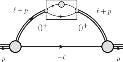
Figure C.2: Diagram 3: The probe interacts with the $0^{+}$ diquark within the proton and the dressed-quark is a bystander.

The vertex is given by ($\bar{N}=2$)

$$\mathcal{V}_{\mu}^{0}(P) =-\bar{e}_{0}\bar{N}\int\frac{d^{4}q}{(2\pi)^{4}}\,\text{tr}\Big{\{}S(q+P/2)\gamma_{\mu}S(q+P/2)$$

$$\quad\times\Gamma_{qq}^{0^{+}}(P)S(q-P/2)\bar{\Gamma}_{qq}^{0^{+}}(-P)\Big{\}}$$ (108)

$$=2\bar{e}_{0}\bar{N}\int_{0}^{1}dx\,(1-x)\int\frac{d^{4}q}{(2\pi)^{4}}\,$$

$$\quad\times\text{tr}\Big{\{}[i\gamma\cdot(q+xP)-M]\,\gamma_{\mu}\,[i\gamma\cdot(q+xP)-M]\,$$

$$\quad\times\gamma_{5}\Big{(}iE_{qq_{0}}+\frac{1}{M}\,\gamma\cdot P\,F_{qq_{0}}\Big{)}$$

$$\quad\times[i\gamma\cdot(q+(x-1)P)-M]\,$$

$$\quad\times\gamma_{5}\Big{(}iE_{qq_{0}}-\frac{1}{M}\,\gamma\cdot P\,F_{qq_{0}}\Big{)}\Big{\}}$$

$$\quad\times\Big{(}q^{2}-x(1-x)m_{qq_{0}}^{2}+M^{2}\Big{)}^{-3}\,,$$ (109)

where, again, $\bar{e}_{0}=\frac{1}{3}e$; and $P$ is the incoming as well as the outgoing momentum of the $0^{+}$ diquark, owing to our need to only consider vanishing momentum transfer $Q\to 0$, and we choose $P$ to be an on-shell momentum. Applying the projector in Eq. (101) and evaluating the trace, one obtains

$$eQ_{p,3} =D_{3}\,\bar{e}_{0}\,\mathcal{N}$$

$$=0.008733364\,\bar{e}_{0}\,\mathcal{N}=0.00291112\,e\,\mathcal{N}\,.$$ (110)

C.1.4 Diagram 4 – em

The fourth contribution is almost identical to that depicted in Fig. C.2: the only change being that in this instance the $1^{+}$ diquark is probed, so that one has

$$eQ_{p,4}\,\Lambda^{+}(p)\gamma_{\mu}\Lambda^{+}(p)$$

$$=\mathcal{N}\sum_{j\in 0,+}\Lambda^{+}(p)\,{\mathcal{A}}_{\alpha}^{j}(-p)\int\frac{d^{4}\ell}{(2\pi)^{4}}\,\Delta_{\alpha\alpha^{\prime}}^{1^{+}}(\ell+p)\mathcal{}$$

$$\quad\times V_{\alpha^{\prime}\mu\beta^{\prime}}^{j}(\ell+p)\Delta_{\beta^{\prime}\beta}^{1^{+}}(\ell+p)S(-\ell)\,\mathcal{A}_{\beta}^{j}(p)\,\Lambda^{+}(p)$$ (111)

$$=-2\,\mathcal{N}\sum_{j\in 0,+}\Lambda^{+}(p)\,\gamma_{5}\Big{(}a_{1}^{j}\gamma_{\alpha}+ia_{2}^{j}\hat{p}_{\alpha}\Big{)}\int_{0}^{1}dx\,(1-x)$$

$$\quad\times\int\frac{d^{4}\ell}{(2\pi)^{4}}\frac{i\gamma\cdot(-\ell+(1-x)p)-M}{[\ell^{2}-x(1-x)m_{N}^{2}+(1-x)m_{qq_{1}}^{2}+xM^{2}]^{3}}$$

$$\quad\times\mathbb{P}_{\alpha\alpha^{\prime}}(\ell+xp)\,\mathcal{V}_{\alpha^{\prime}\mu\beta^{\prime}}^{j}(\ell+xp)\,\mathbb{P}_{\beta^{\prime}\beta}(\ell+xp)$$

$$\quad\times\Big{(}a_{1}^{j}\gamma_{\beta}+ia_{2}^{j}\hat{p}_{\beta}\Big{)}\gamma_{5}\,\Lambda^{+}(p)\,.$$ (112)

The vertex is ($\bar{N}=2$)

$$\mathcal{V}_{\alpha\mu\beta}^{j} (P)=-\bar{e}_{j}\bar{N}\int\frac{d^{4}q}{(2\pi)^{4}}\,\text{tr}\Big{\{}S(q+P/2)\gamma_{\mu}S(q+P/2)$$

$$\quad\times\Gamma_{qq\beta}^{1^{+}}(P)S(q-P/2)\bar{\Gamma}_{qq\alpha}^{1^{+}}(-P)\Big{\}}$$ (113)

$$=-2\bar{e}_{j}\bar{N}E_{qq_{1}}^{2}\int_{0}^{1}dx\,(1-x)\int\frac{d^{4}q}{(2\pi)^{4}}\,$$

$$\quad\times\text{tr}\{[i\gamma\cdot(q+xP)-M]\,\gamma_{\mu}\,[i\gamma\cdot(q+xP)-M]\,$$

$$\quad\times\gamma_{\beta}^{T}(P)\,[i\gamma\cdot(q+(x-1)P)-M]\,\gamma_{\alpha}^{T}(P)\}$$

$$\quad\times[q^{2}-x(1-x)m_{qq_{1}}^{2}+M^{2}]^{-3}\,,$$ (114)

where, as noted above, $\bar{e}_{0}=\frac{1}{3}e$ and $\bar{e}_{+}=\frac{4}{3}e$, and $P$ is the incoming as well as outgoing momentum of the $1^{+}$ diquark. Applying the projector in Eq. (101) and evaluating the trace, one obtains

$$e Q_{p,4}=(2\,\bar{e}_{+}+\bar{e}_{0})\,D_{4}^{0}\,\mathcal{N}$$

$$=(2\,\bar{e}_{+}+\bar{e}_{0})\,0.00090133\,\mathcal{N}=0.002704\,e\,\mathcal{N}\,,$$ (115)

where $D_{4}^{0}$ is the contribution from the $\{ud\}$-diquark.

C.1.5 Diagram 5 – em

This contribution is depicted in Fig. C.3. In this case

$$Q_{p,5}e\,\Lambda^{+}(p)\gamma_{\mu}\Lambda^{+}(p)=0\,,$$ (116)

because the vertex vanishes at zero momentum transfer; i.e.,

$$\mathcal{V}_{\mu\alpha}=0\,.$$ (117)

Consequently

$$Q_{p,5}=0\,.$$ (118)

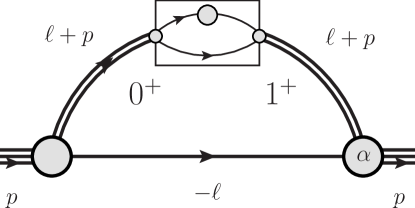
Figure C.3: Diagram 5: The probe is absorbed by a $0^{+}$-diquark, which is thereby transformed into a $1^{+}$ diquark.

C.1.6 Diagram 6 – em

This is the conjugate contribution to that depicted in Fig. C.3; namely, a $1^{+}$ diquark absorbs the probe and is thereby transformed into a $0^{+}$ diquark. In a symmetry preserving treatment of any reasonable interaction, this contribution is identical to that produced by Diagram 5.

C.1.7 Current Conservation

If a truly Poincaré invariant regularisation is employed, then one has Ward identities relating the charges in Eqs. (104), (115) and (105), (110)

$$D_{1}=D_{3}\,,\;D_{2}^{0}=D_{4}^{0}\,,$$ (119)

which ensure: simple additivity of the quark and diquark electric charges, and thereby guarantee a unit-charge isospin=$(+1/2)$ baryon through a single rescaling factor Oettel:1999gc ; and a neutral isospin=$(-1/2)$ baryon without fine tuning. Owing to the cutoffs we have introduced, however, these identities are violated: Eq. (104) cf. (110), Eq. (105) cf. (115). Following Ref. Wilson:2011aa , we ameliorate this flaw by enforcing the Ward identities:

$$D_{1,3} \to D_{\overline{13}}=(D_{1}+D_{3})/2=0.01350\,,\;$$ (120a)

$$D_{2,4} \to D_{\overline{24}}=3(D_{2}^{0}+D_{4}^{0})/2=0.00429\,.$$ (120b)

This corresponds to introducing a rescaling factor for each of the diagrams involved: $D_{i}\to\kappa_{i}D_{i}$, $\kappa_{1,3}=D_{\overline{13}}/D_{1,3}$, $\kappa_{2,4}=D_{\overline{24}}/D_{2,4}$. Diagrams 5 and 6 are unaffected because they are equal and do not contribute to a baryon’s charge.

C.1.8 Canonical Normalisation

The results computed from all diagrams considered in connection with the proton’s charge are collected in Table C.1. As noted above, the canonical normalisation is fixed by requiring

$$Q_{p}=\sum_{i=1}^{6}\,Q_{p,i}=1\,,$$ (121)

from which it follows that

$$\mathcal{N}=\frac{1}{0.01777}=56.27\,.$$ (122)

	$Q_{p,i}/\mathcal{N}$	$Q^{\kappa}_{p,i}/\mathcal{N}$
Diagram 1	$0.01217$	0.0090
Diagram 2	$0$	0
Diagram 3	$0.00291$	$0.00450$
Diagram 4	$0.00270$	$0.00426$
Diagram 5	$0$
Diagram 6	$0$
Sum	$0.0178$	$0.0178$

Table C.1: Column 1: Summary of the results computed from all diagrams considered in connection with the proton’s charge. Column 2: Results scaled as described in Sec. C.1.7.

C.2 Scalar Current

When computing the scalar charge of any hadron, one must employ the dressed-quark-scalar vertex. That vertex, too, is obtained by solving an inhomogeneous Bethe-Salpeter equation: in this case, the unrenormalised form is determined by the inhomogeneous term ${\mathbb{1}}$. The complete solution for the contact-interaction’s scalar vertex in RL truncation can be found in Refs. Chen:2012txa , and at $Q^{2}=0$ this yields:

$$\mathcal{V}^{q}_{\mathbb{1}}=\frac{1}{\displaystyle 1+\frac{4\alpha_{\text{IR}}}{3\pi m_{G}^{2}}\Big{(}2\,\mathcal{C}_{1}^{\text{iu}}(M^{2})-\mathcal{C}^{\text{iu}}(M^{2})\Big{)}}\,{\mathbb{1}}=1.37\,{\mathbb{1}}\,,$$ (123)

where $M$ is the dressed-quark mass in Eq. (52).

As a check on this result, we note again that since the vertex is only required at $Q^{2}=0$, one can appeal to a Ward identity Chang:2008ec , which takes the form

$${\mathcal{V}}_{\mathbb{1}}(Q)\stackrel{{\scriptstyle Q^{2}=0}}{{=}}{\mathbb{1}}\,\frac{\partial M}{\partial m}\,$$ (124)

when the contact interaction is used. Employing the results from which Ref. Roberts:2011cf was prepared, this expression, too, yields the numerical value in Eq. (123).

The nucleon’s scalar charge is also known as the nucleon $\sigma$-term; and using our implementation of the contact interaction, one need consider only relevant analogues of the six diagrams described explicitly in App. C.1. In this case, Diagrams 1–4 provide a nonzero contribution and the complete result is obtained from the sum.

C.2.1 Diagram 1 – scalar

This is the contribution produced by the scalar probe interacting with a the dressed-quark whilst the $0^{+}$ $[ud]$-diquark is a spectator:

$$\hat{\sigma}_{q,1} \,\Lambda^{+}(p){\mathbb{1}}\Lambda^{+}(p)={\mathcal{N}}_{1}^{\kappa}\,\Lambda^{+}(p)\,\bar{\,\mathcal{S}\,}\int\frac{d^{4}\ell}{(2\pi)^{4}}\,S(\ell+p)$$

$$\quad\times\mathcal{V}^{q}_{\mathbb{1}}S(\ell+p)\Delta^{0^{+}}(-\ell)\,\mathcal{S}\,\Lambda^{+}(p)$$ (125)

$$=2\,{\mathcal{N}}_{1}^{\kappa}\,\Lambda^{+}(p)\,s^{2}\int_{0}^{1}dx\,(1-x)\int\frac{d^{4}\ell}{(2\pi)^{4}}$$

$$\;\times\frac{\{i\gamma\cdot(\ell+xp)-M\}\,\mathcal{V}_{\mathbb{1}}^{q}\,\{i\gamma\cdot(\ell+xp)-M\}}{[\ell^{2}-x(1-x)m_{N}^{2}+(1-x)M^{2}+xm_{qq_{0}}^{2}]^{3}}\,\Lambda^{+}(p)\,,$$ (126)

where ${\mathcal{N}}_{1}^{\kappa}=\kappa_{1}{\mathcal{N}}$, with $\kappa_{1}$ defined in connection with Eqs. (120), ${\mathcal{N}}$ given in Eq. (122). Applying the projector

$$\mathcal{P}=\frac{1}{2}\,{\mathbb{1}}\,,$$ (127)

and evaluating the trace, one obtains

$$\hat{\sigma}_{u,1}=\hat{\sigma}_{q,1}=0.309\,,\;\hat{\sigma}_{d,1}=0\,.$$ (128)

It was plain from the outset that this diagram would only produce a contribution to $\hat{\sigma}_{u,1}$ because the $d$-quark is sequestered inside the scalar diquark.

C.2.2 Diagram 2 – scalar

In this case we have the scalar probe interacting with the dressed-quark and the $1^{+}$ diquarks being spectators:

$$\hat{\sigma}_{q_{j,2}}\,\Lambda^{+}(p){\mathbb{1}}\Lambda^{+}(p)$$

$$={\mathcal{N}}_{2}^{\kappa}\,\Lambda^{+}(p)\,{\mathcal{A}}_{\alpha}^{j}(-p)\int\frac{d^{4}\ell}{(2\pi)^{4}}\,S(\ell+p)\mathcal{V}^{q}_{\mathbb{1}}$$

$$\quad\times S(\ell+p)\Delta_{\alpha\beta}^{1^{+}}(-\ell)\,\mathcal{A}_{\beta}^{j}(p)\,\Lambda^{+}(p)$$ (129)

$$=2\,{\mathcal{N}}_{2}^{\kappa}\,\Lambda^{+}(p)\,\gamma_{5}\Big{(}a_{1}^{j}\gamma_{\alpha}+ia_{2}^{j}\hat{p}_{\alpha}\Big{)}\!\!\int_{0}^{1}dx\,(1-x)\!\!\int\frac{d^{4}\ell}{(2\pi)^{4}}$$

$$\quad\times\frac{\{i\gamma\cdot(\ell+xp)-M\}\,\mathcal{V}^{q}_{\mathbb{1}}\,\{i\gamma\cdot(\ell+xp)-M\}}{[\ell^{2}-x(1-x)m_{N}^{2}+(1-x)M^{2}+xm_{qq^{1}}^{2}]^{3}}$$

$$\quad\times\mathbb{P}_{\alpha\beta}(\ell-(1-x)p)\!\Big{(}a_{1}^{j}\gamma_{\beta}+ia_{2}^{j}\hat{p}_{\beta}\Big{)}\gamma_{5}\,\Lambda^{+}(p).$$ (130)

Applying the projector in Eq. (127) and evaluating the trace, one finds, owing to Eq. (88),

$$\hat{\sigma}_{u,2}=\hat{\sigma}_{q_{0,2}}=0.0318\,,\;\hat{\sigma}_{d,2}=\hat{\sigma}_{q_{+,2}}=0.0636=2\hat{\sigma}_{u,2}\,.$$ (131)

C.2.3 Diagram 3 – scalar

The third diagram describes the scalar probe interacting with the $0^{+}$ $[ud]$-diquark and the dressed-quark acting merely as an onlooker:

$$\hat{\sigma}_{q,3}\,\Lambda^{+}(p){\mathbb{1}}\Lambda^{+}(p)={\mathcal{N}}_{3}^{\kappa}\,\Lambda^{+}(p)\,\bar{\,\mathcal{S}\,}\int\frac{d^{4}\ell}{(2\pi)^{4}}\,\Delta^{0^{+}}(\ell+p)$$

$$\quad\times\mathcal{V}_{\mathbb{1}}^{0}(\ell+p)\Delta^{0^{+}}(\ell+p)S(-\ell)\,\mathcal{S}\,\Lambda^{+}(p)$$ (132)

$$=-2\,{\mathcal{N}}_{3}^{\kappa}\,s^{2}\int_{0}^{1}dx\,(1-x)\int\frac{d^{4}\ell}{(2\pi)^{4}}\Lambda^{+}(p)$$

$$\times\frac{[i\gamma\cdot(-\ell+(1-x)p)-M]\mathcal{V}^{0}_{\mathbb{1}}(\ell+xp)\,\Lambda^{+}(p)}{[\ell^{2}-x(1-x)m_{N}^{2}+(1-x)m_{qq^{0}}^{2}+xM^{2}]^{3}}\,.$$ (133)

The vertex is given by ($\bar{N}=2$)

$$\mathcal{V}^{0}_{\mathbb{1}}(P)=-2\bar{N}\int\frac{d^{4}q}{(2\pi)^{4}}\,\text{tr}\Big{\{}S(q+P/2)\mathcal{V}^{q}_{\mathbb{1}}S(q+P/2)$$

$$\quad\times\Gamma_{qq}^{0^{+}}(P)S(q-P/2)\bar{\Gamma}_{qq}^{0^{+}}(-P)\Big{\}}$$ (134)

$$=4\bar{N}\int_{0}^{1}dx\,(1-x)\int\frac{d^{4}q}{(2\pi)^{4}}\,\text{tr}\Big{\{}[i\gamma\cdot(q+xP)-M]\,$$

$$\quad\times\mathcal{V}^{q}_{\mathbb{1}}\,[i\gamma\cdot(q+xP)-M]\,\gamma_{5}\Big{(}iE_{qq_{0}}+\frac{1}{M}\,\gamma\cdot P\,F_{qq_{0}}\Big{)}$$

$$\quad\times[i\gamma\cdot(q+(x-1)P)-M]\,\gamma_{5}\Big{(}iE_{qq_{0}}$$

$$\quad-\frac{1}{M}\,\gamma\cdot P\,F_{qq_{0}}\Big{)}\Big{\}}\Big{(}q^{2}-x(1-x)m_{qq_{0}}^{2}+M^{2}\Big{)}^{-3}\,.$$ (135)

Applying the projector in Eq. (127) and evaluating the trace, one obtains

$$\hat{\sigma}_{u,3}=\frac{\hat{\sigma}_{q,3}}{2}=1.0419=\hat{\sigma}_{d,3}\,.$$ (136)

C.2.4 Diagram 4 – scalar

The fourth diagram describes the scalar probe interacting with a $1^{+}$ $\{uu\}$- or $\{ud\}$-diquark where the dressed-quark acts merely as an onlooker:

$$\hat{\sigma}_{q_{j,4}}\,\Lambda^{+}(p){\mathbb{1}}\Lambda^{+}(p)$$

$$={\mathcal{N}}_{4}^{\kappa}\,\Lambda^{+}(p)\,{\mathcal{A}}_{\alpha}^{j}(-p)\int\frac{d^{4}\ell}{(2\pi)^{4}}\,\Delta_{\alpha\alpha^{\prime}}^{1^{+}}(\ell+p)\mathcal{V}_{\alpha^{\prime}\beta^{\prime}}^{\mathbb{1}}(\ell+p)$$

$$\quad\times\Delta_{\beta^{\prime}\beta}^{1^{+}}(\ell+p)S(-\ell)\,\mathcal{A}_{\beta}^{j}(p)\,\Lambda^{+}(p)$$ (137)

$$=-2\,{\mathcal{N}}_{4}^{\kappa}\,\Lambda^{+}(p)\,\gamma_{5}\Big{(}a_{1}^{j}\gamma_{\alpha}+ia_{2}^{j}\hat{p}_{\alpha}\Big{)}\int_{0}^{1}dx\,(1-x)$$

$$\quad\times\int\frac{d^{4}\ell}{(2\pi)^{4}}\frac{i\gamma\cdot(-\ell+(1-x)p)-M}{[\ell^{2}-x(1-x)m_{N}^{2}+(1-x)m_{qq_{1}}^{2}+xM^{2}]^{3}}$$

$$\quad\times\mathbb{P}_{\alpha\alpha^{\prime}}(\ell+xp)\,\mathcal{V}^{\mathbb{1}}_{\alpha^{\prime}\beta^{\prime}}(\ell+xp)\,\mathbb{P}_{\beta^{\prime}\beta}(\ell+xp)$$

$$\quad\times\Big{(}a_{1}^{j}\gamma_{\beta}+ia_{2}^{j}\hat{p}_{\beta}\Big{)}\gamma_{5}\,\Lambda^{+}(p)\,.$$ (138)

The vertex is given by ($\bar{N}=2$)

$$\mathcal{V}^{\mathbb{1}}_{\alpha\beta}(P)=-2\bar{N}\int\frac{d^{4}q}{(2\pi)^{4}}\,\text{tr}\Big{\{}S(q+P/2)\mathcal{V}_{\mathbb{1}}^{q}S(q+P/2)$$

$$\quad\times\Gamma_{qq\beta}^{1^{+}}(P)S(q-P/2)\bar{\Gamma}^{1^{+}}_{qq\alpha}(-P)\Big{\}}$$ (139)

$$=-4\bar{N}E_{qq_{1}}^{2}\int_{0}^{1}dx\,(1-x)\int\frac{d^{4}q}{(2\pi)^{4}}\,\text{tr}\{[i\gamma\cdot(q+xP)$$

$$\quad-M]\,\mathcal{V}^{q}_{\mathbb{1}}\,[i\gamma\cdot(q+xP)-M]\,\gamma_{\beta}^{T}\,[i\gamma\cdot(q+(x-1)P)$$

$$\quad-M]\,\gamma_{\alpha}^{T}\}[q^{2}-x(1-x)m_{qq_{1}}^{2}+M^{2}]^{-3}$$ (140)

$$\to 16M\bar{N}E_{qq_{1}}^{2}\mathcal{V}^{q}_{\mathbb{1}}\mathbb{P}_{\alpha\beta}(P)\int_{0}^{1}dx\,(1-x)$$

$$\quad\times\Big{(}M^{2}-x(x-2)m_{qq_{1}}^{2}\Big{)}\,\mathcal{G}_{1}^{\rm iu}\Big{(}x(x-1)m_{qq_{1}}^{2}+M^{2}\Big{)}\,,$$ (141)

where $P$ is again both the incoming and outgoing momentum of the $1^{+}$ diquark.

Applying the projector in Eq. (127) and evaluating the trace, one finds

$$\hat{\sigma}_{u,4}=\frac{\hat{\sigma}_{q_{0,4}}}{2}+\hat{\sigma}_{q_{+,4}}=0.465\,,\;\hat{\sigma}_{d,4}=\frac{\hat{\sigma}_{q_{0,4}}}{2}=0.0938\,.$$ (142)

C.2.5 Proton $\mathbf{\sigma}$-term

The results obtained from all diagrams considered in connection with the proton’s scalar charge are collected in Table C.2. The proton $\sigma$-term is

$$\sigma_{N}=m\sum_{i=1}^{6}[\hat{\sigma}_{u,i}+\hat{\sigma}_{d,i}]=21.33\,{\rm MeV}.$$ (143)

In the isospin symmetric limit, the neutron $\sigma$-term is identical.

	$\hat{\sigma}_{u}$	$\hat{\sigma}_{d}$	$\sigma$ [MeV]
Diagram 1	$0.309$	$0$	$\phantom{1}2.163$
Diagram 2	$0.032$	$0.063$	$\phantom{1}0.666$
Diagram 3	$1.042$	$1.042$	$14.587$
Diagram 4	$0.465$	$0.094$	$\phantom{1}3.914$
Diagram 5	$0$	$0$	$\phantom{1}0$
Diagram 6	$0$	$0$	$\phantom{1}0$
Total Result	$1.85$	$1.20$	$21.33$

Table C.2: Summary of the results computed from all diagrams considered in connection with the proton’s scalar charge.

C.3 Tensor Current

When computing the tensor charge of any hadron, one must employ the dressed-quark-tensor vertex. However, as explained elsewhere Roberts:2011cf , any dressing of the tensor vertex must depend linearly on the relative momentum LlewellynSmith:1969az and such dependence is impossible using a symmetry-preserving regularisation of a vector$\,\otimes\,$vector contact interaction. Hence, in our case, the quark-tensor vertex is unmodified from its bare form; viz.,

$$\mathcal{V}_{\mu\nu}^{q}=\sigma_{\mu\nu}\,.$$ (144)

Naturally, when computing the proton’s tensor charge using our implementation of the contact interaction, one need only consider relevant analogues of the six diagrams described explicitly in App. C.1. In this case, Diagrams 1,2,4,5,6 provide nonzero contributions. Diagram 3 yields zero because Poincaré invariance entails that a scalar diquark cannot possess a tensor charge.

C.3.1 Diagram 1 – tensor

As usual, we first consider the case of the tensor probe interacting with the dressed-quark and the $0^{+}$ $[ud]$-diquark being a spectator:

$$\delta_{1}q \,\Lambda^{+}(p)\sigma_{\mu\nu}\Lambda^{+}(p)={\mathcal{N}}_{1}^{\kappa}\,\Lambda^{+}(p)\,\bar{\,\mathcal{S}\,}\int\frac{d^{4}\ell}{(2\pi)^{4}}\,S(\ell+p)\sigma_{\mu\nu}$$

$$\quad\times S(\ell+p)\Delta^{0^{+}}(-\ell)\,\mathcal{S}\,\Lambda^{+}(p)$$ (145)

$$=2\,\mathcal{N}\,s^{2}\int_{0}^{1}dx\,(1-x)\int\frac{d^{4}\ell}{(2\pi)^{4}}\Lambda^{+}(p)\,\{i\gamma\cdot(\ell+xp)$$

$$\quad-M\}\,\sigma_{\mu\nu}\,\{i\gamma\cdot(\ell+xp)-M\}\Lambda^{+}(p)\,$$

$$\quad\times[\ell^{2}-x(1-x)m_{N}^{2}+(1-x)M^{2}+xm_{qq_{0}}^{2}]^{-3}\,.$$ (146)

Applying the projector

$$\mathcal{P}_{\mu\nu}=\frac{1}{12}\,\sigma_{\mu\nu}\,,$$ (147)

and evaluating the trace, one obtains

$$\delta_{1}q =2\,{\mathcal{N}}_{1}\,s^{2}\int_{0}^{1}dx\,(1-x)\int\frac{d^{4}\ell}{(2\pi)^{4}}$$

$$\quad\times\frac{(M+xm_{N})^{2}}{[\ell^{2}-x(1-x)m_{N}^{2}+(1-x)M^{2}+xm_{qq_{0}}^{2}]^{3}}$$ (148)

$$\to 2\,\mathcal{N}\,s^{2}\int_{0}^{1}dx\,(1-x)(M+xm_{N})^{2}\,$$

$$\quad\times\mathcal{G}_{1}^{\rm iu}\Big{(}x(x-1)m_{N}^{2}+(1-x)M^{2}+xm_{qq_{0}}^{2}\Big{)}\,,$$ (149)

where $\mathcal{G}_{1}^{\rm iu}(\omega)$ is defined in Eq. (46). As a result we find

$$\delta_{T1}u=\delta_{1}q=0.581\,,\quad\delta_{T1}d=0\,.$$ (150)

C.3.2 Diagram 2 – tensor

When the tensor probe interacts with the dressed-quark and the $1^{+}$ diquarks are spectators, one has

$$\delta_{2}q_{j}\,\Lambda^{+}(p)\sigma_{\mu\nu}\Lambda^{+}(p)$$

$$={\mathcal{N}}_{2}^{\kappa}\,\Lambda^{+}(p)\,{\mathcal{A}}_{\alpha}^{j}(-p)\int\frac{d^{4}\ell}{(2\pi)^{4}}\,S(\ell+p)\sigma_{\mu\nu}$$

$$\quad\times S(\ell+p)\,\Delta_{\alpha\beta}^{1^{+}}(-\ell)\,\mathcal{A}_{\beta}^{j}(p)\,\Lambda^{+}(p)$$ (151)

$$=2\,{\mathcal{N}}_{2}^{\kappa}\,\Lambda^{+}(p)\,\gamma_{5}\Big{(}a_{1}^{j}\gamma_{\alpha}+ia_{2}^{j}\hat{p}_{\alpha}\Big{)}\int_{0}^{1}dx\,(1-x)\int\frac{d^{4}\ell}{(2\pi)^{4}}$$

$$\quad\times\frac{\{i\gamma\cdot(\ell+xp)-M\}\,\sigma_{\mu\nu}\,\{i\gamma\cdot(\ell+xp)-M\}}{[\ell^{2}-x(1-x)m_{N}^{2}+(1-x)M^{2}+xm_{qq_{1}}^{2}]^{3}}$$

$$\quad\times\mathbb{P}_{\alpha\beta}(\ell-(1-x)p)\Big{(}a_{1}^{j}\gamma_{\beta}+ia_{2}^{j}\hat{p}_{\beta}\Big{)}\gamma_{5}\Lambda^{+}(p).$$ (152)

Applying the projector in Eq. (147) and evaluating the resulting trace, one finds, owing to Eq. (88):

$$\delta_{T2}d=\delta_{2}q_{+}=2\delta_{2}q_{0}=-0.0359=2\delta_{T2}u\,.$$ (153)

C.3.3 Diagram 4 – tensor

The next nonzero contribution arises from the tensor probe interacting with a $1^{+}$ $\{uu\}$- or $\{ud\}$-diquark where the dressed-quark acts merely as an onlooker:

$$\delta_{4}q_{j}\,\Lambda^{+}(p)\sigma_{\mu\nu}\Lambda^{+}(p)$$

$$={\mathcal{N}}_{4}^{\kappa}\,\Lambda^{+}(p)\,{\mathcal{A}}_{\alpha}^{j}(-p)\int\frac{d^{4}\ell}{(2\pi)^{4}}\,\Delta_{\alpha\alpha^{\prime}}^{1^{+}}(\ell+p)\mathcal{V}^{2}_{\alpha^{\prime}\mu\nu\beta^{\prime}}(\ell+p)$$

$$\quad\times\Delta_{\beta^{\prime}\beta}^{1^{+}}(\ell+p)S(-\ell)\,\mathcal{A}_{\beta}^{j}(p)\,\Lambda^{+}(p)$$ (154)

$$=-2\,{\mathcal{N}}_{4}^{\kappa}\,\Lambda^{+}(p)\,\gamma_{5}\Big{(}a_{1}^{j}\gamma_{\alpha}+ia_{2}^{j}\hat{p}_{\alpha}\Big{)}\int_{0}^{1}dx\,(1-x)\int\frac{d^{4}\ell}{(2\pi)^{4}}$$

$$\quad\times\frac{i\gamma\cdot(-\ell+(1-x)p)-M}{[\ell^{2}-x(1-x)m_{N}^{2}+(1-x)m_{qq_{1}}^{2}+xM^{2}]^{3}}$$

$$\quad\times\mathbb{P}_{\alpha\alpha^{\prime}}(\ell+xp)\,\mathcal{V}^{2}_{\alpha^{\prime}\mu\nu\beta^{\prime}}(\ell+xp)\,$$

$$\quad\times\mathbb{P}_{\beta^{\prime}\beta}(\ell+xp)\Big{(}a_{1}^{j}\gamma_{\beta}+ia_{2}^{j}\hat{p}_{\beta}\Big{)}\gamma_{5}\,\Lambda^{+}(p)\,.$$ (155)

The vertex is ($\bar{N}=2$)

$$\mathcal{V}^{2}_{\alpha\mu\nu\beta}(P)=-2\bar{N}\int\frac{d^{4}q}{(2\pi)^{4}}\,\text{tr}\Big{\{}S(q+P/2)\sigma_{\mu\nu}S(q+P/2)$$

$$\quad\times\Gamma_{qq\beta}^{1^{+}}(P)S(q-P/2)\bar{\Gamma}_{qq\alpha}^{1^{+}}(-P)\Big{\}}$$ (156)

$$=-4\bar{N}E_{qq_{1}}^{2}\int_{0}^{1}dx\,(1-x)\int\frac{d^{4}q}{(2\pi)^{4}}\,\text{tr}\bigg{[}[i\gamma\cdot(q+xP)$$

$$\quad-M]\,\sigma_{\mu\nu}\,[i\gamma\cdot(q+xP)-M]\,\gamma_{\beta}^{T}\,$$

$$\quad\times[i\gamma\cdot(q+(x-1)P)-M]\,\gamma_{\alpha}^{T}\bigg{]}$$

$$\quad\times[q^{2}-x(1-x)m_{qq_{1}}^{2}+M^{2}]^{-3}$$ (157)

$$\to 16iM\bar{N}E_{qq_{1}}^{2}\Big{(}\mathbb{P}_{\alpha\mu}(P)\mathbb{P}_{\beta\nu}(P)-\mathbb{P}_{\alpha\nu}(P)\mathbb{P}_{\beta\mu}(P)\Big{)}$$

$$\quad\times\int_{0}^{1}dx\,(1-x)\Big{\{}\Big{(}M^{2}-x(x-2)m_{qq_{1}}^{2}\Big{)}\,\mathcal{G}_{1}^{\rm iu}(\omega)$$

$$\quad+\mathcal{G}_{2}^{\rm iu}\Big{(}x(x-1)m_{qq_{1}}^{2}+M^{2}\Big{)}\Big{\}}$$ (158)

where $P$ is the incoming and outgoing momentum of the $1^{+}$ diquark, and $\mathcal{G}_{1}^{\rm iu}(\omega)$, $\mathcal{G}_{2}^{\rm iu}(\omega)$ are defined in Eqs. (46), (A). Applying the projector in Eq. (147) and evaluating the resulting trace, one finds

$$\delta_{T4}u=\frac{\delta_{4}q_{0}}{2}+\delta_{4}q_{+}=0.292\,,\;\delta_{T4}d=\frac{\delta_{4}q_{0}}{2}=0.0589\,.$$ (159)

C.3.4 Diagram 5 – tensor

This is the contribution to the tensor charge arising when a scalar diquark absorbs the tensor probe and is thereby transformed into a $1^{+}$ diquark. Naturally, in a symmetry preserving treatment of any reasonable interaction, this contribution is identical to that produced by Diagram 6. Concretely, one has:

$$\delta_{5}q\,\Lambda^{+}(p)\sigma_{\mu\nu}\Lambda^{+}(p)$$

$$={\mathcal{N}}_{5}^{\kappa}\,\Lambda^{+}(p)\,{\mathcal{A}}_{\alpha}^{0}(-p)\int\frac{d^{4}\ell}{(2\pi)^{4}}\,\Delta_{\alpha\beta}^{1^{+}}(\ell+p)\mathcal{V}^{10}_{\beta\mu\nu}(\ell+p)$$

$$\quad\times\Delta^{0^{+}}(\ell+p)S(-\ell)\,\mathcal{S}\,\Lambda^{+}(p)$$ (160)

$$=-2\,{\mathcal{N}}_{5}^{\kappa}\,\Lambda^{+}(p)\,\gamma_{5}\Big{(}a_{1}^{0}\gamma_{\alpha}+ia_{2}^{0}\hat{p}_{\alpha}\Big{)}\int_{0}^{1}dx\int_{0}^{1}dy\,y\int\frac{d^{4}\ell}{(2\pi)^{4}}$$

$$\quad\times[i\gamma\cdot(-\ell+yp)-M]\mathcal{V}^{10}_{\beta\mu\nu}(\ell+(1-y)p)\,$$

$$\quad\times\mathbb{P}_{\alpha\beta}(\ell+(1-y)p)\,s\,\Lambda^{+}(p)[\ell^{2}+y(y-1)m_{N}^{2}$$

$$\quad+xym_{qq_{1}}^{2}+(1-x)ym_{qq_{0}}^{2}+(1-y)M^{2}]^{-3}\,.$$ (161)

The transition vertex is $\mathcal{V}^{10}_{\beta\mu\nu}(P,P)$ where ($\bar{N}=2$)

$$\mathcal{V}^{10}_{\beta\mu\nu}(P,P^{\prime})=-2\bar{N}\int\frac{d^{4}q}{(2\pi)^{4}}\,\text{tr}\Big{\{}S(q+P^{\prime})\sigma_{\mu\nu}S(q+P)$$

$$\quad\times\Gamma_{qq}^{0^{+}}(P)S(q)\bar{\Gamma}_{qq\beta}^{1^{+}}(-P^{\prime})\Big{\}}$$ (162)

$$=4i\bar{N}E_{qq_{1}}\int_{0}^{1}dx\int_{0}^{1}dy\,y\int\frac{d^{4}q}{(2\pi)^{4}}\,$$

$$\quad\times\text{tr}\Big{\{}[i\gamma\cdot(q+yP^{\prime}-xyP)-M]\,\sigma_{\mu\nu}\,$$

$$\quad\times[i\gamma\cdot(q-(1-y)P^{\prime}+(1-xy)P)-M]$$

$$\quad\times\gamma_{5}\Big{(}iE_{qq_{0}}+\frac{1}{M}\,\gamma\cdot P\,F_{qq_{0}}\Big{)}\,$$

$$\quad\times[i\gamma\cdot(q-(1-y)P^{\prime}-xyP)-M]\,\gamma_{\beta}^{T}(P^{\prime})\Big{\}}$$

$$\quad\times\Big{(}q^{2}-(1-x)y(1-y)m_{qq_{1}}^{2}$$

$$\quad\quad-x(1-x)y^{2}m_{qq_{0}}^{2}+M^{2}\Big{)}^{-3},$$ (163)

where $P$ and $P^{\prime}$ are the incoming and outgoing momenta of the diquarks, respectively. (Some details about the on-shell procedure can be found in App. D.) Applying the projector in Eq. (147), evaluating the resulting trace and combining the result with that from Diagram 6, one finds

$$\delta_{T,{5+6}}u=\delta_{T,{5+6}}d=\delta q_{5}=-0.164\,.$$ (164)

C.3.5 Proton tensor charge

The results obtained from all diagrams considered in connection with the proton’s tensor charges are collected in Table C.3. Notably, the values of the tensor charges depend on the renormalisation scale associated with the tensor vertex. This is discussed in App. F.

	$\delta_{T}u$	$\delta_{T}d$	$g_{T}^{(0)}$	$g_{T}^{(1)}$
Diagram 1	$\phantom{-}0.581$	$0$	$\phantom{-}0.581$	$0.581$
Diagram 2	$-0.018$	$-0.036$	$-0.054$	$0.018$
Diagram 3	$\phantom{-}0$	$0$	$\phantom{-}0$	$0$
Diagram 4	$\phantom{-}0.292$	$\phantom{-}0.059$	$\phantom{-}0.351$	$0.233$
Diagram 5+6	$-0.164$	$-0.164$	$-0.329$	$0$
Total Result	$\phantom{-}0.691$	$-0.141$	$\phantom{-}0.550$	$0.832$

Table C.3: Summary of results computed from all diagrams considered in connection with the proton’s tensor charge. They represent values at the model scale, $\zeta_{H}\approx M$, described in App. E.

C.3.6 Proton tensor charge – scalar diquark only

It is interesting to consider the impact of the axial-vector diquark on the tensor charges. This may be exposed by comparing the results in Table C.3 with those obtained when the axial-vector diquark is eliminated from the nucleon. We implement that suppression by using the following nucleon Faddeev amplitude:

$$\begin{array}[]{ccccc}s(P)&a_{1}^{+}(P)&a_{1}^{0}(P)&a_{2}^{+}(P)&a_{2}^{0}(P)\\ 1.0&0&0&0&0\end{array}\,,$$ (165)

and then repeating the computations in Apps. C.1, C.3. Naturally, in this case only Diagrams 1 and 3 can possibly yield nonzero contributions to any quantity.

Recomputing the canonical normalisation, we obtain

$$\mathcal{N}_{\not\,1}=\frac{1}{0.0174}=57.50\,,$$ (166)

which is 2% larger than the complete result in Eq. (122).

Regarding the tensor charges, Diagram 3 also vanishes in this instance so that the net result is simply that produced by Diagram 1:

$$\begin{array}[]{cccc}\delta_{T\!\not\,1}u&\delta_{T\!\not\,1}d&g_{T\!\not\,1}^{(0)}&g_{T\!\not\,1}^{(1)}\\ 0.765&0&0.765&0.765\end{array}\,.$$ (167)

Comparison with Table C.3 shows that with a symmetry-preserving treatment of a vector$\,\otimes\,$vector contact interaction, the $d$-quark contribution to the proton’s tensor charge is only nonzero in the presence of axial-vector diquark correlations and these correlations reduce the $u$-quark contribution by 10%.

C.3.7 Proton tensor charge – Reduced DCSB

In order to expose the effect of DCSB on the tensor charges, we repeated all relevant calculations above beginning with the value of $\alpha_{\rm IR}$ used to produce Eq. (53) and thereby obtained the results listed in Table C.4.

	$\delta_{T}u$	$\delta_{T}d$	$g_{T}^{(0)}$	$g_{T}^{(1)}$
Diagram 1	$\phantom{-}0.495$	$0$	$\phantom{-}0.495$	$0.495$
Diagram 2	$-0.020$	$-0.039$	$-0.059$	$0.020$
Diagram 3	$\phantom{-}0$	$0$	$\phantom{-}0$	$0$
Diagram 4	$\phantom{-}0.236$	$\phantom{-}0.047$	$\phantom{-}0.283$	$0.189$
Diagram 5+6	$-0.160$	$-0.160$	$-0.319$	$0$
Total Result	$\phantom{-}0.551$	$-0.151$	$\phantom{-}0.400$	$0.703$

Table C.4: Summary of results computed from all diagrams considered in connection with the proton’s tensor charge using input based on $\alpha_{\rm IR}/\pi=0.74$, quoted at the model scale, $\zeta_{H}\approx M$, described in App. E.

Appendix D On-shell Considerations for the Transition Diagrams

For the practitioner it will likely be helpful here to describe our treatment of the denominator that arises when using a Feynman parametrisation to compute the transition diagrams. Namely, one has

$$\frac{1}{(q+P^{\prime})^{2}+M^{2}}\frac{1}{(q+P)^{2}+M^{2}}\frac{1}{q^{2}+M^{2}}$$

$$=2\int_{0}^{1}dx\int_{0}^{1}dy\,y\{(q+(1-y)P^{\prime}+xyP)^{2}$$

$$\quad+(1-y)yP^{\prime 2}+xy(1-xy)P^{2}$$

$$\quad-2(1-y)xyP^{\prime}\cdot P+M^{2}\}^{-3}\,.$$ (168)

At this point, a shift of the integration variable $q\to q-(1-y)P^{\prime}-xyP$ yields

$$2\int_{0}^{1}dx\int_{0}^{1}dy\,y\{q^{2}+(1-y)yP^{\prime 2}+xy(1-xy)P^{2}$$

$$\quad-2(1-y)xyP^{\prime}\cdot P+M^{2}\}^{-3}\,.$$ (169)

Next, we employ on-shell relations, which for Diagram 5 are given by

$$P^{\prime 2}=-m_{qq_{1}}^{2}\,,\;P^{2}=-m_{qq_{0}}^{2}\,.$$ (170)

Then, since $Q^{2}\equiv(P^{\prime}-P)^{2}=P^{\prime 2}+P^{2}-2P^{\prime}\cdot P=0$:

$$P^{\prime}\cdot P=-\frac{m_{qq_{0}}^{2}+m_{qq_{1}}^{2}}{2}\,.$$ (171)

Hence, the Feynman integral associated with Diagram 5 is

$$2\int_{0}^{1}dx\int_{0}^{1}dy\,y\{q^{2}-(1-x)y(1-y)m_{qq_{1}}^{2}$$

$$\quad-x(1-x)y^{2}m_{qq_{0}}^{2}+M^{2}\}^{-3}\,.$$ (172)

Diagram 6 is obtained via $m_{qq_{0}}\leftrightarrow m_{qq_{1}}$.

Appendix E Model Scale

In modern studies of QCD’s gap equation, which use DCSB-improved kernels and interactions that preserve the one-loop renormalisation group behaviour of QCD, the dressed-quark mass is renormalisation point invariant. As in QCD, however, the current-quark mass is not. Therefore, in quoting a current-quark mass in Eq. (51), a question immediately arises: to which scale, $\zeta_{H}$, does this current-quark mass correspond?

As noted in App. A, the contact-interaction does not define a renormalisable theory and the scale $\zeta_{H}$ should therefore be part of the definition of the interaction. We define $\zeta_{H}$ so as to establish contact between the current-quark mass in Eq. (51) and QCD.

Current-quark masses in QCD are typically quoted at a scale of $\zeta_{2}=2\,$GeV. A survey of available estimates indicates Beringer:1900zz

$$m(\zeta_{2})=\frac{m_{u}(\zeta_{2})+m_{d}(\zeta_{2})}{2}=3.5^{+0.7}_{-0.2}\,;$$ (173)

and this value compares well with that determined from a compilation of estimates using numerical simulations of lattice-regularised QCD Colangelo:2010et :

$$m(\zeta_{2})=\frac{m_{u}(\zeta_{2})+m_{d}(\zeta_{2})}{2}=3.4\pm 0.2\,.$$ (174)

On the other hand, we have determined an average value of the $u$- and $d$-quark masses appropriate to our interaction that is $m(\zeta_{H}):=m=7\,$MeV.

The scale dependence of current-quark masses in QCD is expressed via

$$\frac{m(\zeta^{\prime})}{m(\zeta)}=\left[\frac{\alpha_{s}(\zeta^{\prime})}{\alpha_{s}(\zeta)}\right]^{\gamma_{m}}\,,$$ (175)

where $\alpha_{s}(\zeta)$ is the running coupling and $\gamma_{m}=12/(33-2n_{f})$, with $n_{f}$ the number of active fermion flavours, is the mass anomalous dimension. Plainly, the running current-quark mass increases as the scale is decreased.

Using the one-loop running coupling, with $n_{f}=4$ and $\Lambda_{\rm QCD}=0.234\,$GeV Qin:2011dd , then

$$m(\zeta_{H})\approx 2m(\zeta_{2})\quad\mbox{for}\quad\zeta_{H}=0.39\pm 0.02\,{\rm GeV}\,;$$ (176)

and thus we have determined the model-scale. Given the arguments in Refs. Holt:2010vj ; Chang:2012rk ; Chang:2014lva , the outcome $\zeta_{H}\approx M$ is both internally consistent and reasonable. (We use the one-loop expression owing to the simplicity of our framework. Employing next-to-leading-order (NLO) evolution leads simply to a 25% increase in $\zeta_{\rm H}$ with no material phenomenological differences.)

Appendix F Scale Dependence of the Tensor Charge

Whilst the values of the tensor charges are gauge- and Poincaré-invariant, they depend on the renormalisation scale, $\zeta$, employed to compute the dressed inhomogeneous tensor vertex

$$\Gamma_{\mu\nu}(k;Q;\zeta)=S_{1}(k;Q;\zeta)\sigma_{\mu\nu}+\ldots\,,$$ (177)

at zero total momentum, $Q=0$. ($k$ is the relative momentum.) The renormalisation constant $Z_{T}(\zeta,\Lambda)$ is the factor required as a multiplier for the Bethe-Salpeter equation inhomogeneity, $\sigma_{\mu\nu}$, in order to achieve $S_{1}(k^{2}=\zeta^{2};Q=0;\zeta)=1$.

At one-loop order in QCD Barone:1997fh :

$$\Gamma_{\mu\nu}(k;Q;\zeta)\stackrel{{\scriptstyle\zeta^{2}\gg\Lambda_{\rm QCD}^{2}}}{{=}}\left[\frac{\alpha_{S}(\zeta_{0}^{2})}{\alpha_{S}(\zeta^{2})}\right]^{\eta_{T}}\Gamma_{\mu\nu}(k;Q;\zeta_{0})\,,$$ (178)

where $\eta_{T}=(-1/3)\gamma_{m}$. The pointwise behaviour of $\Gamma_{\mu\nu}(k;Q=0;\zeta)$ is illustrated in Ref. Yamanaka:2013zoa .

Equation (178) entails

$$\delta q(\zeta)\stackrel{{\scriptstyle\zeta^{2}\gg\Lambda_{\rm QCD}^{2}}}{{=}}\left[\frac{\alpha_{S}(\zeta_{0}^{2})}{\alpha_{S}(\zeta^{2})}\right]^{\eta_{T}}\delta q(\zeta_{0})\,,\rule{0.0pt}{17.22217pt}$$ (179)

and hence that $\delta q$ decreases as $\zeta$ increases. It follows, for example and in connection with our analysis, that

$$\frac{\delta q(\zeta_{2})}{\delta q(\zeta_{H})}=0.794\pm 0.015\,,$$ (180)

with $\zeta_{H}$ drawn from Eq. (176).

Appendix G Euclidean Conventions

In our Euclidean formulation:

$$p\cdot q=\sum_{i=1}^{4}p_{i}q_{i}\,;$$ (181)

$$\{\gamma_{\mu},\gamma_{\nu}\}=2\,\delta_{\mu\nu}\,;\;\gamma_{\mu}^{\dagger}=\gamma_{\mu}\,;\;\sigma_{\mu\nu}=\frac{i}{2}[\gamma_{\mu},\gamma_{\nu}]\,;\rule{20.00003pt}{0.0pt}$$ (182)

$${\rm tr}\,[\gamma_{5}\gamma_{\mu}\gamma_{\nu}\gamma_{\rho}\gamma_{\sigma}]=-4\,\epsilon_{\mu\nu\rho\sigma}\,,\epsilon_{1234}=1\,.$$ (183)

A positive energy spinor satisfies

$$\bar{\mathpzc u}(P,s)\,(i\gamma\cdot P+M)=0=(i\gamma\cdot P+M)\,{\mathpzc u}(P,s)\,,$$ (184)

where $s=\pm\frac{1}{2}$ is the spin label. The spinor is normalised:

$$\bar{\mathpzc u}(P,s)\,{\mathpzc u}(P,s)=2M\,,$$ (185)

and may be expressed explicitly:

$${\mathpzc u}(P,s)=\sqrt{M-i{\cal E}}\left(\begin{array}[]{l}\chi_{s}\\ \displaystyle\frac{\vec{\sigma}\cdot\vec{P}}{M-i{\cal E}}\chi_{s}\end{array}\right)\,,$$ (186)

with ${\cal E}=i\sqrt{\vec{P}^{2}+M^{2}}$,

$$\chi_{+}=\left(\begin{array}[]{c}1\\ 0\end{array}\right)\,,\;\chi_{-}=\left(\begin{array}[]{c}0\\ 1\end{array}\right)\,.$$ (187)

For the free-particle spinor, $\bar{\mathpzc u}(P,s)={\mathpzc u}(P,s)^{\dagger}\gamma_{4}$.

The spinor can be used to construct a positive energy projection operator:

$$\Lambda_{+}(P):=\frac{1}{2M}\,\sum_{s=\pm}\,{\mathpzc u}(P,s)\,\bar{\mathpzc u}(P,s)=\frac{1}{2M}\left(-i\gamma\cdot P+M\right).$$ (188)

A charge-conjugated Bethe-Salpeter amplitude is obtained via

$$\bar{\Gamma}(k;P)=C^{\dagger}\,\Gamma(-k;P)^{\rm T}\,C\,,$$ (189)

where “T” denotes a transposing of all matrix indices and $C=\gamma_{2}\gamma_{4}$ is the charge conjugation matrix, $C^{\dagger}=-C$. We note that

$$C^{\dagger}\gamma_{\mu}^{\rm T}\,C=-\gamma_{\mu}\,,\;[C,\gamma_{5}]=0\,.$$ (190)

References

- (1) F. M. Dittes, D. Müller, D. Robaschik, B. Geyer and J. Hořejši, Phys. Lett. B 209, 325 (1988).
- (2) X.-D. Ji, Phys. Rev. D 55, 7114 (1997).
- (3) A. Radyushkin, Phys. Lett. B 380, 417 (1996).
- (4) D. Mueller, D. Robaschik, B. Geyer, F. M. Dittes and J. Hořejši, Fortschr. Phys. 42, 101 (1994).
- (5) K. Goeke, M. V. Polyakov and M. Vanderhaeghen, Prog. Part. Nucl. Phys. 47, 401 (2001).
- (6) M. Diehl, Phys. Rept. 388, 41 (2003).
- (7) A. Belitsky and A. Radyushkin, Phys. Rept. 418, 1 (2005).
- (8) S. Boffi and B. Pasquini, Riv. Nuovo Cim. 30, 387 (2007).
- (9) J. P. Ralston and D. E. Soper, Nucl. Phys. B 152, 109 (1979).
- (10) D. W. Sivers, Phys. Rev. D 41, 83 (1990).
- (11) A. Kotzinian, Nucl. Phys. B 441, 234 (1995).
- (12) P. Mulders and R. Tangerman, Nucl.Phys. B461, 197 (1996).
- (13) J. C. Collins, Acta Phys. Polon. B 34, 3103 (2003).
- (14) A. V. Belitsky, X.-d. Ji and F. Yuan, Phys. Rev. D 69, 074014 (2004).
- (15) A. Bacchetta et al., JHEP 0702, 093 (2007).
- (16) L. Chang, C. D. Roberts and S. M. Schmidt, Phys. Rev. C 87, 015203 (2013).
- (17) V. Barone, A. Drago and P. G. Ratcliffe, Phys. Rept. 359, 1 (2002).
- (18) M. Anselmino et al., Phys. Rev. D 87, 094019 (2013).
- (19) J. Dudek et al., Eur. Phys. J. A 48, 187 (2012).
- (20) H. Gao et al., Eur. Phys. J. Plus 126, 2 (2011).
- (21) H. Avakian, EPJ Web Conf. 66, 01001 (2014).
- (22) R. J. Holt and C. D. Roberts, Rev. Mod. Phys. 82, 2991 (2010).
- (23) J. S. Conway et al., Phys. Rev. D 39, 92 (1989).
- (24) M. B. Hecht, C. D. Roberts and S. M. Schmidt, Phys. Rev. C 63, 025213 (2001).
- (25) T. Nguyen, A. Bashir, C. D. Roberts and P. C. Tandy, Phys. Rev. C 83, 062201(R) (2011).
- (26) K. Wijesooriya, P. E. Reimer and R. J. Holt, Phys. Rev. C 72, 065203 (2005).
- (27) M. Aicher, A. Schäfer and W. Vogelsang, Phys. Rev. Lett. 105, 252003 (2010).
- (28) L. Chang et al., Phys. Lett. B 737, 23 29 (2014).
- (29) L. Chang, I. C. Cloët, C. D. Roberts, S. M. Schmidt and P. C. Tandy, Phys. Rev. Lett. 111, 141802 (2013).
- (30) C. Shi et al., Phys. Lett. B 738, 512 (2014).
- (31) L. X. Gutiérrez-Guerrero, A. Bashir, I. C. Cloët and C. D. Roberts, Phys. Rev. C 81, 065202 (2010).
- (32) H. L. L. Roberts, C. D. Roberts, A. Bashir, L. X. Gutiérrez-Guerrero and P. C. Tandy, Phys. Rev. C 82, 065202 (2010).
- (33) H. L. L. Roberts, A. Bashir, L. X. Gutiérrez-Guerrero, C. D. Roberts and D. J. Wilson, Phys. Rev. C 83, 065206 (2011).
- (34) H. L. L. Roberts, L. Chang, I. C. Cloët and C. D. Roberts, Few Body Syst. 51, 1 (2011).
- (35) D. J. Wilson, I. C. Cloët, L. Chang and C. D. Roberts, Phys. Rev. C 85, 025205 (2012).
- (36) C. Chen, L. Chang, C. D. Roberts, S.-L. Wan and D. J. Wilson, Few Body Syst. 53, 293 (2012).
- (37) C. Chen et al., Phys. Rev. C 87, 045207 (2013).
- (38) M. Pitschmann et al., Phys. Rev. C 87, 015205 (2013).
- (39) K.-L. Wang, Y.-X. Liu, L. Chang, C. D. Roberts and S. M. Schmidt, Phys. Rev. D 87, 074038 (2013).
- (40) J. Segovia, C. Chen, C. D. Roberts and S. Wan, Phys. Rev. C 88, 032201(R) (2013).
- (41) J. Segovia et al., Few Body Syst. 55, 1 (2014).
- (42) C. D. Roberts, M. S. Bhagwat, A. Höll and S. V. Wright, Eur. Phys. J. ST 140, 53 (2007).
- (43) L. Chang, C. D. Roberts and P. C. Tandy, Chin. J. Phys. 49, 955 (2011).
- (44) A. Bashir et al., Commun. Theor. Phys. 58, 79 (2012).
- (45) I. C. Cloët and C. D. Roberts, Prog. Part. Nucl. Phys. 77, 1 (2014).
- (46) The Committee on the Assessment of and Outlook for Nuclear Physics; Board on Physics and Astronomy; Division on Engineering and Physical Sciences; National Research Council, Nuclear Physics: Exploring the Heart of Matter (National Academies Press, 2012).
- (47) L. Chang et al., Phys. Rev. Lett. 110, 132001 (2013).
- (48) I. C. Cloët, C. D. Roberts and A. W. Thomas, Phys. Rev. Lett. 111, 101803 (2013).
- (49) C. D. Roberts, R. J. Holt and S. M. Schmidt, Phys. Lett. B 727, 249 (2013).
- (50) L. Chang, C. D. Roberts and S. M. Schmidt, Phys. Lett. B 727, 255 (2013).
- (51) F. Gao, L. Chang, Y.-X. Liu, C. D. Roberts and S. M. Schmidt, Phys. Rev. D 90, 014011 (2014).
- (52) J. Segovia, I. C. Cloet, C. D. Roberts and S. M. Schmidt, Few Body Syst., in press (2104), Nucleon and elastic and transition form factors.
- (53) M. B. Hecht, C. D. Roberts and S. M. Schmidt, Phys. Rev. C64, 025204 (2001).
- (54) T. Bhattacharya et al., Phys. Rev. D 85, 054512 (2012).
- (55) H. J. Munczek, Phys. Rev. D 52, 4736 (1995).
- (56) A. Bender, C. D. Roberts and L. von Smekal, Phys. Lett. B 380, 7 (1996).
- (57) V. V. Flambaum et al., Few Body Syst. 38, 31 (2006).
- (58) P. E. Shanahan, A. W. Thomas and R. D. Young, Phys. Rev. D 87, 074503 (2013).
- (59) P. Maris and P. C. Tandy, Phys. Rev. C 61, 045202 (2000).
- (60) A. Höll, P. Maris, C. D. Roberts and S. V. Wright, Nucl. Phys. Proc. Suppl. 161, 87 (2006).
- (61) M. Pennington, AIP Conf. Proc. 1343, 63 (2011).
- (62) J. Beringer et al., Phys. Rev. D 86, 010001 (2012).
- (63) G. Colangelo et al., Eur. Phys. J. C71, 1695 (2011).
- (64) F. Erben, P. Shanahan, A. Thomas and R. Young, (arXiv:1408.6628 [nucl-th]), Dispersive estimate of the electromagnetic charge symmetry violation in the octet baryon masses.
- (65) S.-X. Qin, L. Chang, Y.-X. Liu, C. D. Roberts and D. J. Wilson, Phys. Rev. C 84, 042202(R) (2011).
- (66) N. Yamanaka, T. M. Doi, S. Imai and H. Suganuma, Phys. Rev. D 88, 074036 (2013).
- (67) A. Bacchetta, A. Courtoy and M. Radici, JHEP 1303, 119 (2013).
- (68) I. C. Cloët, W. Bentz and A. W. Thomas, Phys. Lett. B 659, 214 (2008).
- (69) B. Pasquini, M. Pincetti and S. Boffi, Phys. Rev. D 76, 034020 (2007).
- (70) M. Wakamatsu, Phys. Lett. B 653, 398 (2007).
- (71) C. Alexandrou et al., PoS LAT2014, 326 (2014).
- (72) M. Gockeler et al., Phys. Lett. B 627, 113 (2005).
- (73) L. P. Gamberg and G. R. Goldstein, Phys. Rev. Lett. 87, 242001 (2001).
- (74) H.-x. He and X.-D. Ji, Phys. Rev. 52, 2960 (1995).
- (75) M. Pospelov and A. Ritz, Annals Phys. 318, 119 (2005).
- (76) M. Ramsey-Musolf and S. Su, Phys. Rept. 456, 1 (2008).
- (77) J. Pretz, Hyperfine Interact. 214, 111 (2013).
- (78) W. Dekens et al., JHEP 1407, 069 (2014).
- (79) G. Eichmann, J. Phys. Conf. Ser. 426, 012014 (2013).
- (80) A. C. Aguilar, D. Binosi and J. Papavassiliou, JHEP 07, 002 (2010).
- (81) P. Boucaud et al., Phys. Rev. D 82, 054007 (2010).
- (82) Y. Nambu and G. Jona-Lasinio, Phys. Rev. 122, 345 (1961).
- (83) D. Ebert, T. Feldmann and H. Reinhardt, Phys. Lett. B 388, 154 (1996).
- (84) C. D. Roberts, A. G. Williams and G. Krein, Int. J. Mod. Phys. A 7, 5607 (1992).
- (85) R. T. Cahill, C. D. Roberts and J. Praschifka, Austral. J. Phys. 42, 129 (1989).
- (86) R. T. Cahill, C. D. Roberts and J. Praschifka, Phys. Rev. D 36, 2804 (1987).
- (87) G. Eichmann, Phys. Rev. D 84, 014014 (2011).
- (88) A. Buck, R. Alkofer and H. Reinhardt, Phys. Lett. B 286, 29 (1992).
- (89) W. Bentz, I. C. Cloët, T. Ito, A. W. Thomas and K. Yazaki, Prog. Part. Nucl. Phys. 61, 238 (2008).
- (90) M. Oettel, G. Hellstern, R. Alkofer and H. Reinhardt, Phys. Rev. C 58, 2459 (1998).
- (91) I. C. Cloët, A. Krassnigg and C. D. Roberts, (arXiv:0710.5746 [nucl-th]), In Proceedings of 11th International Conference on Meson-Nucleon Physics and the Structure of the Nucleon (MENU 2007), Jülich, Germany, 10-14 Sep 2007, eds. H. Machner and S. Krewald, paper 125.
- (92) M. B. Hecht et al., Phys. Rev. C 65, 055204 (2002).
- (93) C. D. Roberts, Nucl. Phys. A 605, 475 (1996).
- (94) S.-X. Qin, L. Chang, Y.-X. Liu, C. D. Roberts and S. M. Schmidt, Phys. Lett. B 722, 384 (2013).
- (95) M. Oettel, M. Pichowsky and L. von Smekal, Eur. Phys. J. A 8, 251 (2000).
- (96) L. Chang et al., Phys. Rev. C 79, 035209 (2009).
- (97) C. H. Llewellyn-Smith, Annals Phys. 53, 521 (1969).
- (98) L. Chang, C. D. Roberts and D. J. Wilson, PoS QCD-TNT-II, 039 (2012).
- (99) V. Barone, Phys. Lett. B 409, 499 (1997).