The Impact of Foregrounds on Redshift Space Distortion Measurements With the Highly-Redshifted 21 cm Line

Abstract

The highly redshifted 21 cm line of neutral hydrogen has become recognized as a unique probe of cosmology from relatively low redshifts ($z\sim 1$) up through the Epoch of Reionization ($z\sim 8$) and even beyond. To date, most work has focused on recovering the spherically averaged power spectrum of the 21 cm signal, since this approach maximizes the signal-to-noise in the initial measurement. However, like galaxy surveys, the 21 cm signal is affected by redshift space distortions, and is inherently anisotropic between the line-of-sight and transverse directions. A measurement of this anisotropy can yield unique cosmological information, potentially even isolating the matter power spectrum from astrophysical effects. However, in interferometric measurements, foregrounds also have an anisotropic footprint between the line-of-sight and transverse directions: the so-called foreground “wedge”. Although foreground subtraction techniques are actively being developed, a “foreground avoidance” approach of simply ignoring contaminated modes has arguably proven most successful to date. In this work, we analyze the effect of this foreground anisotropy in recovering the redshift space distortion signature in 21 cm measurements at both high and intermediate redshifts. We find the foreground wedge corrupts nearly all of the redshift space signal for even the largest proposed EoR experiments (HERA and the SKA), making cosmological information unrecoverable without foreground subtraction. The situation is somewhat improved at lower redshifts, where the redshift-dependent mapping from observed coordinates to cosmological coordinates significantly reduces the size of the wedge. Using only foreground avoidance, we find that a large experiment like CHIME can place non-trivial constraints on cosmological parameters.

1 Introduction

The highly-redshifted 21 cm line of neutral hydrogen has become recognized as a unique probe of cosmology and astrophysics. Due to its small optical depth, 21 cm line observations are sensitive to emission from neutral hydrogen over nearly all of cosmic history. Depending on the frequencies at which observations are conducted, the 21 cm line has the potential to offer insight into the nature of dark energy at late times (cosmic redshift $z~{}\sim~{}1~{}-~{}3$), the formation of the first galaxies during the Epoch of Reionization ($z\sim 6-13$), the birth of the first stars during “cosmic dawn” ($z\sim 15-30$), and possibly even the physics of inflation and the early universe through observations of primordial fluctuations during the cosmic “dark ages” ($z\sim 30-200$). For reviews of the 21 cm cosmology technique and the associated science drivers, see Furlanetto, Oh & Briggs (2006), Morales & Wyithe (2010), Pritchard & Loeb (2012) and Zaroubi (2013).

High-redshift 21 cm observations are not without their challenges. The combination of an inherently faint cosmological signal with extremely bright astrophysical foregrounds necessitates a dynamic range that has never been achieved with radio telescopes. In the search for fluctuations in the 21 cm signal during the Epoch of Reionization (as opposed to “global” experiments targeting the mean signal evolution), several experiments are currently conducting long observing campaigns, such as the LOw Frequency ARray (LOFAR; Yatawatta et al. 2013; van Haarlem et al. 2013), the Donald C. Backer Precision Array for Probing the Epoch of Reionization (PAPER; Parsons et al. 2010, 2014), and the Murchison Widefield Array (MWA; Lonsdale et al. 2009; Tingay et al. 2013; Bowman et al. 2013). Given the limited sensitivity of these experiments, several larger next-generation instruments are being designed, including the low-frequency Square Kilometre Array (SKA-low; Mellema et al. 2013) and the Hydrogen Epoch of Reionization Array (HERA; Pober et al. 2014). Experiments to measure the matter power spectrum and baryon acoustic oscillations (BAO) at redshifts $\sim 1-3$ are also planned or under construction, including the Canadian Hydrogen Intensity Mapping Experiment (CHIME; Shaw et al. 2014), the Tianlai cylinder array (Xu, Wang & Chen, 2014), and the BAO Broadband and Broad-beam experiment (BAOBAB; Pober et al. 2013b).

Given the faintness of the cosmological signal, initial experiments are generally focused on measuring the Fourier space power spectrum of the 21 cm emission. In real space, the cosmological signal is isotropic, which allows a three-dimensional Fourier space measurement to be averaged in spherical shells to produce a higher signal-to-noise one-dimensional power spectrum measurement. Since many experiments lack the sensitivity to measure the 21 cm signal without this Fourier space averaging, most of the literature has focused on spherically averaged measurements. However, as with galaxy surveys, the 21 cm signal is not measured in real space but in redshift space. Peculiar velocities in the line of sight direction complicate the simple mapping between redshift and distance (Jackson, 1972), causing redshift space distortions (Sargent & Turner, 1977; Kaiser, 1987) and breaking the isotropy of the observed signal. Whereas the value of isotropic power spectrum only depends on the magnitude of the Fourier mode $k$, redshift space distortions break the symmetry between the transverse $k_{\perp}$ modes in the plane of the sky and the line of sight $k_{\parallel}$ modes. Redshift space distortions are often parameterized by $\mu$, the cosine of the angle between $k_{\perp}$ and $k_{\parallel}$ for a given mode; a principal goal of redshift space distortion measurements is to determine how the power spectrum changes as a function of $\mu$.

Several studies have investigated the effects of redshift space distortions in measurements of the 21 cm signal and its power spectrum (Bharadwaj & Srikant, 2004; Barkana & Loeb, 2005; McQuinn et al., 2006; Lidz et al., 2007; Mao et al., 2008, 2012; Majumdar, Bharadwaj & Choudhury, 2013; Jensen et al., 2013). One of the most exciting results of these studies is that the contributions of various components to the 21 cm power spectrum during the Epoch of Reionization — the detailed shape of which is determined by a complicated combination of ionization fluctuations, density fluctuations, and their cross-correlations — may be separable using the distinct redshift space signatures of each term. While this picture is certainly complicated by non-linear effects, the prospect of recovering the primordial density power spectrum at $z\sim 10$ motivates continued efforts to understand and eventually recover the signal.

21 cm redshift space distortions are less studied during the $z\sim 1-3$ epoch, but since the 21 cm signal is expected to closely trace the matter power spectrum during this period, the results from studies of galaxy surveys are generally applicable (e.g. Fisher et al. 1994; Heavens & Taylor 1995; Pápai & Szapudi 2008 and Percival & White 2009). Measurements of redshift space distortions at these moderate redshifts probe the history of cosmic structure formation and have the potential to distinguish dark energy models from modified gravity theories (Song & Percival, 2009).

Measurements of redshift space distortions with the 21 cm line therefore offer unique cosmological information. Several studies have found that such measurements are not beyond the realm of possibility for next-generation and even current 21 cm experiments (Mao et al., 2008; Jensen et al., 2013). To date, however, the anisotropy of foreground emission between the transverse and line of sight directions has not been considered in conjunction with redshift space distortion measurements. While foreground emission does not actually “live” in the cosmological Fourier space where the power spectrum is measured, the same analysis used to convert redshifted 21 cm line frequencies to cosmological distances provides a methodology for determining which Fourier modes are contaminated by foregrounds. This mapping is complicated by the “mode-mixing” effects of the interferometers used to make 21 cm measurements. The inherently chromatic nature of these instruments introduces spectral (and therefore $k_{\parallel}$) structure which varies as a function of $k_{\perp}$. Studies over the last few years have found that this mode-mixing causes otherwise smooth-spectrum foregrounds to occupy an anisotropic wedge-like region of cylindrical ($k_{\perp},k_{\parallel}$) Fourier space (Datta, Bowman & Carilli, 2010; Vedantham, Udaya Shankar & Subrahmanyan, 2012; Morales et al., 2012; Parsons et al., 2012b; Trott, Wayth & Tingay, 2012; Thyagarajan et al., 2013). Without subtraction of foreground emission, the effect of the wedge is to limit the range of $\mu$ that can be measured by 21 cm experiments, potentially spoiling their ability to measure the redshift space signatures of interest. The goal of this paper is to therefore determine the impact of the wedge on potential redshift space distortion measurements with 21 cm experiments at both high $z\sim 6-10$ and moderate $z\sim 1-3$ measurements.

The structure of this paper is as follows. We first consider Epoch of Reionization redshifts ($z\sim 6-10$) in §2. Specifically, we describe the redshift space distortion signature in §2.1, the foregrounds in §2.2, and present sensitivity predictions for both current and future 21 cm EoR experiments in §2.3. §3 follows a similar form, with §3.1 describing the redshift space distortion signal, §3.2 describing the foregrounds, and §3.3 presenting sensitivity predictions, but for lower redshift intensity mapping experiments. We conclude in §4 with a focus on the important differences between the high and moderate redshift regimes. Unless otherwise stated, all calculations assume a closed $\Lambda$CDM universe with $\Omega_{m}=0.27,\ \Omega_{\Lambda}=0.73$, and $h=0.7$.

2 Epoch of Reionization Measurements

2.1 The Redshift Space Distortion Signal

During the epoch of reionization, the 21 cm power spectrum receives contributions from both density and ionization fluctuations. Generally, the ionization fluctuations dominate the total power, but they are unaffected by redshift space effects because only the density perturbations source gravitational infall. Therefore, the density fluctuation power spectrum will vary with $\mu$, while the ionization power spectrum will remain isotropic. Barkana & Loeb (2005) propose using this distinct angular dependence to separate the two components (and their cross-correlation) to potentially measure the density power spectrum alone. Mao et al. (2012) present a “quasi-linear” extension (like Barkana & Loeb (2005), they use linear theory for treating the density and velocity fluctuations, but include non-linear effects in their calculations of ionization fluctuations) to this analysis. In their approximation, the power spectrum of 21 cm brightness fluctuations can be written as:

$$P_{21}(k,\mu)=P_{\mu^{0}}(k)+P_{\mu^{2}}(k)\mu^{2}+P_{\mu^{4}}(k)\mu^{4},$$ (1)

where the three moments are:

$$P_{\mu^{0}}=\widehat{\delta T_{b}}^{2}P_{\delta_{\rho_{\rm{HI}}},\delta_{\rho_{\rm{HI}}}}(k),$$ (2)

$$P_{\mu^{2}}=2\widehat{\delta T_{b}}^{2}P_{\delta_{\rho_{\rm{HI}}},\delta_{\rho_{\rm{H}}}}(k),$$ (3)

$$P_{\mu^{4}}=\widehat{\delta T_{b}}^{2}P_{\delta_{\rho_{\rm{H}}},\delta_{\rho_{\rm{H}}}}(k),$$ (4)

where $\delta T_{b}$ is the mean brightness temperature of the 21 cm signal relative to the CMB, and $\delta_{\rho_{\rm{H}}}$ and $\delta_{\rho_{\rm{HI}}}$ are the fractional overdensities of neutral hydrogen and ionized hydrogen relative to the cosmic mean, respectively.

To produce a simulated signal for our calculations, we use the publicly available 21cmFAST version 1.01 code (Mesinger & Furlanetto, 2007; Mesinger, Furlanetto & Cen, 2011). 21cmFAST is a semi-numerical code that provides three dimensional simulations of the 21 cm signal over relatively large volumes (400 Mpc in the simulations used here). We use all the fiducial values of the 21 cm code (see Mesinger, Furlanetto & Cen 2011 and Pober et al. 2014 for a description of the relevant parameters) and assume that $T_{\rm spin}\gg T_{\rm CMB}$ for the entirety of the simulation. Rather than use the simulated 21 cm brightness temperature cubes, we use the separate ionization and density fluctuation output cubes to construct a $P(k,\mu)$ power spectrum using the quasi-linear approximation of Equation 1. As several authors have found, this quasi-linear formula only provides a good approximation to the 21 cm power spectrum at relatively high neutral fractions $(x_{\rm HI}\gtrsim 0.3)$. We use a fiducial 21 cm power spectrum with a neutral fraction of $x_{\rm{HI}}$ at $z\sim 0.5$. We have confirmed that at this neutral fraction, the quasi-linear approximation produces a 21 cm power spectrum that is $\sim 25\%$ higher than the full non-linear calculation done by 21cmFAST. Since our predicted sensitivities in §2.3 are quite poor, using the quasi-linear approximation has the effect of being a conservative error and has little effect on our conclusions.

Figure 1 shows a spherically averaged version of our fiducial quasi-linear $z=9.5,\ x_{\rm HI}=0.5$ power spectrum, where average values of $\left<\mu^{2}\right>=1/3$ and $\left<\mu^{4}\right>=1/5$ have been used in the averaging to account for the effects of redshift space distortions. Note that the overall 21 cm power spectrum is found to be fainter than the ionization power spectrum, due to the negative cross-correlation between the density and ionization fluctuations. In general, this correlation/anti-correlation can have a scale dependence and change sign as a function of $|k|$, but in these simulations, the fluctuations are anti-correlated at all scales.

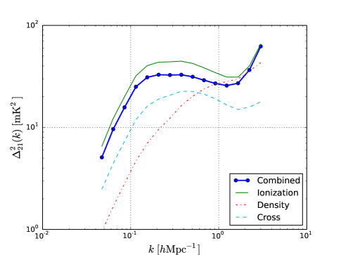
Figure 1: The spherically averaged dimensionless power spectrum of our fiducial model constructed using the quasi-linear approximation of Equation 1 (solid blue). The individual components are shown as thinner lines. The combined quasi-linear power spectrum is less than that of the ionization power spectrum because the correlation between the ionization and density fields, $P_{\delta_{\rho_{\rm{HI}}},\delta_{\rho_{\rm{H}}}}(k),$ (dashed cyan line) is negative; its absolute value is plotted here. This model was produced with simulations from 21cmFAST.

Note that while one of the goals of redshift space distortion measurements will be to measure their effects at a number of different redshifts, we use a single redshift model for illustrative purpose here.

2.2 The Foreground Footprint

To model the effects of foregrounds in $(k_{\perp},k_{\parallel}$) space, we use the approach of Pober et al. (2013b) and Pober et al. (2014), where modes which fall inside the “wedge” are deemed contaminated and considered as if they were not measured. We consider the wedge as extending to the horizon limit (Parsons et al., 2012b), but do not exclude any further modes outside the horizon. The mapping of the horizon limit for a given baseline (which is equivalent to the maximum delay between the two antennas measured in light-travel time) to cosmological $k_{\parallel}$ modes is given in Parsons et al. (2012b) and Pober et al. (2014):

$$k_{\parallel,\rm{hor}}=\left(\frac{1}{\nu}\frac{Y}{X}\right)k_{\perp},$$ (5)

where $\nu$ is observing frequency, and $X$ and $Y$ are cosmological scalars for converting observed bandwidths and solid angles to $h{\rm Mpc}^{-1}$, respectively, defined in Parsons et al. (2012a) and Furlanetto, Oh & Briggs (2006). The cosmological scalars $X$ and $Y$ are of particular importance here; they depend on the angular diameter distance and Hubble constant at the redshift of the measurement, and can change significantly between the EoR experiments and the intensity mapping experiments discussed in §3. At the redshift of our fiducial power spectrum $z=9.5$ the horizon limit gives a slope of $k_{\parallel,\rm{hor}}=3.73k_{\perp}$.

The steepness of this slope is evident in Figure 2, which reproduces the wedge obtained from PAPER observations in Pober et al. (2013b). Unlike Pober et al. (2013b), here we plot the $k_{\parallel}$ and $k_{\perp}$ axes on the same scale to highlight another important feature of EoR 21 cm experiments: a mismatch between $k_{\perp}$ and $k_{\parallel}$ scales. The $k_{\perp}$ axis extends to $k_{\perp}=0.12h{\rm Mpc}^{-1}$, which corresponds to the longest baseline in the PAPER array of $\sim 300$ m. The $k_{\parallel}$ axis, however, is truncated; PAPER has a frequency resolution of 48.8 kHz, corresponding to a maximum $k_{\parallel}$ of $10.4~{}h{\rm Mpc}^{-1}$. The white lines show contours of constant $|k|$; even ignoring the wedge, a full range of $\mu$ is measured for only very small values of $|k|$. If modes within the wedge are considered contaminated, this loss of modes serves to set a minimum $\mu$ below which modes cannot be measured. For EoR observations at $z=9.5$, this value is $\mu_{\rm min}=0.966$. This large value of $\mu_{\rm min}$ is quite discouraging for EoR experiments looking to measure the effects of redshift space distortions: only with foreground removal working well into the wedge can a reasonable range of $\mu$ be recovered.

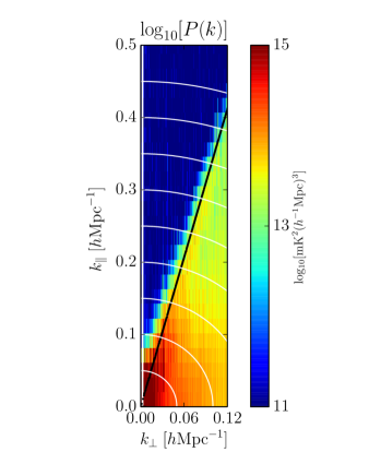
Figure 2: The foreground wedge as observed in PAPER data from Pober et al. (2013a). This plot differs from their Figure 3, in that the $k_{\parallel}$ and $k_{\perp}$ axes have been plotted in the same scale. The instrument measures much higher $k_{\parallel}$ modes than shown, but the $k_{\perp}$ cutoff is real and set by the longest baseline in the PAPER array. The black line shows the analytic horizon limit, and white lines show contours of constant $|k|$.

2.3 Sensitivity Calculations

Despite the discouragingly large value of $\mu_{\rm min}$ when modes inside the wedge are excluded, there is still a small hope for making a redshift space distortion measurement using only a foreground avoidance approach. As Equation 1 shows, the density power spectrum enters as $\mu^{4}$. Therefore, even though the measurable range of $\mu$ is extremely limited, it is at high values of $\mu$, where the signal is changing most rapidly. It is therefore conceivable that for even measuring only modes outside the wedge, an EoR experiment could pick out the component of the power spectrum with a $\mu^{4}$ dependence with reasonable significance.

In this section, we look at the potential for 21 cm experiments to detect redshift space distortion effects in our fiducial power spectrum. To do so, we use a version of the 21cmSense code (Pober et al., 2013b, 2014) which has been modified to retain 2D ($k_{\perp},k_{\parallel})$ information (as opposed to the standard package, which performs a spherical average to 1D). Under the foreground avoidance paradigm, all modes which fall inside the analytic horizon limit (Equation 5) are treated as foreground contaminted and excluded from the sensitivity calculation. This choice of exclusion region constitutes a middle ground between a more conservative choice where an additive term is included to model “supra-horizon” emission (c.f. Figure 2) and a more optimistic choice where the primary field-of-view of the telescope is used instead of the horizon (e.g. Beardsley et al. 2013; Pober et al. 2014). While this may be a somewhat pessimistic choice for next generation arrays with small fields of view, it may also prove to be the case that foreground emission in primary beam sidelobes still overwhelms the 21 cm signal in higher $k_{\parallel}$ modes.

To calculate the ability to recover redshift space distortion information, we fit a quartic polynomial in the form of Equation 1 to $P(k,\mu)$ for bins of constant $|k|$. The constant term therefore recovers the isotropic ionization power spectrum at $|k|$, the quadratic term the ionization-density cross power spectrum, and the quartic term the density power spectrum. Given the difficult nature of the measurement, we consider two proposed next-generation experiments: HERA (Pober et al., 2014) and the core of Phase 1 of the SKA-Low (following the design specifications of Dewdney et al. 2013). We summarize the properties of these arrays in Table 1. We consider observations spanning 1080 hours using the observing strategy described in Pober et al. (2014).

Instrument	Number of Elements	Element Size $(\rm{m}^{2})$	Collecting Area $(\rm{m}^{2})$	Configuration
HERA	547	154	84,238	Filled 200 m hexagon
SKA1-Low	866	962	833,190	Filled 270 m core with Gaussian distribution beyond

Table 1: 21 cm Epoch of Reionization Experiment Properties

Figure 3 plots the power spectrum as a function of $\mu$ in one annulus of $|k|=0.18~{}h{\rm Mpc}^{-1}$.

Instrument	Constant	Quadratic	Quartic	Spherically Avg.
HERA	0.07	0.03	0.02	108.1
SKA	0.33	0.16	0.09	95.6

Table 2: First three columns: Detection significance (i.e. “number of sigmas”) for each of the three $\mu$ moments of the 21 cm power spectrum. Right hand column: Detection significance of the spherically averaged power spectrum. Despite very high SNR spherically averaged power spectrum measurements, the $\mu$ dependence cannot be recovered with any significance.

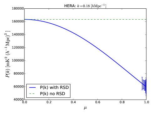
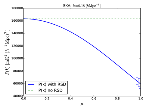
Figure 3: Potential measurements of HERA (left) and the SKA (right) of the 21 cm power spectrum as a function of $\mu$ for $|k|=0.18~{}h{\rm Mpc}^{-1}$. The blue line shows our fiducial 21 cm power spectrum including redshift space distortion effects, while the green dashed line contains only isotropic monopole term. No binning of the measurements has been performed; their spacing is set by the range of $k_{\perp}$ and $k_{\parallel}$ values probed by the instruments. Only one value of $|k|$ is plotted, but the results are generic for all $|k|$s: the foreground wedge limits measurements to $\mu>0.97$, severely hampering attempts to measure the redshift-space distortion signal (i.e. to detect any $\mu$-dependence in the power spectrum).

The green curve shows the value of the isotropic real-space power spectrum, while the blue curves shows the effect of redshift space distortions as decreasing the power at high $\mu$, the result of the negative sign of the density-ionization fluctuation cross power spectrum. At the $\mu$ values probed by EoR experiments, the decrease in power is of order a factor of 2. A more optimistic scenario might be to consider a redshift where the cross power spectrum is positive and redshift space distortions serve to boost the 21 cm signal. However, as will be shown below, the amplitude of the 21 cm power spectrum is not the limiting factor, as both arrays deliver very high significance measurements of the 1D spherically averaged power spectrum. The left hand plot shows the measurements and associated errors for HERA in this $|k|$ annulus, while the right shows those for the SKA.

Table 2 shows the “number of sigmas” at which each experiment constrains the three components (constant, quadratic, and quartic) of the redshift space power spectrum; while Figure 3 shows the measurements only in one $|k|$ bin, these numbers are for the cumulative measurement over all $|k|$s probed. These significances are calculated by including the calculated errors on each $k$ mode in the polynomial least-squares fit to the theoretical power spectrum, yielding total errors on the fit coefficients (which correspond to the three $\mu$ moments of the power spectrum). Also listed are the total significance values for measurements of the spherically averaged 1D power spectrum. While the spherically averaged power spectrum is measured with very high significance, it is clear that even the next generation of 21 cm EoR experiments will not make significant measurements of the redshift space distortion effects without a foreground subtraction technique that allows recovery of modes well inside the wedge. It should also be noted that without a full range of $\mu$ measurements, it will be difficult to separate the decrement of the power spectrum amplitude at high $\mu$ from the isotropic amplitude. This error will potentially bias the interpretation of initial spherically averaged power spectrum measurements, but attempting to quantify this effect is outside the scope of this present work.

3 Intensity Mapping Experiments

3.1 The Redshift Space Distortion Signal

The redshift space distortion signal is relatively simpler at the $z\sim 1-3$ measurements of intensity mapping experiments. At these redshifts, all the neutral hydrogen resides in self-shielded halos, which trace the matter power spectrum (Madau, Meiksin & Rees, 1997; Barkana & Loeb, 2007). Since the entirety of the 21 cm signal comes from only density fluctuations, there are no cross-correlation terms between different components. Furthermore, since 21 cm experiments are probing mainly large scales that have not gone non-linear by these redshifts, we use the Kaiser approximation to model redshift space distortions (Kaiser, 1987):

$$P(k,\mu)=(1+\beta\mu^{2})^{2}P(k),$$ (6)

where $\beta\equiv f/b$ (where $f$ is the logarithmic growth rate of structure $f\equiv d~{}\mathrm{ln}~{}D/d~{}\mathrm{ln}~{}a$ and $b$ is the bias of neutral hydrogen containing halos). A principal goal of redshift space distortions measurements at these redshifts is to constrain $\beta$, which has been measured to be $\approx\Omega_{m}^{0.6}$. (Fisher et al., 1994; Heavens & Taylor, 1995; Pápai & Szapudi, 2008; Percival & White, 2009). A detailed history of $\beta$ as a function of redshift can be used to trace the growth of structure over cosmic time and potentially even distinguish between dark energy and modified gravity as the cause of the observed late time acceleration in cosmic expansion (Percival & White, 2009; Song & Percival, 2009). In 21 cm measurements, there is also a degeneracy in the power spectrum amplitude between $b$ and $f_{\rm HI}$, the mass fraction of neutral hydrogen with respect to the cosmic baryon content, which can be broken by measuring the $\mu$ dependence of the power spectrum.

For our fiducial signal, we use a simulation of the matter power spectrum at $z=1.19$ from CAMB (Lewis, Challinor & Lasenby, 2000), multiplied by a scalar converting the matter power spectrum to 21 cm brightness temperature (Madau, Meiksin & Rees, 1997; Barkana & Loeb, 2007; Ansari et al., 2012; Pober et al., 2013b):

$$P(k)=\left[\tilde{T}_{21}(z)\right]^{2}b^{2}P_{\delta}(k),$$ (7)

$$\tilde{T}_{21}(z)\simeq 0.084{\rm mK}\frac{(1+z)^{2}h}{\sqrt{\Omega_{m}(1+z)^{3}+\Omega_{\Lambda}}}\frac{\Omega_{B}}{0.044}\frac{f_{\rm{HI}}(z)}{0.01},$$ (8)

where $\tilde{T}_{21}(z)$ is the mean 21cm brightness temperature at redshift $z$, $P_{\delta}(k)$ is the matter power spectrum, $\Omega_{\Lambda}$ is the cosmological constant, and $\Omega_{m}$ and $\Omega_{B}$ are the matter and baryon density in units of the critical density, respectively. Our fiducial value for $b$ is 1.5 (Chang et al., 2010). We plot a 1D spherical average of our fiducial power spectrum, including the redshift space effects of Equation 6, in Figure 4.

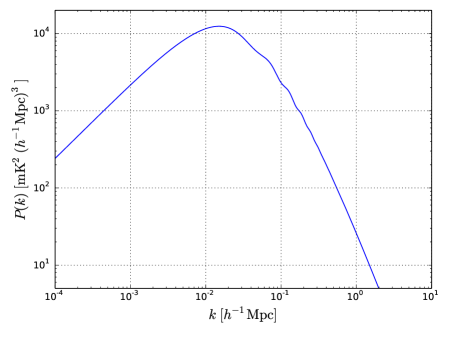
Figure 4: The spherically averaged 21 cm power spectrum at $z=1.19$ including redshift space distortion effects.

3.2 The Foreground Footprint

Evaluating Equation 5 for $z=1.19$ (650 MHz in the 21 cm line, near the center of band for a number of intensity mapping experiments) gives a horizon slope of $k_{\parallel,\mathrm{hor}}=0.77k_{\perp}$, a significantly shallower slope than at EoR redshifts. This fact mainly stems from the large evolution in the angular diameter distance and Hubble parameter between $z\sim 8$ and $z\sim 1$. The corresponding $\mu_{\rm min}$ for this horizon slope is 0.61; although a large range of $\mu$ is still excluded by the wedge, there remain enough high $\mu$ values that measuring redshift space distortions at $z\sim 1$ with a foreground avoidance strategy becomes a feasible proposition.

3.3 Sensitivity Calculations

Following the procedure described in §2.3, we calculate the sensitivities of three intensity mapping array concept designs to redshift space distortion signatures in our fiducial $z=1.19$ power spectrum: a 144-element BAOBAB-like array (Pober et al., 2013b), a 4096-element CHIME-like array (Shaw et al., 2014), and an SKA-Mid concept array meeting the design specifications of Dewdney et al. (2013) (although for simplicity the 64 MeerKAT dishes are assumed to be identical to the 190 SKA dishes).

Instrument	Number of Elements	Element Size $(\rm{m}^{2})$	Collecting Area $(\rm{m}^{2})$	Configuration
BAOBAB	144	6.25	900	Filled $12\times 12$ square
CHIME	4096	2.25	9,216	Filled $64\times 64$ square
SKA1-Mid	254	176.6	44,863	Random locations with power-law baseline distribution

Table 3: 21 cm Intensity Mapping Experiment Properties

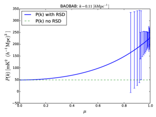
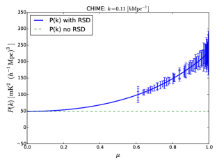
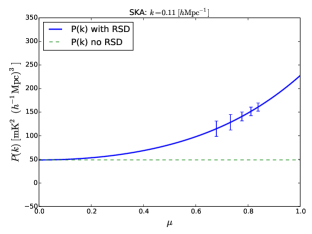
Figure 5: Potential measurements of BAOBAB (left), CHIME (center), and the SKA (right) of the 21 cm power spectrum as a function of $\mu$ for $|k|=0.11~{}h{\rm Mpc}^{-1}$ (BAOBAB and CHIME) and $|k|=0.27~{}h{\rm Mpc}^{-1}$ (SKA). The different $k$ mode and scale for the SKA results from the fact that it cannot probe the shorter $k=0.11~{}h{\rm Mpc}^{-1}$ mode at 600 MHz. The blue line shows our fiducial 21 cm power spectrum including redshift space distortion effects, while the green dashed line contains only isotropic monopole term. No binning of the measurements has been performed; their spacing is set by the range of $k_{\perp}$ and $k_{\parallel}$ values probed by the instruments. Only one value of $|k|$ is plotted, but the results are generic for all $|k|$s: low values of $\mu$ cannot be measured due to foregrounds, but enough measurements are possible to see the $\mu$ dependence introduced by redshift space distortions. Only CHIME has enough SNR to fit the functional form of the power spectrum and recover cosmological information.

Instrument	Constant	Quadratic	Quartic	Spherically Avg.	$\beta$ (frac. err.)
BAOBAB	0.4	0.3	0.26	23.1	1.99
CHIME	5.7	4.3	3.4	205.8	0.15
SKA	1.8	1.4	1.1	65.66	0.47

Table 4: Detection significance (i.e. “number of sigmas”) for each of the three $\mu$ moments of the 21 cm power spectrum, followed by the total detection significance of the spherically averaged 21 cm power spectrum. The right-hand column shows the achievable fractional error on $\beta$. Only CHIME produces measurements that are of any cosmological significance.

The configuration details of these arrays are described in Table 3, and their achievable constraints on the redshift space distortion signal are presented in Table 4. For each array, we calculate the sensitivities for a 100 MHz band centered on 650 MHz $(z=1.19)$; most of these experiments have wider bandwidths (e.g. $400-800$ MHz for CHIME), and so will be able to deliver measurements over a range of redshifts simultaneously.

We see that the relatively smaller BAOBAB-like array cannot make a significant measurement of the redshift space distortion terms, while the CHIME-like instrument can reach moderate significances. The SKA design does poorly, despite its large collecting area; this is because the minimum measurable $k_{\perp}$ for the 15 m dish of the SKA is $0.07~{}h{\rm Mpc}^{-1}$. This scale is just beyond the peak of the power spectrum, and the vast majority of baselines are significantly longer. Put another way, the SKA Mid design is not tuned for measuring the large-scale structure of the neutral hydrogen power spectrum. Example measurements at $k=0.11\ h{\rm Mpc}^{-1}$ are shown for the BAOBAB-like, CHIME-like, and SKA arrays in Figure 5. As noted, the SKA has very few measurements at this small value of $|k|$. On the other hand, the BAOBAB-like array does not have measurements reaching down to $\mu_{\rm min}$ because it does not have enough long baselines to measure $|k|=0.11\ h{\rm Mpc}^{-1}$ modes with a significant transverse component. At smaller values of $|k|$ than plotted, the full accessible range of $\mu$ is recovered.

In Table 4, we also present the achievable fractional error on $\beta$, calculated by taking ratios of different power spectrum moments to cancel out uncertainties in other parameters and then propagating theoretical uncertainties. Although more sophisticated analyses techniques now exist for redshift-space distortion measurements (e.g. Percival & White 2009), we present constraints using simple calculations as illustrative of the instrument sensitivities. Presumably, more advanced analyses could be used to improve these measurements. Under this framework, a CHIME-like experiment can yield 15% errors on $\beta$, comparable to the last generation of galaxy surveys (Percival et al., 2004; Ross et al., 2007), while neither the smaller BAOBAB-like instrument nor the SKA with its very long baselines can make a significant measurement. With significant constraints on $\beta$, an experiment can also break the degeneracy between $\beta$ and $f_{\rm HI}$ in setting the amplitude of the spherically averaged 21 cm power spectrum. Finally, it is worth repeating that these measurement errors come from a 100 MHz band, meaning that the redshift dependence of $\beta$ over the CHIME band should be measurable.

To explore the broader potential of 21 cm experiments, we consider a “no-foreground” case measurement with the CHIME-like array. While a completely foreground free measurement is impossible (the spectral modes inherent in the foreground spectrum cannot be separated from those modes in the 21 cm spectrum), this case serves to illustrate the limitations of our foreground avoidance technique. In this scenario, we obtain 2.5% errors in a measurement of $\beta$. While these errors could be further decreased by observing more fields of view, it is clear that percent-level errors on $\beta$ will be very difficult to achieve.

4 Discussion and Conclusions

In this paper, we have explored the effect of the redshift space anisotropy of foregrounds on measuring and recovering cosmological information from the redshift space anisotropy of the cosmological 21 cm signal. While a foreground avoidance approach has proven theoretically (Parsons et al., 2012b; Pober et al., 2014) promising and has yielded the best upper limit of the EoR signal to date (Parsons et al., 2014), this technique severely limits the amount of information that can be gleaned from redshift space distortions. For 21 cm experiments at EoR redshifts, the foreground wedge contaminates nearly all values of $\mu=k_{\parallel}/|k|$; at 150 MHz, for example, all modes with $\mu<0.97$ will be corrupted by foregrounds without applying some foreground removal/subtraction. While measuring the $\mu^{4}$ moment of the 21 cm power spectrum could potentially probe the matter power spectrum at high redshift, the effect of the foreground-imposed $\mu$ cut-off is to prevent any high-significance measurement even for planned large experiments like HERA and the SKA.

The situation is somewhat more promising for lower redshift “intensity mapping” experiments. While foregrounds still prevent recovery of low $\mu$ modes, the window for making 21 cm measurements is much larger. This difference is due to the large evolution in the Hubble parameter and angular diameter distance between redshifts $z~{}\sim~{}8$ and $z~{}\sim~{}1$. These cosmological parameters determine the mapping of angular and frequency values in data to $k_{\perp},k_{\parallel}$ coordinates, with the effect of making the wedge much smaller at lower redshifts. In our calculations at $z=1.19$ over half of $\mu$ modes still fall within the foreground wedge; however, since the redshift space distortion signals are (to first approximation) quadratic and quartic in $\mu$, larger values of $\mu$ are better for distinguishing the signal from the $\mu$-independent monopole. For a large 21 cm experiment optimized for intensity mapping like CHIME, foreground avoidance will still allow for the recovery of cosmological information from the redshift space signal. Smaller experiments like BAOBAB and less-optimized experiments like the SKA, however, still cannot recover the signal.

While this work has primarily considered a foreground avoidance technique, a “foreground-free” scenario was shown to increase intensity mapping constraints by as much as $\sim 7$. While a no foreground scenario is clearly implausible, further development of foreground removal algorithms should allow for additional sensitivity in redshift space distortion measurements with the 21 cm line. Even if the end result of foreground subtraction is only to push the wedge back from the horizon limit, this will have the effect of lowering the minimum measurable $\mu$ mode, and so further open the window on 21 cm redshift space distortion measurements.

References

- Ansari et al. (2012) Ansari R., Campagne J.-E., Colom P., Magneville C., Martin J.-M., Moniez M., Rich J., Yèche C., 2012, Comptes Rendus Physique, 13, 46
- Barkana & Loeb (2005) Barkana R., Loeb A., 2005, ApJL, 624, L65
- Barkana & Loeb (2007) Barkana R., Loeb A., 2007, Reports on Progress in Physics, 70, 627
- Beardsley et al. (2013) Beardsley A. P. et al., 2013, MNRAS, 429, L5
- Bharadwaj & Srikant (2004) Bharadwaj S., Srikant P. S., 2004, Journal of Astrophysics and Astronomy, 25, 67
- Bowman et al. (2013) Bowman J. D. et al., 2013, Publications of the Astronomical Society of Australia, 30, 31
- Chang et al. (2010) Chang T.-C., Pen U.-L., Bandura K., Peterson J. B., 2010, Nature, 466, 463
- Datta, Bowman & Carilli (2010) Datta A., Bowman J. D., Carilli C. L., 2010, ApJ, 724, 526
- Dewdney et al. (2013) Dewdney P. E., Turner W., Millenaar R., McCool R., Lazio J., Cornwell T. J., 2013, SKA1 System Baseline Design. Tech. rep., SKA Program Development Office, Document Number: SKA-TEL-SKO-DD-001
- Fisher et al. (1994) Fisher K. B., Davis M., Strauss M. A., Yahil A., Huchra J. P., 1994, MNRAS, 267, 927
- Furlanetto, Oh & Briggs (2006) Furlanetto S. R., Oh S. P., Briggs F. H., 2006, Phys. Rep., 433, 181
- Heavens & Taylor (1995) Heavens A. F., Taylor A. N., 1995, MNRAS, 275, 483
- Jackson (1972) Jackson J. C., 1972, MNRAS, 156, 1P
- Jensen et al. (2013) Jensen H. et al., 2013, MNRAS, 435, 460
- Kaiser (1987) Kaiser N., 1987, MNRAS, 227, 1
- Lewis, Challinor & Lasenby (2000) Lewis A., Challinor A., Lasenby A., 2000, ApJ, 538, 473
- Lidz et al. (2007) Lidz A., Zahn O., McQuinn M., Zaldarriaga M., Dutta S., Hernquist L., 2007, ApJ, 659, 865
- Lonsdale et al. (2009) Lonsdale C. J. et al., 2009, IEEE Proceedings, 97, 1497
- Madau, Meiksin & Rees (1997) Madau P., Meiksin A., Rees M. J., 1997, ApJ, 475, 429
- Majumdar, Bharadwaj & Choudhury (2013) Majumdar S., Bharadwaj S., Choudhury T. R., 2013, MNRAS, 434, 1978
- Mao et al. (2012) Mao Y., Shapiro P. R., Mellema G., Iliev I. T., Koda J., Ahn K., 2012, MNRAS, 422, 926
- Mao et al. (2008) Mao Y., Tegmark M., McQuinn M., Zaldarriaga M., Zahn O., 2008, Phys. Rev. D, 78, 023529
- McQuinn et al. (2006) McQuinn M., Zahn O., Zaldarriaga M., Hernquist L., Furlanetto S. R., 2006, ApJ, 653, 815
- Mellema et al. (2013) Mellema G. et al., 2013, Experimental Astronomy, 36, 235
- Mesinger & Furlanetto (2007) Mesinger A., Furlanetto S., 2007, ApJ, 669, 663
- Mesinger, Furlanetto & Cen (2011) Mesinger A., Furlanetto S., Cen R., 2011, MNRAS, 411, 955
- Morales et al. (2012) Morales M. F., Hazelton B., Sullivan I., Beardsley A., 2012, ApJ, 752, 137
- Morales & Wyithe (2010) Morales M. F., Wyithe J. S. B., 2010, ARA&A, 48, 127
- Pápai & Szapudi (2008) Pápai P., Szapudi I., 2008, MNRAS, 389, 292
- Parsons et al. (2012a) Parsons A., Pober J., McQuinn M., Jacobs D., Aguirre J., 2012a, ApJ, 753, 81
- Parsons et al. (2010) Parsons A. R. et al., 2010, AJ, 139, 1468
- Parsons et al. (2014) Parsons A. R. et al., 2014, ApJ, 788, 106
- Parsons et al. (2012b) Parsons A. R., Pober J. C., Aguirre J. E., Carilli C. L., Jacobs D. C., Moore D. F., 2012b, ApJ, 756, 165
- Percival et al. (2004) Percival W. J. et al., 2004, MNRAS, 353, 1201
- Percival & White (2009) Percival W. J., White M., 2009, MNRAS, 393, 297
- Pober et al. (2014) Pober J. C. et al., 2014, ApJ, 782, 66
- Pober et al. (2013a) Pober J. C. et al., 2013a, ApJL, 768, L36
- Pober et al. (2013b) Pober J. C. et al., 2013b, AJ, 145, 65
- Pritchard & Loeb (2012) Pritchard J. R., Loeb A., 2012, Reports on Progress in Physics, 75, 086901
- Ross et al. (2007) Ross N. P. et al., 2007, MNRAS, 381, 573
- Sargent & Turner (1977) Sargent W. L. W., Turner E. L., 1977, ApJL, 212, L3
- Shaw et al. (2014) Shaw J. R., Sigurdson K., Pen U.-L., Stebbins A., Sitwell M., 2014, ApJ, 781, 57
- Song & Percival (2009) Song Y.-S., Percival W. J., 2009, Journal of Cosmology and Astroparticle Physics, 10, 4
- Thyagarajan et al. (2013) Thyagarajan N. et al., 2013, ApJ, 776, 6
- Tingay et al. (2013) Tingay S. J. et al., 2013, Publications of the Astronomical Society of Australia, 30, 7
- Trott, Wayth & Tingay (2012) Trott C. M., Wayth R. B., Tingay S. J., 2012, ApJ, 757, 101
- van Haarlem et al. (2013) van Haarlem M. P. et al., 2013, A&A, 556, A2
- Vedantham, Udaya Shankar & Subrahmanyan (2012) Vedantham H., Udaya Shankar N., Subrahmanyan R., 2012, ApJ, 745, 176
- Xu, Wang & Chen (2014) Xu Y., Wang X., Chen X., 2014, ArXiv e-prints, arXiv:1410.7794
- Yatawatta et al. (2013) Yatawatta S. et al., 2013, A&A, 550, A136
- Zaroubi (2013) Zaroubi S., 2013, in Astrophysics and Space Science Library, Vol. 396, Astrophysics and Space Science Library, Wiklind T., Mobasher B., Bromm V., eds., p. 45