Coexistence of phases in asymmetric nuclear matter under strong magnetic fields

Abstract

The equation of state of nuclear matter is strongly affected by the presence of a magnetic field. Here we study the equilibrium configuration of asymmetric nuclear matter for a wide range of densities, isospin composition, temperatures and magnetic fields. Special attention is paid to the low density and low temperature domain, where a thermodynamical instability exists. Neglecting fluctuations of the Coulomb force, a coexistence of phases is found under such conditions, even for extreme magnetic intensities. We describe the nuclear interaction by using the non–relativistic Skyrme potential model within a Hartree–Fock approach. We found that the coexistence of phases modifies the equilibrium configuration, masking most of the manifestations of the spin polarized matter. However, the compressibility and the magnetic susceptibility show clear signals of this fact. Thermal effects are significative for both quantities, mainly out of the coexistence region.

I Introduction

The dense nuclear matter under magnetic fields has been intensively studied (see LAI and references therein), particularly in relation to astrophysical issues. Investigations of the neutron star structure LATTIMER as well as the cooling of magnetized stars SHIBANOV ; YAKOVLEV ; BEZCHASTNOV need the equation of state for magnetized matter as an important input. The presence of very intense magnetic fields in compact stellar objects has been proposed, based on the observational evidence of periodic or irregular radiation from localized sources. According to the energy released and the periodicity of the episodes, these objects have been classified as pulsars, soft gamma ray repeaters and anomalous X-ray pulsars. They have been associated with different stages of the evolution of neutron stars. On the star surface the magnetic field could reach values $10^{14}-10^{15}$ G, as in the case of magnetars and it is expected a growth of several orders of magnitude in its dense interior.

Recent investigations KHARZEEV ; MO ; SKOKOV have pointed out that matter created in heavy ion collisions could be subject to very strong magnetic fields. As a consequence the particle production would exhibit a distinguishable anisotropy. A preferential emission of charged particles along the direction of the magnetic field is predicted in KHARZEEV for noncentral heavy ion collisions, due to magnetic intensities $e\,B\sim 10^{2}$ MeV. Improved calculations taking care of the mass distribution of the colliding ions MO , does not modify essentially the magnitude of the produced fields. Furthermore, the numerical simulations performed by SKOKOV predict larger values $e\,B\sim m_{\pi}^{2}\sim 2\times 10^{4}$ MeV².

The effects of magnetic fields on a dense nuclear environment have been described using different models CHAKRABARTY ; BRODERICK ; YUE2 ; SINHA ; RABHI ; RYU ; RYU2 ; ANG ; DONG ; DIENER ; DONG2 ; PGARCIA ; ISAYEV ; UNLP ; UNLP2 ; BORDBAR ; BIGDELI2 . For instance, covariant field theoretical models have been used to study the role of the magnetic field on hyperonic matter YUE2 ; SINHA , instabilities at subsaturation densities RABHI ; RYU , magnetization of stellar matter DONG , saturation properties of symmetric matter DIENER and the symmetry energy DONG2 . Non-relativistic models have also been used, in the effective interactions of PGARCIA ; ISAYEV ; UNLP or the microscopic models used in the variational calculations of BORDBAR ; BIGDELI2 . A comparison of neutron matter results, using different models was presented in UNLP2 .

It is a well known fact that the nuclear environment experiences thermodynamical instabilities at subnuclear densities and low temperatures. Evidence of this phenomenon can be found in the isospin distillation effect for heavy ion collisions DAS . These instabilities give rise to a coexistence of phases if the surface tension is low enough. A more complex scenario is obtained when an external magnetic field is added, since there is a competition among two opposite trends. On one hand the magnetic force induces a globally ordered state with aligned spins. On the other hand the nuclear interaction favors the coexistence of phases where two states of different densities and spin polarizations are combined in order to lower the free energy.

In the present work we explore the possibility of a coexistence of phases for nuclear matter under strong magnetic fields, taking as variables the nuclear density, the isospin composition of matter, and the temperature $T<10$ MeV. The possible fields of applications, such as those mentioned before, show a complex scenario where the detailed physical mechanisms are not easy to understand because there is a superposition of effects which can combine to give very different manifestations. Therefore, we aim to present here some of the variables appearing in realistic situations, emphasizing the role of each of these factors, and to understand how they interact in a specific environment. Special attention is paid to the relevant quantities associated with them, as the spin polarization, the isothermal compressibility and the magnetic susceptibility. With this purpose in mind we have analyzed a wide range of isospin composition and we have also reached the extreme value $B=10^{19}$ G for the external magnetic field. This selection emphasizes the effects of these variables, which under certain conditions can appear weakened, or hidden by another factors.

The Skyrme model SKYRME ; DOUCHIN ; BENDER1 ; BENDER2 is appropriate to describe the nuclear interaction under the conditions of interest. This is a non-relativistic effective model where the in–medium nuclear force is simulated by a density dependent potential. It was successfully used to describe atomic nuclei as well as nuclear matter properties.

This article is organized as follows. We review the Skyrme model for nuclear matter under an external magnetic field in the next section, a brief resume of the Gibbs construction for the coexistence of phases is presented in Section III, the results are shown and discussed in Section IV. A final summary and the main conclusions are given in Section V.

II Spin polarized nuclear matter in the Skyrme model

The Skyrme model is an effective formulation of the nuclear interaction which has been employed profusely in the literature BENDER1 . It consists of a basic Hamiltonian with contact nucleon-nucleon potentials including density dependent coefficients,

$$v_{Sky}(r_{1},r_{2}) = t_{0}(1+x_{0}\,P_{\sigma})\delta(r_{1}-r_{2})+\frac{1}{2}t_{1}(1+x_{1}\,P_{\sigma})\left[\stackrel{{\scriptstyle\leftarrow}}{{q}}^{2}\delta(r_{1}-r_{2})+\stackrel{{\scriptstyle\rightarrow}}{{q}}^{2}\delta(r_{1}-r_{2})\right]$$

$$+ t_{2}(1+x_{2}\,P_{\sigma})\stackrel{{\scriptstyle\leftarrow}}{{q}}\cdot\delta(r_{1}-r_{2})\stackrel{{\scriptstyle\rightarrow}}{{q}}+\frac{1}{6}t_{3}(1+x_{3}\,P_{\sigma})\delta(r_{1}-r_{2})n^{\sigma}((r_{1}+r_{2})/2)$$

$$+ iW_{0}(\sigma_{1}+\sigma_{2})\cdot\stackrel{{\scriptstyle\leftarrow}}{{q}}\times\delta(r_{1}-r_{2})\stackrel{{\scriptstyle\rightarrow}}{{q}}$$

where $\sigma_{k}$ represent the Pauli matrices for spin, $P_{\sigma}=(1+\sigma_{1}\cdot\sigma_{2})/2$ is the spin exchange operator, $q=-i(\nabla_{1}-\nabla_{2})/2$ is the relative momentum operator and $n$ is the total baryonic density.
Note that throughout this article we use units such that $c=1$, $\hbar=1$.
The interaction–parameters are fixed to cover a variety of applications such as exotic nuclei or stellar matter. Using the Hartree-Fock approximation, one can find an energy density functional, which is a convenient way to study thermodynamical properties of the system.

We are particularly interested in the contributions coming from terms containing time reversal-odd densities and currents, since they are active when spin states are not symmetrically occupied. A derivation of these terms can be found in BENDER2 . We assume the magnetic field has not dynamics, that is, it behaves as an external field. There is a direct coupling between nucleons and the magnetic field, due to their intrinsic magnetic moments. This implies an additional term $-\mu_{N}\chi_{a}B$ to the single particle spectra of the standard Skyrme model, where $\mu_{N}$ is the Bohr magneton and the Lande factors $\chi_{a}$ take account of the anomalous magnetic moments. They take the values $\chi_{1}=2.793$ and $\chi_{2}=-1.913$ for protons and neutrons, respectively.
Furthermore, the magnetic field induce a quantization of the energy spectra of charged particles LANDAU . In the case of a uniform field, the corresponding Schrödinger equation exhibits quantized eigenvalues, associated with the motion in directions orthogonal to the applied field. They are oscillator-like levels, depending on a discrete quantum number in the form $(j+1/2)\,\omega$, with $\omega=eB/m$ the cyclotron frequency of the particle. We can summarize the effects of a uniform magnetic field over the spectra of nucleons by

$$\varepsilon_{1sj}(p_{z}) = \frac{p_{z}^{2}}{2m^{*}_{1s}}+\frac{1}{8}v_{1s}+\mu_{N}B(2j+1-s\chi_{1}),$$ (1)

$$\varepsilon_{2s}(p) = \frac{p^{2}}{2m^{*}_{2s}}+\frac{1}{8}v_{2s}-\mu_{N}Bs\chi_{2}.$$ (2)

The first two terms in the r.h.s of these equations, are the common results for the Skyrme model, which now have an implicit dependence on the field $B$. The spin index $s=1$ ($s=-1$) denotes a spin–up (spin–down) projection, the effective nucleon mass $m^{*}_{as}$ is defined by

$$\frac{1}{m^{*}_{as}}=\frac{1}{m}+\frac{1}{4}\,n\,(b_{0}-b_{2}wI_{a})+\frac{1}{4}\,s\sum_{b}(b_{1}+I_{a}I_{b}b_{3})\;W_{b}$$ (3)

with $m$ the degenerate nucleon mass in vacuum, $w=(n_{2}-n_{1})/n$ is the isospin asymmetry fraction, with $n_{1},\,n_{2}$ standing for the particle number density of protons and neutrons respectively. Note that $n=n_{1}+n_{2}$. Since the spin states are not symmetrically occupied, one can define for each isotopic component the number density of particles with a given spin polarization $n_{a\,s}$. The spin asymmetry density $W_{a}$ gives a measure of the spin polarization $W_{a}=\sum_{s}s\,n_{a\,s}$, clearly $n_{a}=\sum_{s}n_{a\,s}$. We have defined $I_{a}=1,\;(-1)$ for protons (neutrons).
In Eqs. (1) and (2) we have used the single particle Skyrme potential energy

$$v_{as} = (a_{0}-a_{2}wI_{a})\,n+\sum_{s^{\prime}c}(b_{0}+I_{a}I_{c}b_{2})K_{cs^{\prime}}+s\sum_{c}(a_{1}+a_{3}I_{a}I_{c})W_{c}+$$ (4)

$$+s\sum_{s^{\prime}c}s^{\prime}(b_{1}+b_{3}I_{a}I_{c})K_{cs^{\prime}}.$$

The expressions for the kinetic energy density $K_{as}$ will be presented below. The Eqs. (1)–(4) have been written in terms of a set of density dependent coefficients $a_{0}-a_{3}$ and $b_{0}-b_{3}$, which are related to the standard parameters of the Skyrme model by,

$$a_{0} = 6t_{0}+t_{3}n^{\sigma},$$

$$b_{0} = [3t_{1}+t_{2}(5+4x_{2})]/2$$

$$a_{1} = -2t_{0}(1-2x_{0})-t_{3}(1-2x_{3})n^{\sigma}/3$$

$$b_{1} = [t_{2}(1+2x_{2})-t_{1}(1-2x_{1})]/2$$

$$a_{2} = -2t_{0}(1+2x_{0})-t_{3}(1+2x_{3})n^{\sigma}/3$$

$$b_{2} = [t_{2}(1+2x_{2})-t_{1}(1+2x_{1})]/2$$

$$a_{3} = -2t_{0}-t_{3}n^{\sigma}/3$$

$$b_{3} = (t_{2}-t_{1})/2$$

We assume baryonic and isospin number conservation, therefore independent chemical potential $\mu_{a}$ can be assigned to protons and neutrons. The corresponding distribution functions $f_{as}(T,p)=\left[1+\exp(\varepsilon_{as}(p)-\mu_{a})/T\right]^{-1}$ are the Fermi occupation number for a particle at temperature $T$, with momentum $p$ and isospin and spin projections $a$ and $s$, respectively.

Now we show explicit expressions for the density of particles with a given spin polarization, the kinetic energy and the isospin asymmetry densities, separately for protons and neutrons

$$n_{1s} = \frac{eB}{(2\pi)^{2}}\sum_{j}\int_{-\infty}^{\infty}dp_{z}\;f_{1sj}(T,p_{z})$$ (5)

$$W_{1} = \frac{eB}{(2\pi)^{2}}\sum_{s,j}s\int_{-\infty}^{\infty}dp_{z}\;f_{1sj}(T,p_{z})$$ (6)

$$K_{1s} = \frac{eB}{(2\pi)^{2}}\sum_{j}\int_{-\infty}^{\infty}dp_{z}\;p_{z}^{2}f_{1sj}(T,p_{z})$$ (7)

$$n_{2s} = \frac{1}{(2\pi)^{3}}\int d^{3}p\;f_{2s}(T,p)$$ (8)

$$W_{2} = \sum_{s}\frac{s}{(2\pi)^{3}}\int d^{3}p\;f_{2s}(T,p)$$ (9)

$$K_{2s} = \frac{1}{(2\pi)^{3}}\int d^{3}p\;p^{2}f_{2s}(T,p)$$ (10)

For the proton related quantities, we have taken into account that, assuming $B$ along the z-axis, each eigenstate spreads over a bounded region of area $2\pi eB$ in the $p_{x}-p_{y}$ plane. The component $p_{z}$ is not bounded and varies continuously. Therefore, the contribution of a charged particle to macroscopic quantities per unit volume has been evaluated by means of the replacement $\int d^{3}p/(2\pi)^{3}\rightarrow eB\int dp_{z}/(2\pi)^{2}$.

The energy density can be split into two terms,

$$\mathcal{E}=\mathcal{E}_{Skm}+\mu_{N}B\left(2L+n_{1}-\chi_{1}W_{1}-\chi_{2}W_{2}\right),$$ (11)

one of them depends on $B$. The remaining one is similar to the common contribution of the Skyrme model ${\mathcal{E}}_{Skm}$ in a Hartree-Fock approach, but now it depends implicitly on the magnetic intensity

$${\mathcal{E}}_{Skm}=\sum_{a,s}\,\frac{K_{as}}{2m^{*}_{as}}+\frac{1}{16}\left[a_{1}\left(\sum_{a}W_{a}\right)^{2}+a_{3}\left(\sum_{a}I_{a}W_{a}\right)^{2}+(a_{0}+a_{2}w^{2})\;n^{2}\right].$$ (12)

In Eq. (11) we used,

$$L=\frac{eB}{(2\pi)^{2}}\sum_{s,j}j\int_{-\infty}^{\infty}dp_{z}\;f_{1sj}(T,p_{z}).$$ (13)

For completeness we also show the expression for the entropy density ${\cal S}$ in the quasi-particle approach,

$${\cal S} = {\cal S}_{1}+{\cal S}_{2},$$

$${\cal S}_{1} = -\frac{eB}{(2\pi)^{2}}\sum_{s,j}\int_{-\infty}^{\infty}dp_{z}\;\left[f_{1sj}\ln\left(f_{1sj}\right)+\left(1-f_{1sj}\right)\,\ln\left(1-f_{1sj}\right)\right],$$

$${\cal S}_{2} = -\sum_{s}\frac{1}{(2\pi)^{3}}\int d^{3}p\;\left[f_{2s}\ln\left(f_{2s}\right)+\left(1-f_{2s}\right)\,\ln\left(1-f_{2s}\right)\right]$$

The entropy is needed to build up the free energy $\mathcal{F}=\mathcal{E}-T\mathcal{S}$ and the pressure $P=\sum_{a}\mu_{a}n_{a}-\mathcal{F}$. The magnetization of the system $\mathcal{M}$ is evaluated in terms of the grand canonical potential $\Omega(\mu_{k},T,V)$ according to PATHRIA ,

$$\mathcal{M}=\frac{1}{V}\left(\frac{\partial\Omega}{\partial B}\right)_{\mu,T,V}.$$ (14)

For the system considered, we have $\Omega=-P\,V$. As expected, it can be decomposed into proton and neutron contributions $\mathcal{M}=\mathcal{M}_{1}+\mathcal{M}_{2}$. Finally, the standard relations are used for the isothermal compressibility $K$ and magnetic susceptibility $\chi$,

$$K = -\frac{1}{V}\left(\frac{\partial V}{\partial P}\right)_{N_{1},N_{2},T,B}$$

$$\chi_{a} = \left(\frac{\partial\mathcal{M}_{a}}{\partial B}\right)_{N,T,V}$$

Note that in our scheme we were able to develop analytical expressions for the isothermal compressibility and magnetic susceptibility. This gives us some confidence in the evaluation of these magnitudes, as for instance, the susceptibility for low temperatures has fast variations with the density.

In our approach both proton and neutron numbers are conserved separately, therefore the states of polarization of each component are also independent. The global polarization is determined by the condition of minimum free energy $F$. This criterium differs from that in UNLP , where the Legendre transformed potential $\mathcal{F-M}B$ was used.

The equilibrium state has a variable spin configuration, depending on $n,\,w,\,T$ and $B$. As will be shown, in the low temperature and low density domain the coexistence of phases imposes a state with a lower degree of polarization than the case which does not consider the phase transition.

III Coexistence of phases in nuclear matter

The nuclear interaction gives rise to instabilities in a dense infinite medium at low temperatures. If the Coulomb interaction is taken into account and its fluctuations are included, a nucleation process can be found.
Under the hypothesis assumed in the present work, the system evolves through a succession of equilibrium states, where it decomposes spontaneously into two phases of different density and isospin composition. This phenomenon has been classified as a non–congruent phase transition SCHRAMM since there are two conserved charges, i.e. proton and neutron numbers. Its importance in the study of the in–medium nuclear interaction has been emphasized in recent investigations WEISE .

These two coexisting phases, distinguished in the following by superindices $a$ and $b$, have different numbers of proton and neutrons. However they are subject to the thermodynamical equilibrium conditions,

$$P(N_{1}^{a},N_{2}^{a},T,V^{a},B) = P(N_{1}^{b},N_{2}^{b},T,V^{b},B),$$ (15)

$$\mu_{1}(N_{1}^{a},N_{2}^{a},T,V^{a},B) = \mu_{1}(N_{1}^{b},N_{2}^{b},T,V^{b},B),$$ (16)

$$\mu_{2}(N_{1}^{a},N_{2}^{a},T,V^{a},B) = \mu_{2}(N_{1}^{b},N_{2}^{b},T,V^{b},B),$$ (17)

Furthermore, each phase contributes to every intensive additive physical quantity, such as the densities of energy, entropy, etc. Thus, the free energy per unit volume and the density number of nucleons for the whole system can be written as

$$\mathcal{F}(N_{1},N_{2},T,V,B) = (1-\lambda)\,\mathcal{F}(N_{1}^{a},N_{2}^{a},T,V^{a},B)+\lambda\,\mathcal{F}(N_{1}^{b},N_{2}^{b},T,V^{b},B),$$

$$n_{k} = (1-\lambda)\,n_{k}^{a}+\lambda\,n_{k}^{b},\;\;k=1,2$$

where the coefficient $\lambda$ can be interpreted as the fraction of the partial volume occupied by the state $b$, hence it is bounded by $0\leq\lambda\leq 1$.

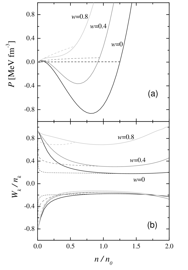
Figure 1: Details of the Gibbs construction for $B=10^{18}$ G at $T=5$ MeV and several isospin asymmetries. Panel (a) shows the pressure as a function of the density and panel (b) the spin asymmetry fraction as a function of the density. In the later case, the upper family of curves corresponds to the proton. Dashed lines correspond to the Gibbs construction.

In Fig. 1 it is shown how this procedure, commonly known as the Gibbs construction, works for the pressure and the spin asymmetry quotient of each component $W_{k}/n_{k}$. The general features of this figure will be discussed in the next section.

Following the standard thermodynamical definitions, the magnetization per unit volume, the magnetic susceptibility and the isothermal compressibility within the coexistence region can be evaluated as

$$\mathcal{M} = (1-\lambda)\,\mathcal{M}^{a}+\lambda\,\mathcal{M}^{b},$$ (18)

$$\chi_{k} = (1-\lambda)\,\chi_{k}^{a}+\lambda\,\chi_{k}^{b},\;\;k=1,2$$ (19)

$$K = \frac{(w^{a}-w^{b})\left[\lambda K^{b}+(1-\lambda)K^{a}\right]\,n^{a}\,n^{b}}{n\,\left[w\,(n^{b}-n^{a})+w^{a}n^{a}-w^{b}n^{b}\right]},$$ (20)

where $n^{a,\,b},\,w^{a,\,b}$ are the total density of particles and the isospin asymmetry fraction in each phase. The partial contributions to the magnetization $\mathcal{M}^{a,\,b}$, the susceptibility $\chi_{k}^{a,\,b}$ and the compressibility $K^{a,\,b}$ are evaluated in the same way as for a pure single phase.

IV Results and discussion

For the Skyrme model the SLy4 parametrization is used, for which $t_{0}=-2488.91$ MeV fm³, $t_{1}=486.82$ MeV fm⁵, $t_{2}=-546.39$ MeV fm⁵, $t_{3}=13777$ MeV fm^7/2, $x_{0}=0.834,\;x_{1}=-0.344,\;x_{2}=-1,\;x_{3}=1.354,\;\sigma=1/6$ DOUCHIN . The saturation density, binding energy, incompressibility and symmetry energy are $n_{0}=0.159$ fm^-3, $E_{B}=-15.97$ MeV, $K_{0}=229.9$ MeV and $E_{S}=32$ MeV, respectively. Another significative quantity is the in-medium nucleon mass at the saturation density, for which $m^{\ast}/m=0.694$ is obtained.

In first place we discuss the effects of the Gibbs construction on the pressure and the spin asymmetry coefficient $W/n$. These results are shown in Fig. 1, for $B=10^{18}$ G and $T=5$ MeV, which is representative for most of the cases studied in this work. The Gibbs construction is shown in dashed lines and replaces, within the coexistence region (CR), the plain results of the model described in Section II. In panel (a) it is shown that the CR includes the instability region where the pressure decreases with density. The Gibbs construction instead, produces a rather linear increasing pressure. The density domain of the CR is reduced and eventually vanishes, by increasing the isospin asymmetry $w$, as well as the temperature (not shown in this figure). For certain values of temperature and magnetic intensity, as for example $B=10^{18}$ G, $T=10$ MeV, the CR disappears for asymmetries above a typical value $w_{0}<1$. In these cases and for $w\simeq w_{0}$, a retrograde phase transition takes place. This means that the transition starts and ends at states of similar density and isospin composition, but in between an admixture with states of very different conditions is developed. We illustrate this phenomenon by including afterwards the case $B=10^{18}$ G, $T=10$ MeV, $w=0.8$.

In the panel (b) of the same figure, we show the spin asymmetry. It can be seen that protons and neutrons are highly polarized at very low densities and they depolarize progressively as the density grows. The coexistence of phases induces an equilibrium state with a significantly reduced degree of polarization, due to the admixture with a higher density and weaker polarization state. For higher magnetic intensities, such as $B=10^{19}$ G, the same mechanism causes the frustration of the total neutron magnetization, but it is not able to destroy the magnetic saturation of the proton, as will be discussed subsequently.

The behavior of the pressure as a function of the density for several temperatures and isospin asymmetries is shown in Fig. 2 for $B=10^{18}$ G and Fig. 3 for $B=10^{19}$ G. The points where a sudden change of slope occurs, correspond to an endpoint of the CR. They do not appear for some particular cases at $T=10$ MeV, because the coexistence does not exist for $B=10^{19}$ G and $w=0.8$ (Fig. 3b), whereas a retrograde transition goes on for $w=0.8$, $B=10^{18}$ G (Fig. 2b), as explained above. For a given magnetic intensity, thermal effects are more important for lower densities. Furthermore, an increase of the magnetic intensity at constant temperature induces an evident increment of the pressure for $n/n_{0}\lesssim 1$, but the opposite trend is observed for $n/n_{0}>1$. It must be pointed out that the Gibbs construction eliminates all the instabilities for the range of densities and temperatures studied here. In particular there are no regions where the pressure decreases with the density.

The density dependence of the spin asymmetry fraction is shown in Fig. 4 for $T=5$, several values of $w$, $B=10^{18}$ G (Fig. 4a) and $B=10^{19}$ G (Fig. 4b). Thermal variations are of no relevance for this quantity. For the lower field intensity, the proton relative polarization is enhanced as $w$ decreases, whereas for the neutrons there is only a weak dependence on the isospin composition. For $B=10^{19}$ G, the proton component is completely polarized for all the range of $n$ and $w$. The effect of the medium polarization is emphasized in this case, as can be seen in the dependence on $w$ of the neutron spin asymmetry for $n/n_{0}>0.75$. For a fixed total density $n$, the neutron component is completely polarized for $w=0$ and is progressively depolarized as $w$ increases. This is a consequence of the dynamical coupling of protons and neutrons (see Eqs. (1)-(4)). It must be pointed out that both components, but specially protons in a high $w$ sample, tend to recover a high degree of polarization at densities $n/n_{0}>1.5$. This feature can be a manifestation of the abnormal spontaneous magnetization described by the Skyrme model at extreme densities.

Results for the free energy per volume $\cal{F}$ as a function of the density, are shown in Fig. 5 ($B=10^{18}$ G) and Fig. 6 ($B=10^{19}$ G). At relatively low densities the kinetic energy and the repulsion between nucleons are small, while the effect of the magnetic field becomes the dominant one. For medium and high densities the repulsive character of the nucleon-nucleon interaction and the kinetic energy dominate over the magnetic field and the system increases its energy. This is clearly depicted in Fig. 5, whereas for $B=10^{19}$ G in Fig. 6, only the $w=0.8$ case fits this description. For other values of $w$ one should go to higher densities to verify this behavior. From both figures we can see that the addition of protons makes the system to be more bound and so does the increase of the magnetic field. Thermal effects are weak, as opposite contributions tend to cancel each other: the kinetic term increases with $T$, while the entropy contribution does the opposite.

The magnetic susceptibility characterizes the response of the system to the external field and gives a measure of the energy required to produce a net spin alignment in the direction of the field. We have found that this quantity at moderate field intensities, is sensitive to thermal variations, hence we devote Figs. 7-9 to give a more detailed description of the density dependence of $\chi$. For all the cases shown, there is a low density regime where the system has an almost saturated magnetization (see Fig. 4), therefore the magnetic response is nearly zero. As it was previously discussed, in most cases the coexistence of phases frustrates the total magnetization and consequently enhances the magnetic response within the CR. This fact can be distinguished by an approximately linear increase, with a small slope, of the susceptibility as a function of the total density.
The magnetic susceptibility shows a complex dependence on the population of the Landau levels. Therefore, in order to clarify the discussion afterwards, it is worth to make some general considerations about this relationship. In first place it must be pointed out that the population of the Landau levels decreases with both $B$ and $w$, but it increases with both $n$ and $T$. However, the distribution function becomes smoother as the temperature grows, erasing eventually effects due to the progressive occupation of different Landau levels. In second place, when very high levels are occupied, further changes in the quantum number $j$ has only imperceptible consequences on the susceptibility. Finally, the proton component generally shows a diamagnetic behavior, but it turns to be paramagnetic when the statistical occupation is peaked at the lowest Landau level $j=0$.
Now we focus on the susceptibility for protons in the lower panel of Fig. 7, where the case of $B=10^{18}$ G and $T=1$ MeV, is illustrated. For increasing densities, the susceptibility changes from a linear response to an oscillatory behavior. The linear response turns out from the Gibbs construction, while the oscillatory behavior is a consequence of the population of the Landau levels. Note that in the evaluation of the partial contributions $\chi_{k}^{a,\,b}$ in Eq. (19), the Landau levels also play a role. However, the narrow range of variation of the densities $n^{a}$ and $n^{b}$ allows the linear behavior for the susceptibility. For $w=0$ and $w=0.4$ the system is diamagnetic, while for $w=0.8$ it is mainly paramagnetic due to the fact that only the lowest Landau levels are accessible. In the upper panel of the same figure, the neutron susceptibility is depicted. An important change in the scale is observed. The neutron susceptibility is always paramagnetic and also has a linear behavior for low densities which changes to oscillatory as the density grows. Even though neutrons do not have discrete levels, they are influenced by the dynamical coupling among protons and neutrons (see Eqs. (1)– (3)). For the case $w=0.8$ a sudden decrease at $n/n_{0}\approx 1.7$, is observed due to a change in the spin configuration of the system.

A small increase of the temperature, keeping fixed the magnetic intensity, destroys the oscillations at high densities. See Fig. 8 for $B=10^{18}$ G, $T=5$ MeV. The magnetic response of protons becomes almost linear for the full range of densities. Two ingredients contribute to these results: the distribution function becomes smoother as the temperature grows and the statistical occupation of the Landau levels increase, being this last effect the dominant one.

For the two figures just described, there is a noticeable difference of magnitude between the susceptibility of protons and neutrons. The proton component is significantly more reactive to changes of the magnetic intensity. The effects of changing the magnetic intensity by keeping fixed the temperature are exposed in Fig. 9, where we present the results for $B=10^{19}$ G, $T=5$ MeV. A dramatic change of scale is apparent for both components, but specially for protons. This fact is coherent with the saturation of proton spin alignment (see Fig. 4b), as a consequence the proton component experiences a change of regime from diamagnetic to paramagnetic. In contrast, neutrons which only have a paramagnetic channel, are completely blocked when the saturation of spin alignment is reached. Hence we have $\chi_{2}=0$, as for $w=0$. Note that for $B=10^{19}$ G, the statistical occupation of the Landau level is strongly dominated by $j=0$, which explains the paramagnetic behavior of the proton susceptibility.

In Figs. 10 and 11, the isothermal compressibility is presented as a function of the density for $B=10^{18}$ G and $B=10^{19}$ G, respectively. In both figures we show results for $T=1$, 5 and 10 MeV and isospin asymmetries $w=0$, 0.4 and 0.8. For all the cases shown, there is a clear difference between the CR and the domain of higher densities. In the last case, we found the typical behavior of an almost incompressible fluid with a slightly decreasing compressibility. Here the variation of temperature and isospin composition have weak effects, but they become appreciable for $B=10^{19}$ G. An exceptional behavior is found for $B=10^{19}$, $w=0$, $T=1$ MeV, where a local maximum can be seen around $n/n_{0}\cong 1.9$. It seems to be a feature of the model used and deserves a further investigation.
Within the CR, the compressibility decreases strongly for very low densities and becomes increasing for moderately higher values. As a consequence a local maximum of $K$ arises at the extreme point of the CR. This description applies strictly to the lowest temperature shown here, $T=1$ MeV. As $T$ is increased, the effect becomes less pronounced, but is still perceptible for $B=10^{19}$ G, whereas it is completely missed for $B=10^{18}$ G.

As the last matter of analysis we present in Fig. 12 the phase diagram for a fixed value $B=10^{19}$ G. Here the closed curves correspond to the isothermal contour of the CR, for both the $P-y$ (Fig. 12a) and $n-y$ (Fig. 12b) planes. The CR for a given temperature is enclosed by the corresponding curve. In the upper panel for each curve there is a maximum value for the pressure, at the left and below that pressure lies the lower density gaseous phase and, at the right the higher density liquid phase. Above that pressure a continuous passage from one phase to another occurs. As the temperature grows the area within the contour is reduced and eventually collapse to the critical point. Note that at very low pressures it is necessary to include states with a small proton excess in order to complete the phase diagram.

V Conclusions

In this work we have addressed the properties of asymmetric nuclear matter under the action of very strong magnetic fields , temperatures below $10$ MeV and densities up to twice the saturation density. For the nuclear interaction we have used the non–relativistic Skyrme potential model (SLy4 parametrization) within a Hartree–Fock approximation. We have paid special attention to the low–density and low–temperature domain, where the nuclear interaction gives rise to instabilities, commonly associated with a liquid-gas phase transition. If the Coulomb force is not included, the equilibrium state of the system separates spontaneously into coexisting phases. This phase transition was studied in detail in the past SCHRAMM ; WEISE and it has received renewed attention recently in connection with astrophysical investigations GIULANI and also in heavy–ion collisions, where the liquid–gas instabilities are related to the formation of fragments occurring in finite nuclear systems DAS .

Here we introduce an external magnetic field as a new parameter which modifies the properties of the coexisting phases. We propose and analyze the spin polarization, the magnetic susceptibility and the isothermal compressibility as physical quantities that reveal the changes in the global configuration as well as in the internal composition of the equilibrium state. A related investigation, but restricted to neutron matter, has been presented recently in UNLP2 . There, a comparison of the predictions of very different models was made, which give us some confidence about the common features and warn us about possible singularities of the model chosen.

To obtain the physical equation of state, we have implemented the so called Gibbs construction, which is the appropriate procedure when there are multiple conserved charges.

Referring to the spin polarization, it is higher for very low densities. Neutrons are in general less polarized than protons. At extreme intensities ($B=10^{19}$ G) the effect of the medium polarization is emphasized, due to the dynamical coupling of protons and neutrons (see Eqs. (1)-(4)) the relative magnetization of the neutrons is enhanced by increasing the proton fraction. The spin asymmetry depends weakly on the temperature, while it is strongly affected by the magnetic field. The spontaneous separation into independent phases reduces the degree of polarization for both protons and neutrons. This can be understood because for a given total density within the CR, one of such phases has a greater partial density and a lower polarization. This is the reason why neutrons do not reach the magnetic saturation at medium densities under the strongest intensity considered here.

The energy per volume shows that the addition of protons makes the system more bound. And so happens for increasing the magnetic field. At variance, the dependence with temperature is rather small.

The magnetic susceptibility is the most sensitive quantity, as it shows a strong dependence on the isospin asymmetry, the temperature and the magnetic intensity. For protons these dependencies manifest through the population of the Landau levels, which also reflects in the neutron susceptibility due to the dynamical coupling generated by the Skyrme model. The susceptibility in the CR is almost linear.

The isothermal compressibility at very low temperature offers a clear manifestation of the changes in the phase diagram. Out the CR the results corresponds to an almost incompressible fluid, decreasing slowly with density and showing a small dependence on $w,\,T$ and $B$. Within the CR, the compressibility changes from steeply decreasing at very low densities, to moderately increasing. In such a way a local maximum appears at the end of the CR. This behavior is attenuated by increasing the temperature.

An overview of the general phase diagram shows that the coexistence of phases exists for all the range of magnetic intensities of physical interest. The critical temperature lies above $T=10$ MeV. An increase of the magnetic field has multiple consequences, on one hand it produces an enhancement of the range of pressures involved, while does not modify the density domain. Furthermore the range of isospin asymmetries supported is reduced and for the higher $w$ the system evolves through a retrograde phase transition.

It is worthwhile to mention that most of this conclusions become evident because we used an extreme magnetic intensity. For weaker fields, effects such as the temperature-polarization antagonism or the synergistic combination of neutron excess and spin polarization, are still active but they manifest diffusely.

Figure 2: Pressure as a function of the density for $B=10^{18}$ G and several isospin fractions. Panel (a) corresponds to $T=5$ MeV and panel (b) to $T=10$ MeV.

Figure 3: The same as Fig. 2, but for $B=10^{19}$ G.

Figure 4: The spin asymmetry fraction of protons and neutrons as functions of the density at $T=5$ MeV and several isospin fractions. Panel (a) corresponds to $B=10^{18}$ G and panel (b) to $B=10^{19}$ G. In each panel the upper family of curves correspond to protons. The same convention line is used for both panels.

Figure 5: The free energy per volume as function of the density for $B=10^{18}$ G and several isospin fractions. Panel (a) corresponds to $T=1$ MeV , panel (b) to $T=5$ MeV and panel (c) to $T=10$ MeV. The same convention line is used for all the panels.

Figure 6: The same as Fig. 5, but for $B=10^{19}$ G.

Figure 7: The magnetic susceptibility (scaled with $\mu_{N}^{2}$) as function of the density for $B=10^{18}$ G at $T=1$ MeV and several isospin fractions. Panel (a) corresponds to neutrons and panel (b) to protons. The same convention line is used for both panels.

Figure 8: The same as Fig. 7, but for $T=5$ MeV.

Figure 9: The same as Fig. 7, but for $B=10^{19}$ G and $T=5$ MeV.

Figure 10: The isothermal compressibility as function of the density for $B=10^{18}$ G and several isospin fractions. Panel (a) corresponds to $T=1$ MeV , panel (b) to $T=5$ MeV and panel (c) to $T=10$ MeV. The same convention line is used for all the panels.

Figure 11: The same as Fig. 10, but for $B=10^{19}$ G.

Figure 12: The phase diagram for $B=10^{19}$ G and several temperatures. Panel (a) corresponds to the pressure as a function of the proton abundance $y=n_{1}/n$, panel (b) to the relative density $n/n_{0}$ as a function of $y$. The same convention line is used for both the panels.

References

- (1) Lai D 2001 Rev. Mod. Phys. 73 629.
- (2) Lattimer J M and Prakash M 2007 Phys. Rep. 442 109.
- (3) Shibanov Y A and Yakovlev D G 1996 Astron. Astrophys. 309 171.
- (4) Yakovlev D G , Kaminker A D, Gnedin O Y and Haensel P 2001 Phys. Rep. 442 1 and references therein.
- (5) Bezchastnov V G and Haensel P 1996 Phys. Rev. D 54 3706; Baiko D A and Yakovlev D G 1999 Astron. Astrophys. 342 192; Chandra D, Goyal A and Goswami K 2002 Phys. Rev. D 65 053003.
- (6) Kharzeev D 2006 Phys. Lett. B 633 260; Kharzeev D E, McLerran L D and Warringa H J 2008 Nucl. Phys. A 803 227.
- (7) Mo Y -J, Feng S -Q and Shi Y -F 2013 Phys. Rev. C 88 024901.
- (8) Skokov V V, Illarionov A Y and Toneev V D 2009 Int. J. Mod. Phys. A 24 5925.
- (9) Chakrabarty S, Bandyopadhyay D and Pal S 1997 Phys. Rev. Lett. 78 2898.
- (10) Broderick A, Prakash M and Lattimer J M 2000 Astroph. J. 537 351.
- (11) Yue P, Yang F and Shen H 2009 Phys. Rev. C 79 025803.
- (12) Sinha M, Mukhopadhyay B and Sedrakian A 2013 Nucl. Phys. A 898 43; Sinha M and Bandyopadhyay D 2009 Phys. Rev. D 79 123001.
-
(13)
Rabhi A, Providência C and Providência J C 2009 Phys. Rev. C 79 015804;
ibid. 2009 80 025806
Rabhi A, Panda P K and Providência C 2011 Phys. Rev. C 84 035803. - (14) Ryu C -Y, Cheoun M -K, Kajino T, Maruyama T and Mathews G J 2012 Astropart. Phys. 38 25.
- (15) Ryu C Y, Kim K S and Cheoun M -K 2010 Phys. Rev. C 82 025804.
- (16) Pérez-García M A, Providência C and Rabhi A 2011 Phys. Rev. C 84 045803.
- (17) Dong J, Zuo W and Gu J 2013 Phys. Rev. D 87 103010.
- (18) Diener J P W and Scholtz F G 2013 Phys. Rev. C 87 065805.
- (19) Dong J, Lombardo U, Zuo W and Zhang H 2013 Nucl. Phys. A 898 32.
- (20) Perez-García M A 2008 Phys. Rev. C 77 065806.
- (21) Isayev A A and Yang J 2009 Phys. Rev. C 80 065801.
- (22) Aguirre R 2011 Phys. Rev. C 83 055804; Aguirre R and Bauer E 2013 Phys. Lett. B 721 136.
- (23) Aguirre R, Bauer E and Vidaña I 2014 Phys. Rev. C 89 035809.
- (24) Bordbar G H and Rezaei Z 2012 Phys. Lett. B 718 1125.
- (25) Bigdeli M 2012 Phys. Rev. C 85 034302.
- (26) Das C B, Das Gupta S, Lynch W G, Mekjian A Z and Tsang M B 2005 Phys. Rep. 406 1.
- (27) Vautherin D and Brink D M 1972 Phys. Rev. C 3 626; Quentin P and Flocard H 1978 Annu. Rev. Nucl. Part. Sci. 28 523.
- (28) Douchin F, Haensel P and Meyer J 2000 Nucl. Phys. A 665 419.
- (29) Bender M and Heenen P H 2003 Rev. Mod. Phys. 75 121.
- (30) Bender M, Dobaczewski J, Engel J and Nazarewicz W 2002 Phys. Rev. C 65 054322.
- (31) Landau L D and Lifschitz E M Quantum mechanics. Non-relativistic theory, Pergamon Press, Oxford 1991.
- (32) Pathria R K Statistical Mechanics, Butterworth-Heinemann, Oxford 1997.
- (33) Hempel M, Dexheimer V, Schramm S and Iosilevskiy I 2013 Phys. Rev. C 88 014906.
- (34) Holt J W and Weise W 2013 Prog. Part. Nucl. Phys. 73 35; Drews M, Hell T, Klein B and Weise W 2013 Phys. Rev. D 88 096011; Wellenhofer C, Holt J W, Kaiser N and Weise W 2014 Phys .Rev. C 89 064009.
- (35) Giulani G, Zheng H and Bonasera A 2014 Prog. Part. Nucl. Phys. 76 116.