Tucker tensor method for fast grid-based summation of long-range potentials on 3D lattices with defects
Abstract
In this paper, we present a method for fast summation of long-range potentials on 3D lattices with multiple defects and having non-rectangular geometries, based on rank-structured tensor representations. This is a significant generalization of our recent technique for the grid-based summation of electrostatic potentials on the rectangular lattices by using the canonical tensor decompositions and yielding the computational complexity instead of by traditional approaches. The resulting lattice sum is calculated as a Tucker or canonical representation whose directional vectors are assembled by the 1D summation of the generating vectors for the shifted reference tensor, once precomputed on large representation grid in a 3D bounding box. The tensor numerical treatment of defects is performed in an algebraic way by simple summation of tensors in the canonical or Tucker formats. To diminish the considerable increase in the tensor rank of the resulting potential sum the -rank reduction procedure is applied based on the generalized reduced higher-order SVD scheme. For the reduced higher-order SVD approximation to a sum of canonical/Tucker tensors, we prove the stable error bounds in the relative norm in terms of discarded singular values of the side matrices. The required storage scales linearly in the 1D grid-size, , while the numerical cost is estimated by . The approach applies to a general class of kernel functions including those for the Newton, Slater, Yukawa, Lennard-Jones, and dipole-dipole interactions. Numerical tests confirm the efficiency of the presented tensor summation method: we demonstrate that a sum of millions of Newton kernels on a 3D lattice with defects/impurities can be computed in seconds in Matlab implementation. The tensor approach is advantageous in further functional calculus with the lattice potential sums represented on a 3D grid, like integration or differentiation, using tensor arithmetics of 1D complexity.
AMS Subject Classification: 65F30, 65F50, 65N35, 65F10
Key words: Lattice sums, canonical and Tucker tensor formats, tensor numerical methods, reduced higher-order SVD, defected lattice in a box, long-range interaction potentials, electronic structure calculations.
1 Introduction
Efficient methods for computation of a sum of classical long-range interaction potentials on a 3D lattice, or for generally distributed potentials in a volume is one of the challenges in the numerical treatment of many-body systems in molecular dynamics, quantum chemical computations, simulations of proteins and large solvated biological systems [41, 10, 43] and in stochastic computations [12]. Mathematical aspects of the problems arising in modeling of periodic and quasi-periodic systems have been considered in [7, 6, 37, 14, 38]. Beginning with the widely spread Ewald summation techniques [15], the development of lattice-sum methods has led to well established algorithms for numerical evaluation of long-range interaction potentials of large multiparticle systems, see for example [8, 36, 42, 46, 22] and references therein. These methods usually combine the original Ewald summation approach with the fast Fourier transform (FFT) or fast multipole method [18]. The fast multipole method is well suited for summation of non-uniformly distributed potentials, making benefits from direct approximation of closely positioned source functions and clustered summation of far fields. The numerical complexity of the Ewald-type computational schemes scales at least linearly in the total number of potentials, , distributed on the lattice.
In [26] the new generation of grid-based lattice summation techniques for long-range interaction potentials on rectangular lattices is introduced, which is based on the idea of assembling the directional vectors in the low-rank canonical tensor format. This tensor approach provides the efficient summation of a large number of potentials on a 3D lattice with complexity scaling instead of .
This paper presents a significant generalization of the previous approach [26] to the case of 3D lattices with defects, such as vacancies, impurities and non-rectangular geometries of lattice points, as well as in the case of hexagonal symmetries. Here both the Tucker and canonical tensor formats are employed. The single potential function in 3D, sampled on a large representation grid in a bounding box, is approximated with a guaranteed precision by a low-rank Tucker/canonical reference tensor. This tensor provides the values of the discretized potential at any point of this fine auxiliary 3D grid, but needs only storage. Then each 3D singular kernel function involved in the summation is represented on the same grid by a shift of the reference tensor along lattice vector. Directional vectors of the Tucker/canonical tensor defining a full lattice sum are assembled by the 1D summation of the corresponding skeleton vectors for the shifted tensor. In the case of 3D cubic lattice the separation ranks of the resultant sum are proven to be the same as for the reference tensor. The required storage scales linearly in the 1D grid-size, , while the numerical cost is estimated by . The lattice nodes are not required to exactly coincide with the grid points of the global representation grid since the accuracy of the resulting tensor sum is well controlled due to easy availability of large grid size .
The low-rank tensor approximation to the spherically symmetric reference potential is based on the separable representation of the analytic kernel function by using its integral Laplace transform. In particular, the algorithm in [1] based on the -quadrature approximation to the Laplace transform of the Newton kernel function (see [5, 19, 16]) is applied. Literature surveys on the most commonly used in computational practice tensor formats like canonical, Tucker and matrix product states (or tensor train) representations, as well as on basics of multilinear algebra and the recent tensor numerical methods for solving PDEs, can be found in [35, 44, 39, 17, 33, 20] (see also [23] and [11]).
In the case of defected lattices, the overall potential is obtained as an algebraic sum of several tensors, each of which represents the contribution of certain cluster of individual defects that leads to increase in the tensor rank of the resulting potential sum. For rank reduction in the canonical format the canonical-to-Tucker decomposition is applied based on the reduced higher-order SVD (HOSVD) approximation introduced in [32]. Here we generalize the reduced HOSVD (RHOSVD) approximation to the cases of Tucker input tensors111See [9] concerning the notion of the initial HOSVD scheme.. We formulate stability conditions and prove the error bounds for the RHOSVD approximation to a sum of canonical/Tucker tensors. In particular, the RHOSVD scheme was successfully applied to the summation of electrostatic potentials of nuclei in a molecule [24] for calculation of the one-electron integrals in the framework of 3D grid-based Hartree-Fock solver by tensor-structured methods [25]. In general, the direct summation of canonical/Tucker tensors accomplished by the RHOSVD-type rank reduction proves to be efficient in the case of rather arbitrary positions of a moderate number of potentials (like nuclei in a single molecule).
Thus, the canonical/Tucker tensor representation of the lattice sum of interaction potentials in the presence of defects can be computed with high accuracy, and in a completely algebraic way. The tensor approach is advantageous in further functional calculus with the lattice potential sums represented on a 3D grid, like integration or differentiation, using tensor arithmetics of 1D complexity [32, 23]. Notice that the summation cost in the Tucker/canonical formats, , can be reduced to the logarithmic scale in the grid size, , by using the low-rank quantized tensor approximation (QTT), see [30], of long canonical/Tucker vectors as it was suggested and analyzed in [26].
The presented approach yields enormous reduction in storage and computing time. Our numerical tests show that summation of two millions of potentials on a 3D lattice on a grid of size takes about 15 seconds in Matlab implementation. Generally, this concept originates from numerical studies in [31, 23] which displayed that the Tucker tensor rank of the 3D lattice sum of discretized Slater functions is close to the rank of a single Slater potential. The approach applies to a general class of kernel functions including those for the Newton, Slater, Yukawa, Lennard-Jones, and dipole-dipole interactions. It is can be efficient for calculation of electronic properties of large finite crystalline systems like quantum dots, which are intermediate between bulk (periodic) systems and discrete molecules.
The rest of the paper is structured as following. §2 discusses the 3D grid-based rank-structured canonical/Tucker tensor representations to a single kernel based on the approximation properties of tensor decompositions to a class of spherically symmetric analytic functions. Section §3 describes the direct tensor calculation of a sum of the shifted single potentials and focuses on the construction and analysis of the algorithms of assembled Tucker tensor summation of the non-local potentials on a rectangular 3D lattice. §4 describes the Tucker/canonical summation method for lattices with defects and different geometries. In this case, the rank optimization is discussed, and the error bound for the generalized RHOSVD approximation in the Tucker format is proved. In particular, §4.3 outlines the extension of the tensor-based lattice summation techniques to the class of non-rectangular lattices or rather general shape of the set of active lattice points (say, multilevel step-type boundaries). Conclusions summarize the main features of the approach and outlines the further perspectives.
2 Tensor decomposition for analytic potentials
Methods of separable approximation to the 3D Newton kernel (electrostatic potential) using the Gaussian sums have been addressed in the chemical and mathematical literature since [3] and [4, 5, 19, 16, 1], respectively. For the readers convenience, in this section, we recall the main ingredients of the tensor approximation scheme for classical potentials.
2.1 Grid-based canonical/Tucker representation of a single kernel
We discuss the grid-based method for the low-rank canonical and Tucker tensor representations of a spherically symmetric kernel function , for (for example, for the 3D Newton we have , ) by its projection onto the set of piecewise constant basis functions, see [1] for more details.
In the computational domain , let us introduce the uniform rectangular Cartesian grid with the mesh size . Let be a set of tensor-product piecewise constant basis functions, , for the -tuple index , , . The kernel can be discretized by its projection onto the basis set in the form of a third order tensor of size , defined pointwise as
| (2.1) |
The low-rank canonical decomposition of the rd order tensor is based on using exponentially convergent -quadratures for approximation of the Laplace-Gauss transform to the analytic function specified by certain weight ,
| (2.2) |
where the quadrature points and weights are given by
| (2.3) |
Under the assumption this quadrature can be proven to provide the exponential convergence rate in for a class of analytic functions , see [45, 19, 29]. For example, in the particular case , which can be adapted to the Newton kernel by substitution , we apply the Laplace-Gauss transform
We proceed with further discussion of this issue in §2.2.
Now for any fixed , such that , we apply the -quadrature approximation to obtain the separable expansion
| (2.4) |
Under the assumption this approximation provides the exponential convergence rate in ,
| (2.5) |
Combining (2.1) and (2.4), and taking into account the separability of the Gaussian basis functions, we arrive at the low-rank approximation to each entry of the tensor ,
Define the vector (recall that ) , where
then the rd order tensor can be approximated by the -term canonical representation
| (2.6) |
where . For the given threshold , is chosen as the minimal number such that in the max-norm
The canonical vectors are renumbered by , , . The canonical tensor in (2.6) approximates the discretized 3D symmetric kernel function (), centered at the origin, such that ().
In the following, we also consider a Tucker approximation of the rd order tensor . Given rank parameters , the set of rank- Tucker tensors (the Tucker format) is defined by the following parametrization, (),
| (2.7) |
where the orthogonal side-matrices , , define the set of Tucker vectors. Here means the contracted product a tensor with a vector, and is the core coefficients tensor. Choose the truncation error for the canonical approximation obtained by the quadrature method, then compute the best orthogonal Tucker approximation of with tolerance by applying the canonical-to-Tucker algorithm [32] to the canonical tensor . The latter algorithm is based on the rank optimization via ALS iteration. The rank parameters of the resultant Tucker approximand is minimized subject to the -error control,
Remark 2.1
Since the maximal Tucker rank does not exceed the canonical one we apply the approximation results for canonical tensor to derive the exponential convergence in Tucker rank for the wide class of functions . This implies the relation which can be observed in all numerical test implemented so far.
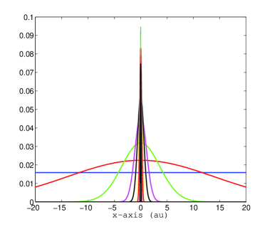
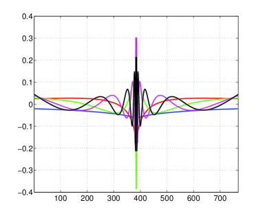
Figure 2.1 displays several vectors of the canonical and Tucker tensor representations for a single Newton kernel along -axis from a set . Symmetry of the tensor implies that the canonical vectors and corresponding to and -axes, respectively, are of the same shape as . It is clearly seen that there are canonical/Tucker vectors representing the long-, intermediate- and short-range contributions to the total electrostatic potential. This interesting feature will be also recognized for the low-rank lattice sum of potentials (see §3.2).
Table 2.1 presents CPU times (sec) for generating a canonical rank- tensor approximation of the single Newton kernel over 3D Cartesian grid, corresponding to Matlab implementation on a terminal of the 8 AMD Opteron Dual-Core processor. The corresponding mesh sizes are given in ngstroms. We observe a logarithmic scaling of the canonical rank in the grid size , while the maximal Tucker rank has the tendency to decrease for larger . The compression rate for the grid , that is the ratio for the canonical format and for the Tucker format are of the order of and , respectively.
| grid size | |||||
|---|---|---|---|---|---|
| mesh size | |||||
| Time (Canon.) | |||||
| Canonical rank | |||||
| Time (C2T) | |||||
| Tucker rank |
Notice that the low-rank canonical/Tucker approximation of the tensor is the problem independent task, hence the respective canonical/Tucker vectors can be precomputed at once on large enough 3D grid, and then stored for the multiple use. The storage size is bounded by or .
2.2 Low-rank representation for the general class of kernels
Along with Coulombic systems corresponding to , the tensor approximation described above can be also applied to a wide class of commonly used long-range kernels in , for example, to the Slater, Yukawa, Lennard-Jones or Van der Waals and dipole-dipole interactions potentials defined as follows,
The simplified version of the Lennard-Jones potential is the so-called Buckingham function
The electrostatic potential energy for the dipole-dipole interaction due to Van der Waals forces is defined by
The quasi-optimal low-rank decompositions based on the -quadrature approximation to the Laplace transforms of the above mentioned functions can be rigorously proven for a wide class of generating kernels. In particular, the following Laplace (or Laplace-Gauss) integral transforms [48] with a parameter can be applied for the -quadrature approximation of the above mentioned functions,
| (2.8) | |||||
| (2.9) | |||||
| (2.10) | |||||
| (2.11) |
combined with the subsequent substitution of a parameter by the appropriate function , usually by using an additive representation . In the cases (2.11) () and (2.10) the convergence rate for the -quadrature approximations of type (2.3) has been considered in [4, 5] and later analyzed in more detail in [16, 19]. The case of the Yukawa and Slater kernel has been investigated in [28, 29]. The exponential error bound for the general transform (2.11) can be derived by minor modifications of the above mentioned results.
Remark 2.2
The idea behind the low-rank tensor representation for a sum of spherically symmetric potentials on a 3D lattice can be already recognized on the continuous level by introducing the Laplace transform of the generating kernel. For example, in representation (2.9) with the particular choice , that is given by (2.10), we can set up , i.e. , (), and apply the -quadrature approximation as in (2.2)-(2.3),
| (2.12) |
Now the simple sum on a rectangular lattice of width ,
can be represented by the agglomerated integral transform
| (2.13) |
where the integrand is separable. Representation (2.13) indicates that applying the same quadrature approximation to the lattice sum integral (2.13) as that for the single kernel (2.12) will lead to the decomposition of the total sum of potentials with the same canonical rank as for the single one.
In the following, we construct the low-rank canonical and Tucker decompositions of the lattice sum of interaction potentials discretized on the fine representation 3D-grid and applied to the general class of kernel functions and more general configuration of a lattice.
3 Tucker decomposition for lattice sum of potentials
3.1 Direct tensor sum for a moderate number of arbitrarily distributed potentials
In this paragraph, we recall the direct tensor summation of the electrostatic potentials for a moderate number of arbitrarily distributed sources as introduced in [24, 25].
The basic example in electronic structure calculations is concerned with the nuclear potential operator describing the Coulombic interaction of electrons with the nuclei in a molecular system in a box corresponding to the choice . We consider a function describing the interaction potential of several nuclei in a computational box ,
| (3.1) |
where is the (moderate) number of nuclei in , and , , represent their coordinates and “charges“, respectively. We are interested in the low-lank representation of the projected tensor along the line of §2.1,
Similar to [25, 26], we first approximate the non-shifted kernel on the auxiliary extended box in the canonical format by its projection onto the basis set of piecewise constant functions as described in §2.1, and defined on a uniform tensor grid with the mesh size , with embedding . This defines the ”reference“ rank- canonical tensor as above
| (3.2) |
For ease of exposition, we assume that each nuclei coordinate is located exactly222Our numerical scheme is designed for nuclei positioned arbitrarily in the computational box where approximation error of order is controlled by choosing large enough grid size . Indeed, computational cost enables us usage of fine grids of size in Matlab implementation, yielding mesh size , i.e. is of the order of the atomic radii. This grid-based tensor calculation scheme for the nuclear potential operator was tested numerically in molecular calculations [24], where it was compared with the results of analytical evaluation of the same operator from benchmark quantum chemical packages. at certain grid-point , with some . Now we are in a position to introduce the rank- shift-and-windowing operator
via
| (3.3) |
With this notation, the projected tensor approximating the total electrostatic potentials in is represented by a direct sum of low-rank canonical tensors
| (3.4) |
where every rank- canonical tensor is thought as a sub-tensor of the reference tensor obtained by its shifting and restriction (windowing) onto the grid in the computational box . Here a shift from the origin is specified according to the coordinates of the corresponding nuclei, , counted in the -units.
For example, the electrostatic potential centered at the origin, i.e. with , corresponds to the restriction of onto the initial computational box , i.e. onto the index set (assume that is even)
The projected tensor approximating the function in (3.1) is represented as a canonical tensor with the rough bound on its rank , where . However, our numerical tests for moderate size molecules indicate that the tensor ranks of the -term canonical sum representing can be considerably reduced, such that . This rank optimization can be implemented, for example, by the multigrid version of the canonical rank reduction algorithm, canonical-Tucker-canonical, based on RHOSVD approximation [32]. The resultant canonical tensor will be denoted by .
Along the same line, the direct sum in the Tucker format can be represented by using shift-and-windowing projection of the ”reference” rank- Tucker tensor
| (3.5) |
approximating the Newton kernel in the Tucker format,
| (3.6) |
As in the case of canonical decomposition, the rank reduction procedure based on ALS-type iteration applies to the sum of Tucker tensors, , resulting in the optimized Tucker tensor with the reduced rank parameter .
Summary 3.1
We summarize that a sum of arbitrarily located potentials in a box can be calculated by a shift-and-windowing tensor operation applied to the low-rank canonical/Tucker representations for the ”reference“ tensor. Usually in electronic structure calculations the -rank of the resultant tensor sum can be reduced to the quasi-optimal level of the same order as the rank of a single ”reference“ tensor.
The grid-based representation of a sum of electrostatic potentials given by in the form of a tensor in the canonical or Tucker format enables its easy projection to some separable basis set, like GTO-type atomic orbital basis, polynomials or plane waves.
The following example illustrates that calculation of the Galerkin matrix in the Tucker tensor format (cf. [24, 25] for the case of canonical representations) is reduced to a combination of 1D Hadamard and scalar products [32]. Suppose, for simplicity, that the basis set is represented by rank- canonical tensors, , representing the basis set, i.e. with the canonical vectors , associated with mode , and , where is the number of basis functions (vectors).
Suppose that a sum of potentials in a box, , given by (3.1), is considered as a multiplicative potential in certain operator (say, the Hartree-Fock/Kohn-Sham Hamiltonian). Given the Tucker tensor approximation to in form (3.6), with the optimized rank parameters , then its projection onto the given basis set is represented by the Galerkin matrix, , whose entries are calculated (approximated) by the simple tensor operations,
| (3.7) |
where
denotes the Hadamard (entrywise) product of rank- tensors. The expression (3.7) can be calculated in terms of 1D Hadamard and scalar products with linear complexity .
Similar to the case of Galerkin projection onto the well separable basis set, many other tensor operations on the canonical/Tucker representations of can be calculated with the linear cost .
Finally, we notice that the approximation error caused by a separable representation of the nuclear potential is controlled by the rank parameter , where mildly depends on the number of nuclei in a system. The exponential convergence of the canonical/Tucker approximation in the rank parameters allows us the optimal choice adjusting the complexity bound , almost independent on .
3.2 Assembled lattice sums in a box by using the Tucker format
In this paragraph, we introduce the efficient scheme for fast agglomerated summation on a lattice in a box in the Tucker tensor format applied to rather general interaction potentials.
Given the potential sum in the reference unit cell , of size , we consider an interaction potential in a bounded box
consisting of a union of unit cells , obtained by a shift of along the lattice vector , where , such that for with and . In the following, for ease of exposition, we consider a lattice of equal sizes . By the construction , where is the mesh-size that is the same for all spacial variables. Figure 3.1 illustrates an example of a 3D lattice structure in a box.
The potential , for is obtained by summation over all unit cells in ,
| (3.8) |
Note that conventionally this calculation is performed at each of unit cells , , on the rectangular lattice, which presupposes substantial numerical costs at least of the order of . The presented approach applies not only to the complete rectangular lattice, but remains efficient in the case of defected lattices and for more complicated symmetries. It allows to essentially reduce these costs to linear scaling in .
Let be the uniform grid on with the same mesh-size as above, and introduce the corresponding space of piecewise constant basis functions of the dimension . In this construction we have . In the case of canonical sums, we simply follow [26], and employ, similar to (3.2), the rank- ”reference“ tensor defined on the larger auxiliary box by scaling with a factor of ,
| (3.9) |
Along the same line as in (3.5), we introduce the rank- ”reference“ Tucker tensor defined on the auxiliary domain .
The next theorem generalizes Theorem 3.1 in [26] to the case of general function in (3.8) as well as to the case of Tucker tensor decompositions. It proves the storage and numerical costs for the lattice sum of single potentials (i.e. corresponding to the choice , and in (3.8)), each represented by a rank- canonical or rank- Tucker tensors. In what following the windowing operator specifies a shift by the lattice vector .
Theorem 3.2
(A) Given the rank- canonical ”reference” tensor (3.9) approximating the potential . The projected tensor of the interaction potential, , representing the full lattice sum over cells can be presented by the rank- canonical tensor ,
| (3.10) |
The numerical cost and storage size are estimated by and , respectively, where is the univariate grid size.
(B) Given the rank- ”reference“ Tucker tensor , see (3.5), approximating the potential function . The rank- Tucker approximation of a lattice-sum tensor can be computed in the form
| (3.11) |
The numerical cost and storage size are estimated by and , respectively.
Proof. Conventionally, we fix the index in (3.8), set and , and consider only the second sum defined on the complete domain ,
| (3.12) |
Then the projected tensor representation of takes the form
where the 3D shift vector is defined by . Taking into account the rank- separable representation of the -windowing operator (tracing onto window),
we rewrite the above summation as
| (3.13) |
To reduce the large sum over the full 3D lattice, we use the following property of a sum of canonical tensors, , with equal ranks and with two coinciding factor matrices, say for : the concatenation in the remaining mode can be reduced to a pointwise summation of the respective canonical vectors,
| (3.14) |
while the first two mode vectors remain unchanged, , . This preserves the same rank parameter for the resulting sum. Notice that for each fixed the inner sum in (3.13) satisfies the above property. Repeatedly applying this property to a large number of canonical tensors, the 3D-sum (3.13) is reduced to a rank- tensor obtained by 1D summations only,
The numerical cost are estimated by using the standard properties of canonical tensors.
In the case of Tucker representation we apply the similar argument to obtain
Simple complexity estimates complete the proof.
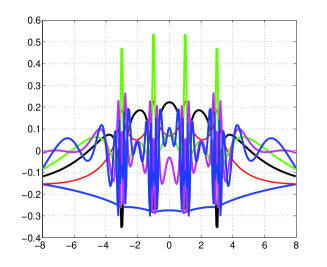
Figure 3.2 illustrates the shape of several Tucker vectors obtained by assembling vectors along -axis. It can be seen that assembled Tucker vectors accumulate simultaneously the contributions of all single potentials involved in the total sum. Note that the assembled Tucker vectors do not preserve the initial orthogonality of directional vectors . In this case the simple Gram-Schmidt orthogonalization can be applied.
Remark 3.3
In the general case , the weighted summation over charges leads to the rank- canonical tensor representation on the ”reference” domain , which can be used to obtain the rank- representation of a sum in the whole lattice
| (3.15) |
Likewise, the rank- Tucker approximation of a tensor can be computed in the form
| (3.16) |
The next remark generalizes the basic construction to the case of non-uniformly spaced rectangular lattices.
Remark 3.4
The previous construction applies to the uniformly spaced positions of charges. However, the agglomerated tensor summation method in both canonical and Tucker formats applies with slight modification of the windowing operator to a non-equidistant tensor lattice. Such lattice sums could not be treated by the traditional Ewald summation methods based on the FFT transform.
| Time | ||||
|---|---|---|---|---|
Both the Tucker and canonical tensor representations (3.11) and (3.10) reduce dramatically the numerical costs and storage consumptions. Table 3.1 illustrates complexity scaling for computation of lattice sum in the Tucker format, where the grid-size is given by with . These results confirm our theoretical estimates.
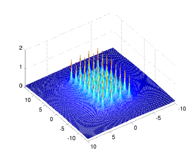
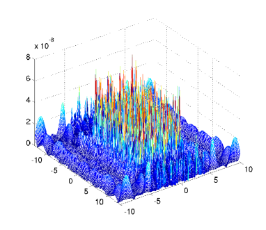
Figure 3.3 shows the sum of Newton kernels on a lattice and the respective Tucker summation error achieved on the large 3D representation grid with the rank Tucker tensor. The spacial mesh size is about atomic units ( Å).
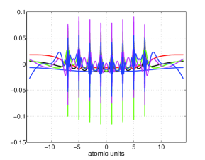
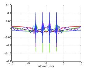
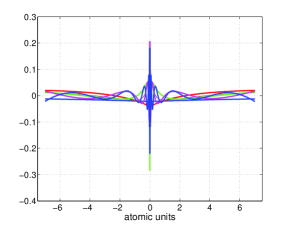
Figure 3.4 represents the Tucker vectors obtained from the canonical-to-Tucker (C2T) approximation of the assembled canonical tensor sum of potentials on a lattice. In this case the Tucker vectors are orthogonal.
4 Potential sums on defected lattice
4.1 Problem setting
For lattice sums on the perfect rectangular geometries the resultant canonical and Tucker tensors are proven to inherit exactly the same rank parameters as those for the single ”reference“ tensor. In the case of lattices with defects, say, vacancies or impurities, the tensor rank of agglomerated sums in both canonical and Tucker formats may increase dramatically. In such cases the rank reduction procedure is required.
In this section, we analyze the assembled summation of Tucker/canonical tensors on the defected lattices in the algebraic framework as follows. Denote the perturbed Tucker tensor by . Let us introduce a set of -indices on the lattice, , where the unperturbed Tucker tensor initially given by summation over the full rectangular lattice (3.11) is perturbed (defected) at positions associated with by the Tucker tensor (), given by,
| (4.1) |
Without loss of generality, all Tucker tensors , (), can be assumed orthogonal.
Now the perturbed Tucker tensor is obtained from the non-perturbed one, , by adding a sum of all defects , ,
| (4.2) |
which implies the upper rank estimates for best Tucker approximation of ,
If the number of perturbed cells, , is large enough, the numerical computations with the Tucker tensor of rank becomes prohibitive and the rank reduction procedure is required.
In the case of lattice sum in the Tucker format, we propose the generalization to the RHOSVD algorithm, that applies directly to a large sum of Tucker tensors. In this way the initial RHOSVD algorithm in [32] can be viewed as the special case of generalized RHOSVD scheme now applied to a sum of rank-one Tucker tensors. The stability of the new rank reduction method can be proven under mild assumptions on the ”weak orthogonality“ of the Tucker tensors representing defects in the lattice sum. The numerical complexity of the generalized RHOSVD algorithm scales only linearly in the number of vacancies.
We use the similar notation to describe the summation of canonical tensors on defected lattices. The non-perturbed canonical tensor given by (3.10) is substituted by a sum of canonical tensors representing the expected perturbations,
| (4.3) |
with the upper rank estimate for best canonical approximation of the perturbed canonical tensor ,
| (4.4) |
Again, the rank reduction procedure is normally required.
4.2 Defected lattice sum of canonical tensors
We consider a sum of canonical tensors on a lattice with defects located at sources. In accordance with (4.3) - (4.4), the canonical rank of the resultant tensor may increase at a factor of . The effective rank of the perturbed sum may be reduced by using the RHOSVD approximation via Can Tuck Can algorithm, proposed in [32]. This approach basically provides the compressed tensor with the canonical rank quadratically proportional to those of the respective Tucker approximation to the sum with defects. For the readers convenience, in Appendix, we recall the error estimate for RHOSVD approximation to sums of canonical tensors [32].
In what follows, we discuss the stability conditions for RHOSVD approximation and their applicability in the summation on spherically symmetric interaction potentials. Given a rank parameter , we denote by
| (4.5) |
the canonical tensor with normalized vectors () that is defined by the side-matrices , obtained by concatenation of the corresponding canonical vectors in (4.5). The minimal parameter in (4.5) is called the rank (or canonical rank) of a tensor. The representation (4.5) can be written as the rank- Tucker tensor by introducing the diagonal Tucker core tensor such that except when with (),
| (4.6) |
Given the rank parameter . To define the reduced rank- HOSVD type Tucker approximation to the tensor in (4.5), we set and suppose for definiteness that , so that SVD of the side-matrix is given by
with the orthogonal matrices , and , . Given rank parameters , introduce the truncated SVD of the side-matrix , , (), where and , , represent the orthogonal factors being the respective sub-matrices in the SVD factors of .
Definition 4.1
The stability of RHOSVD approximation is formulated in the following assertion.
Lemma 4.2
Let decomposition (4.5) satisfy the stability condition
| (4.7) |
then the quasi-optimal RHOSVD approximation is robust in the relative norm
where () denote the truncated singular values.
Proof. The proof is a simple consequence of the general error estimate (6.3).
The stability condition (4.7) is fulfilled, in particular, if
(a) All canonical vectors in (4.5) are non-negative that is the case for -quadrature based approximations to Green’s kernels based on integral transforms (2.8) - (2.11), since .
(b) The partial orthogonality of the canonical vectors holds, i.e. rank- tensors () are mutually orthogonal. We refer to [34] for various definitions of orthogonality for canonical tensors.
4.3 Summation on defected lattice in the Tucker tensor format
In the case of Tucker sum (4.2) we define the agglomerated side matrices by concatenation of the directional side-matrices of individual tensors , ,
| (4.8) |
Given the rank parameter , introduce the truncated SVD of ,
where . Here instead of fixed rank parameter the truncation threshold can be chosen.
Now items (a) - (d) in Theorem 6.1 can be generalized to the case of Tucker tensors. In particular, the stability criteria for RHOSVD approximation as in Lemma 4.2 allows natural extension to the case of generalized RHOSVD approximation applied to a sum of Tucker tensors in (4.2).
The following theorem provides the error estimate for the generalized RHOSVD approximation converting a sum of Tucker tensors to a single Tucker tensor with fixed rank bounds, or subject to the given tolerance .
Theorem 4.3
(Tucker-Sum-to-Tucker)
Given a sum of Tucker tensors (4.2) and the rank truncation
parameter .
(a) Let
be the singular values of the -mode side-matrix
() defined in (4.8).
Then the generalized RHOSVD approximation
obtained by the projection of onto the dominating singular
vectors of the Tucker side-matrices,
,
exhibits the error estimate
| (4.9) |
(b) Assume the stability condition for the sum (4.2),
then the generalized RHOSVD approximation provides the quasi-optimal error bound
Proof. Proof of item (a) is similar to those for Theorem 6.1, presented in [32]. Item (b) follows from (4.9) taking into account the stability condition.
The resultant Tucker tensor can be considered as the initial guess for the ALS iteration to compute best Tucker -approximation of a sum of Tucker tensors.
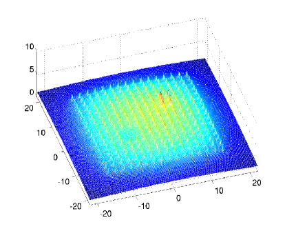
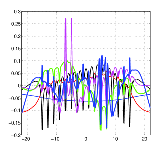
Figure 4.1 (left) visualizes result of assembled Tucker summation of 3D grid-based Newton potentials on a lattice, with a vacancy and impurity, each of lattice size. Figure 4.1 (right) shows the corresponding Tucker vectors along -axis. These vectors clearly represent the local shape of vacancies and impurities.
4.4 Summation over non-rectangular lattices
In many practically interesting cases the physical lattice may have non-rectangular geometry that does not fit exactly the tensor-product structure of the canonical/Tucker data arrays. For example, the hexagonal or parallelepiped type lattices as well as their combination can be considered. The case study of many particular classes of geometries is beyond the scope of our paper. Instead, we formulate the main principles on how to apply tensor summation methods to certain classes of non-rectangular geometries and give a few examples demonstrating the required (minor) modifications of the basic agglomerated summation schemes described above.
It is worth to note that most of interesting lattice structures (say, arising in crystalline modeling) inherit a number of spacial symmetries which allow, first, to classify and then simplify the computational schemes for each particular case of symmetry. In this concern, we consider the following classes of lattice topologies which can be efficiently treated by our tensor summation techniques:
-
(A)
The target lattice can be split into the union of several (few) sub-lattices, , such that each sub-lattice allows a 3D rectangular grid-structure.
-
(B)
The 3D lattice points belong to the rectangular tensor grid in two spatial coordinates, but they violate the tensor structure in the third variable (say, parallelogram type grids).
-
(C)
The 3D lattice points belong to the tensor grid in one of spatial coordinate, but they may violate the rectangular tensor structure in the remaining couple of variables.
-
(D)
Defects in the target lattice are distributed over rectangular sub-lattices (clusters) represented on several coarser scales (multi-level tensor lattice sum).
In case (A) the agglomerated tensor summation algorithms apply independently to each rectangular sub-lattice , and then the target tensor is obtained as a direct sum of tensors associated with , supplemented by the subsequent rank reduction procedure. The example of such a geometry is given by hexagonal grid presented in Figure 4.3, left ( section of the D lattice, that is rectangular in -direction), which can be split into a union of two rectangular sub-lattices (red) and (blue). Another example is a lattice with -shape boundary. In this case the maximal rank does not exceed the multiple of and the rank of a single reference Tucker tensor.
In case (B) the tensor summation applies only in two indices while a sum in the remaining third index is treated directly. This leads to the increase of directional rank proportionally to the 1D size of the lattice, , hence requiring the subsequent rank reduction procedures described in §4.2 and §4.3. This may lead to the higher computational complexity of the summation. An example of such a structure is the parallelogram-type lattice shown in Figure 4.3, right (orthogonal projection onto plane).
In case (C) the agglomerated summation can be performed only in one index, supplemented by the direct summation in the remaining indices. The total rank then increases proportionally to , making the subsequent rank optimization procedure indispensable. However, even in this worst case scenario the asymptotic complexity of the direct summation shall be reduced on the order of magnitude in from to due to the benefits of ”one-way” tensor summation.
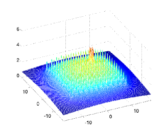
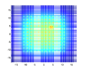
Case (D) can be treated by successive application of the canonical/Tucker tensor summation algorithm at several levels of defects location. Figure 4.4 represent the result of assembled canonical summation of 3D grid-based Newton potentials on a lattice , with an impurity of size that does not fit the location of lattice points. Since the impurity potentials are determined on the same fine representation grid, the difference in inter-potential distances does not influence on the numerical treatment of the defects. In the case of many non-regularly distributed defects the summation should be implemented in the Tucker format with the subsequent rank truncation.
Figure 4.5 (left) visualizes the result of assembled canonical summation of 3D grid-based Newton potentials on a lattice , with regularly positioned vacancies (two-level lattice). Figure 4.5 represents the result of assembled canonical summation of the Newton potentials on -shaped (left) and -shaped (right) sub-lattices of the lattice (two-level step-type geometry). In all these cases the total tensor rank does not exceed the double rank of the single reference potential since all vacancies are located on tensor sub-lattice of the target lattice.
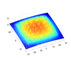
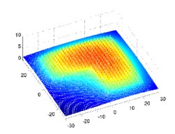
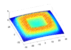
We summarize that in all cases (A) - (D) classified above the tensor summation approach cab be gainfully applied. The overall numerical cost may depend on the geometric structure and symmetries of the system under consideration since violation of the tensor-product rectangular structure of the lattice may lead to the increase in the Tucker/canonical rank. This is clearly observed in the case of moderate number of defects distributed randomly. In all such cases the RHOSVD approximation combined with the ALS iteration serves for the robust rank reduction in the Tucker format.
5 Conclusions
In this paper we presented the fast rank-structured tensor method for the efficient grid-based summation of long-range potentials on lattices with vacancies and defects, as well as in the presence of non-rectangular geometries. It is shown that summation of potentials on perturbed lattices by using the Tucker/canonical tensor formats can be performed in operations that improves dramatically the cost by the standard methods.
All computational 3D data are presented on the one common fine grid by low-rank tensors in , that allows the simultaneous approximation with guaranteed precision of all singular kernel functions involved in the summation. In case of unperturbed lattice, both the canonical and Tucker ranks of the resultant tensor sum remains the same as for the individual reference potential.
Calculation of the potential sum on defected lattices is performed in an algebraic way, by using summation rules for tensors in the canonical or Tucker formats, which lead to increase in the Tucker or canonical ranks of the resultant tensor. The rank truncation for the overall potential sum is based on the canonical-to-Tucker or Tucker-sum-to-Tucker transform via the reduced HOSVD approximation. The stability conditions for such kind of approximation have been analyzed.
The presented approach yields enormous reduction in storage and computing time. Numerical examples illustrate the rank bounds and asymptotic complexity of the tensor summation method in both canonical and Tucker data formats in the agreement with theoretical predictions. Summation of millions of potentials on a finite 3D lattice is performed in seconds in Matlab implementation.
This scheme can be applied to a number of potentials including the Newton, Slater, Yukawa, Lennard-Jones, Buckingham and dipole-dipole kernel functions. The assembled tensor summation approach is well suited for further applications in electronic and molecular structure calculations of large lattice-structured compounds, see [27], as well as in various computational problems for many-particle systems. In particular, it is can be efficient for calculation of electronic properties of large finite crystalline systems like quantum dots, which are intermediate between bulk (periodic) systems and discrete molecules.
6 Appendix: Canonical-to-Tucker approximation
In Appendix we present the error estimate for the RHOSVD approximation by the so-called Canonical-to-Tucker scheme [32]. Let us denote by the so-called Grassman manifold that is a factor space with respect to all possible rotations to the Stiefel manifold of orthogonal matrices,
Denote by the set of rank- Tucker tensors.
Theorem 6.1
(Canonical to Tucker approximation, [32]).
(a) Let be given by (4.5). Then the minimization problem
| (6.1) |
is equivalent to the ual maximization problem over the Grassman manifolds ,
| (6.2) |
where (), and .
(b) The compatibility condition being the -mode side-matrix, ensures the solvability of (6.2). The maximizer is given by orthogonal matrices , which can be computed by ALS Algorithm with the initial guess chosen as the reduced HOSVD approximation of given by , see Definition 4.1.
(c) Precomputed matrices , the minimizer in (6.1) is then calculated by the orthogonal projection
where the core tensor can be represented in the rank- canonical format
(d) Let be the singular values of the -mode side-matrix (). Then the reduced HOSVD approximation exhibits the error estimate
| (6.3) |
References
- [1] C. Bertoglio, and B.N. Khoromskij. Low-rank quadrature-based tensor approximation of the Galerkin projected Newton/Yukawa kernels. Comp. Phys. Communications, 183(4) (2012) 904–912.
- [2] Bloch, André, ”Les theoremes de M. Valiron sur les fonctions entieres et la theorie de l’uniformisation”. Annales de la faculte des sciences de l’universite de Toulose 17 (3): 1-22 (1925). ISSN 0240-2963.
- [3] Boys, S. F., Cook, G. B., Reeves, C. M. and Shavitt, I. (1956). Automatic Fundamental Calculations of Molecular Structure. Nature, 178: 1207-1209.
- [4] D. Braess. Nonlinear approximation theory. Springer-Verlag, Berlin, 1986.
- [5] D. Braess. Asymptotics for the Approximation of Wave Functions by Exponential-Sums. J. Approx. Theory, 83: 93-103, (1995).
- [6] E. Cancés, V. Ehrlacher, and Y. Maday. Periodic Schrödinger operator with local defects and spectral pollution. SIAM J. Numer. Anal. v. 50, No. 6, pp. 3016-3035.
- [7] E. Cancés and C. Le Bris. Mathematical modeling of point defects in materials science. Math. Methods Models Appl. Sci. 23 (2013) 1795-1859.
- [8] T. Darten, D. York and L. Pedersen. Particle mesh Ewald: An method for Ewald sums in large systems. J. Chem. Phys., 98, 10089-10091, 1993.
- [9] L. De Lathauwer, B. De Moor, J. Vandewalle. A multilinear singular value decomposition. SIAM J. Matrix Anal. Appl., 21 (2000) 1253-1278.
- [10] M. Deserno and C. Holm. How to mesh up Ewald sums. I. A theoretical and numerical comparison of various particle mesh routines. J. Chem. Phys., 109(18): 7678-7693, 1998.
- [11] S.V. Dolgov. Tensor-product methods in numerical simulation of high-dimensional dynamical problems., University of Leipzig, Dissertaion, 2014. http://nbn-resolving.de/urn:nbn:de:bsz:15-qucosa-151129
- [12] Sergey Dolgov, Boris N. Khoromskij, Alexander Litvinenko, and Hermann G. Matthies. Computation of the Response Surface in the Tensor Train data format. E-preprint arXiv:1406.2816, 2014.
- [13] R. Dovesi, R. Orlando, C. Roetti, C. Pisani, and V.R. Sauders. The Periodic Hartree-Fock Method and its Implementation in the CRYSTAL Code. Phys. Stat. Sol. (b) 217, 63 (2000).
- [14] V. Ehrlacher, C. Ortner, and A. V. Shapeev. Analysis of boundary conditions for crystal defect atomistic simulations. e-prints ArXiv:1306.5334, 2013.
- [15] Ewald P.P. Die Berechnung optische und elektrostatischer Gitterpotentiale. Ann. Phys 64, 253 (1921).
- [16] I.P. Gavrilyuk, W. Hackbusch and B.N. Khoromskij. ata-Sparse Approximation to a Class of Operator-Valued Functions. Math. Comp. 74 (2005), 681-708.
- [17] L. Grasedyck, D. Kressner and C. Tobler. A literature survey of low-rank tensor approximation techniques. arXiv:1302.7121v1, 2013.
- [18] L. Greengard and V. Rochlin. A fast algorithm for particle simulations. J. Comp. Phys. 73 (1987) 325.
- [19] W. Hackbusch and B.N. Khoromskij. Low-rank Kronecker product approximation to multi-dimensional nonlocal operators. Part I. Separable approximation of multi-variate functions. Computing 76 (2006), 177-202.
- [20] W. Hackbusch, and R. Schneider. Tensor Spaces and Hierarchical Tensor Representations. In: Lecture Notes in Computer Science and Engineering, 102, S. Dahlke, W. Dahmen, et al. eds., p. 237-262, Springer, 2014.
- [21] T. Helgaker, P. Jørgensen, and J. Olsen. Molecular Electronic-Structure Theory. Wiley, New York, 1999.
- [22] Philippe H. Hünenberger. Lattice-sum methods for computing electrostatic interactions in molecular simulations. CP492, L.R. Pratt and G. Hummer, eds., 1999, American Institute of Physics, 1-56396-906-8/99.
-
[23]
Venera Khoromskaia.
Numerical Solution of the Hartree-Fock Equation by Multilevel Tensor-structured methods.
Dissertation, TU Berlin, 2010.
http://opus4.kobv.de/opus4-tuberlin/frontdoor/index/index/docId/2780 - [24] V. Khoromskaia, D. Andrae, and B.N. Khoromskij. Fast and accurate 3D tensor calculation of the Fock operator in a general basis. Comp. Phys. Communications, 183 (2012) 2392-2404.
- [25] V. Khoromskaia. Black-box Hartree-Fock solver by tensor numerical methods. Comp. Meth. in Applied Math., Vol. 14 (2014) No.1, pp. 89-111.
- [26] V. Khoromskaia and B. N. Khoromskij. Grid-based lattice summation of electrostatic potentials by assembled rank-structured tensor approximation. Comp. Phys. Communications, 185 (2014), pp. 3162-3174.
- [27] V. Khoromskaia, and B.N. Khoromskij. Tensor Approach to Linearized Hartree-Fock Equation for Lattice-type and Periodic Systems. E-preprint arXiv:1408.3839, 2014 (submitted).
- [28] B.N. Khoromskij, Structured Rank- Decomposition of Function-related Tensors in . Comp. Meth. in Applied Math., 6 (2006), 2, 194-220.
- [29] B.N. Khoromskij. On Tensor Approximation of Green Iterations for Kohn-Sham Equations. Computing and Visualization in Sci., 11: 259-271 (2008).
- [30] B.N. Khoromskij. -Quantics Approximation of - Tensors in High-Dimensional Numerical Modeling. Constructive Approx. 34 (2011) 257–280. (Preprint 55/2009 MPI MiS, Leipzig 2009.)
- [31] B. N. Khoromskij and V. Khoromskaia. Low Rank Tucker Tensor Approximation to the Classical Potentials. Central European J. of Math., 5(3) 2007, 1-28.
- [32] B.N. Khoromskij and V. Khoromskaia. Multigrid tensor approximation of function related multi-dimensional arrays. SIAM J. Sci. Comp. 31(4) (2009) 3002-3026.
- [33] Boris N. Khoromskij. Tensor Numerical Methods for High-dimensional PDEs: Basic Theory and Initial Applications. E-preprint arXiv:1408.4053, 2014. ESAIM: Proceedings 2014 (to appear).
- [34] T. Kolda. Orthogonal tensor decompositions. SIAM J. Matrix Anal. Appl. 23 (2001) 243-255.
- [35] T.G. Kolda and B.W. Bader. Tensor Decompositions and Applications. SIAM Rev. 51(3) (2009) 455–500.
- [36] K.N. Kudin, and G.E. Scuseria, Revisiting infinite lattice sums with the periodic Fast Multipole Method, J. Chem. Phys. 121, 2886-2890 (2004).
- [37] S. A. Losilla, D. Sundholm, J. Juselius. The direct approach to gravitation and electrostatics method for periodic systems. J. Chem. Phys. 132 (2) (2010) 024102.
- [38] M. Luskin, C. Ortner, and B. Van Koten. Formulation and optimization of the energy-based blended quasicontinuum method. Comput. Methods Appl. Mech. Engrg., 253, 2013.
- [39] I.V. Oseledets. Tensor-train decomposition. SIAM J. Sci. Comp., 33(5), 2011, pp. 2295-2317.
- [40] I.V. Oseledets. DMRG approach to fast linear algebra in TT format. CMAM, 11, 3, 382-393, 2011.
- [41] C. Pisani, M. Schütz, S. Casassa, D. Usvyat, L. Maschio, M. Lorenz, and A. Erba. CRYSCOR: a program for the post-Hartree-Fock treatment of periodic systems. Phys. Chem. Chem. Phys., 2012, 14, 7615-7628.
- [42] E.L. Pollock, and Jim Glosli. Comments on , , and the Ewald method for large periodic Coulombic systems. Computer Phys. Communication 95 (1996), 93-110.
- [43] D. V. Savostyanov, S. V. Dolgov, J. M. Werner and I. Kuprov. Exact NMP simulation of protein-size spin systems using tensor train formalism. Phys. Rev. B 90, 085139, 2014.
- [44] U. Schollwöck. The density-matrix renormalization group in the age of matrix product states, Ann.Phys. 326 (1) (2011) 96-192.
- [45] F. Stenger. Numerical methods based on Sinc and analytic functions. Springer-Verlag, 1993.
- [46] A.Y. Toukmaji, and J. Board Jr. Ewald summation techniques in perspective: a survey. Computer Phys. Communication 95 (1996), 73-92.
- [47] Elena Voloshina, Denis Usvyat, Martin Schütz, Yuriy Dedkov and Beate Paulus. On the physisorption of water on graphene: a CCSD(T) study. Phys. Chem. Chem. Phys., 2011, 13, 12041-12047.
- [48] E. Zeidler. Oxford User’s Guide to Mathematics. Oxford University Press, 2003.