The local phase transitions of the solvent in the neighborhood of a solvophobic polymer at high pressures

Abstract

We investigate local phase transitions of the solvent in the neighborhood of a solvophobic polymer chain which is induced by a change of the polymer-solvent repulsion and the solvent pressure in the bulk solution. We describe the polymer in solution by the Edwards model, where the conditional partition function of the polymer chain at a fixed radius of gyration is described by a mean-field theory. The contributions of the polymer-solvent and the solvent-solvent interactions to the total free energy are described within the mean-field approximation. We obtain the total free energy of the solution as a function of the radius of gyration and the average solvent number density within the gyration volume. The resulting system of coupled equations is solved varying the polymer-solvent repulsion strength at high solvent pressure in the bulk. We show that the coil-globule (globule-coil) transition occurs accompanied by a local solvent evaporation (condensation) within the gyration volume.

I Introduction

In 2002 ten Wolde and David Chandler proposed a very elegant idea Chandler_2002 stating that a hydrophobic polymer chain immersed in an aqueous medium, can undergo a coil-globule transition when in a neighborhood of the polymer a surface dewetting transition occurs.

The authors speculated, based on the results of computer simulations, that this effect is reminiscent of the first-order phase transition. It should be noted that this statement amounts to proposing a fundamentally new mechanism of the polymer collapse, which is distinct from the standard mechanism adopted in statistical mechanics of macromolecules. As is well known from the polymer statistical mechanics, when the solvent becomes poorer, the polymer coil shrinks leading eventually to a collapse of the polymer coil DeGennes ; Grosberg_Khohlov .

To describe the above mentioned mechanism within a theory it is therefore necessary to take the solvent explicitly into account. However, most theoretical models describe the solvent only implicitly Edwards_1 ; Edwards_2 ; Birshtein_1 ; Birshtein_2 ; Moore ; Lifshitz ; Lifshitz_Grosberg ; deGennes_collaps ; Muthukumar ; Sanchez ; Kholodenko ; Grosberg1 ; Grosberg2 ; Grosberg3 ; Grosberg4 ; Khohlov ; Khohlov_2 , i.e. its influence on the macromolecule is taken into account through an effective monomer-monomer interaction. Such an approach simplifies the model, however the details of the solvent behavior – in particular phase transitions in the bulk solution, heterogeneity of the solvent near the polymer chain, and the dependence of the solvent quality on the pressure – are not taken into account. At present only few examples exist considering the solvent explicitly.

In the pioneering works of Flory and Schultz Flory_Schultz (mean-field theory), de Gennes and Brochard deGennes2 (scaling approach) and the works of Vilgis and co-authors Vilgis ; Vilgis_Dua ; Dua (path integral methodology) describing the conformational behavior of a polymer chain in a vicinity of the binary mixture critical point the solvent has been taken into account explicitly. The authors in Lifshitz_Grosberg briefly discussed the influence of the solvent on the spatial structure of the globule. In Erukhimovich_JETP a field-theoretical approach has been adopted to investigate the density of the globule in a critical solvent.

In the work of Matsuyama and Tanaka Tanaka the conformational phase transition of an isolated polymer chain has been approached. The chain was allowed to form physical bonds with explicitly present solvent molecules. On the basis of a Flory mean-field type theory, a formula for the temperature dependence of the expansion factor of the chain has been derived. The formation of physical bonds between the polymer and the solvent molecules was shown to cause a re-entrant conformational change between a coiled and a globular state when the temperature was varied. Tanaka et al Tanaka2 considered a model for poly(N-isopropylacrylamide) chain in a water - methanol mixture on the basis of statistical mechanics. The model included a competitive water-polymer and methanol-polymer hydrogen bond formation. The obtained mean squared end-to-end distance has been compared with experiments. In the work Tamm have classified the various types of the coil-globule transition of a polymer chain in an associating solvent taking into account the microscopic nature of such the solvent.

Unfortunately, most theoretical models of dilute polymer solutions with explicit account of the solvent that were mentioned above cannot describe the heterogeneity of the solvent in the neighborhood of the polymer chain depending on its conformation. This is mainly related to the fact that polymer solutions are treated as incompressible Tanaka ; Tanaka2 ; Tamm , which is incorrect in the case of strong polymer-solvent repulsion. Indeed, in the case of strong polymer-solvent repulsion in a vicinity of the polymer chain cavities can form which is not possible within the approximation of incompressible solution. Thus in this case one can expect the appearance of a liquid-gas transition in a neighborhood of a polymer induced by the strong polymer-solvent repulsion. Therefore, a theory describing the conformational transition of the polymer triggered by the solvent, requires an explicit account of the solvent to capture its inhomogeneity close to the polymer backbone.

In the present work such a self-consistent field model is developed. The study presented here is based on the formalism, developed in our previous work Budkov_2014 . In contrast to our previous investigations where the solvent-solvent interactions were purely repulsive in the present work we lift this restriction by describing the low-molecular weight solvent via a Van-der-Waals equation of state. This allows to study the solvophobic polymer chain in a wide range of temperature and solvent density. We consider the theory beyond the approximation of incompressible solution so that volume fractions of monomers and solvent molecules within globule volume are considered as independent variables. We investigate the regime of strong repulsion between monomers and solvent molecules. As the polymer-solvent repulsion strength increases the collapse to a globular state occurs accompanied by a local solvent evaporation in the neighborhood of the macromolecule. However, if the pressure of the low-molecular weight solvent (at fixed polymer-solvent repulsion strength) in the bulk solution exceeds a threshold value, the polymer expands from globular to a coiled configuration accompanied by a condensation of the solvent near the polymer backbone.

The paper is organized as follows. In Sec. II, we present our theoretical formalism, in Sec. III the limiting regimes are analyzed, in section IV we provide numerical results and their discussion and in Sec. V we summarize our findings.

II Theory

We consider a polymer chain molecule immersed in a low-molecular weight solvent at a specified number density. As already mentioned in the introductory section, in contrast to our previous investigations Budkov_2014 (solvent-solvent interaction is purely repulsive) we consider the solvent to obey the Van-der-Waals equation of state. Moreover, we shall describe the polymer-solvent interactions as purely repulsive. In other words, we assume that the polymer chain is solvophobic with respect to the solvent. We would like to stress that throughout this paper the term "solvophobic" denotes the effective repulsive polymer-solvent interaction. Our goal is to study the dependence of the polymer chain conformation and the behavior of the solvent near the polymer chain as a function of solvent pressure and the monomer-solvent repulsion strength. We shall consider the polymer in the framework of the Edwards model Edwards_1 ; Edwards_2 .

In this work we will employ a simple formalism reminiscent of the classical Flory type theories describing the behavior of the polymer chain in terms of the expansion factor or the radius of gyration. A more rigorous theory for description of the coil-globule transitions has been developed in works of Lifshitz and co-authors Lifshitz ; Lifshitz_Grosberg based on the idea that the globule can be treated as a fragment of the semi-dilute polymer solution. In contrast to Flory type theories the behavior of a globule within the Lifshitz theory has been described in terms of density functional theory, so that such phenomena as surface tension and fluctuation of globule’s surface were taken into account Lifshitz_Grosberg . In the present work we use a Flory type theory since it is simpler and widely used.

We start from the conditional partition function of the solution, which can be written as follows

$$Z(R_{g})=\int d\Gamma_{p}(R_{g})\int d\Gamma_{c}\exp\left[-\beta H_{p}-\beta H_{s}-\beta H_{ps}\right],$$ (1)

where the symbol $\int d\Gamma(R_{g})(..)$ denotes the integration over microstates of the polymer chain at a fixed radius of gyration $R_{g}$; the symbol $\int d\Gamma_{s}(..)=\frac{1}{N_{s}!}\int\limits_{V}d\mathbb{r}_{1}..\int\limits_{V}d\mathbb{r}_{N_{s}}(..)$ denotes the integration over solvent molecules coordinates; $N_{s}$ is the total number of solvent molecules, $V$ is a volume of the system;

$$\beta H_{p}=\frac{w_{p}}{2}\int\limits_{0}^{N}ds_{1}\int\limits_{0}^{N}ds_{2}\delta\left(\mathbb{r}(s_{1})-\mathbb{r}(s_{2})\right)=\frac{w_{p}}{2}\int d\mathbb{x}\hat{\rho}_{p}^{2}(\mathbb{x})$$ (2)

is the Hamiltonian of the monomer-monomer excluded volume interaction; $w_{p}$ is the second virial coefficient of the monomer-monomer excluded volume interaction and $\hat{\rho}_{p}(\mathbb{x})=\int\limits_{0}^{N}ds\delta(\mathbb{x}-\mathbb{r}(s))$ is the monomer microscopic density; $N$ is degree of polymerization of the polymer chain;

$$\beta H_{ps}=w_{ps}\int\limits_{0}^{N}ds\sum\limits_{j=1}^{N_{s}}\delta\left(\mathbb{r}(s)-\mathbb{r}_{j}\right)=w_{ps}\int d\mathbb{x}\hat{\rho}_{p}(\mathbb{x})\hat{\rho}_{s}(\mathbb{x})$$ (3)

is the Hamiltonian of the polymer-solvent interaction; $w_{ps}$ is the second virial coefficient for the polymer-solvent interaction (we call it the solvophobic strength) and $\hat{\rho}_{s}(\mathbb{x})=\sum\limits_{i=1}^{N_{s}}\delta\left(\mathbb{x}-\mathbb{r}_{i}\right)$ is the microscopic density of the solvent molecules;

$$H_{s}=\frac{1}{2}\sum\limits_{j\neq{i}}V(\mathbb{r}_{i}-\mathbb{r}_{j})=\frac{1}{2}\sum\limits_{j\neq{i}}(V_{hc}(\mathbb{r}_{i}-\mathbb{r}_{j})+V_{att}(\mathbb{r}_{i}-\mathbb{r}_{j}))$$ (4)

is the Hamiltonian of solvent-solvent interaction;

$$V_{hc}(\mathbb{r})=\Biggl{\{}\begin{aligned} \infty,\quad&|\mathbb{r}|\leq d_{s}\,\\ 0,\quad&|\mathbb{r}|>d_{s}\end{aligned}$$ (5)

is the hard-core potential ($d_{s}$ is the solvent molecule diameter); $V_{att}(\mathbb{r})=-a_{s}\delta(\mathbb{r})$ ($a_{s}>0$) is the attractive part of the total potential of the solvent-solvent interaction.

The conditional partition function of the polymer solution at a fixed radius of gyration $R_{g}$ of the polymer chain at the level of the mean-field approximation is derived from the partition function of the solution, which takes the form

$$Z(R_{g})=\int d\Gamma_{p}(R_{g})e^{-\beta H_{p}}\int d\Gamma_{c}e^{-\beta H_{s}-\beta H_{ps}}=Z_{p}(R_{g})\int d\Gamma_{s}e^{-\beta H_{s}}\left<e^{-\beta H_{ps}}\right>_{p},$$ (6)

where

$$Z_{p}(R_{g})=\int d\Gamma(R_{g})e^{-\beta H_{p}}$$ (7)

is the polymer partition function; the symbol $\left<(..)\right>_{p}=\frac{1}{Z_{p}(R_{g})}\int d\Gamma(R_{g})e^{-\beta H_{p}}(..)$ denotes averaging over polymer microstates with a fixed radius of gyration. Using cumulant expansion Kubo and truncating at the first order we obtain

$$\left<e^{-\beta H_{ps}}\right>_{p}\approx e^{-\beta\left<H_{ps}\right>_{p}}.$$ (8)

Therefore

$$\beta\left<H_{ps}\right>_{p}=w_{ps}\int\limits_{V}d\mathbb{x}\hat{\rho}_{s}(\mathbb{x})\left<\hat{\rho}_{p}(\mathbb{x})\right>_{p}\simeq\frac{Nw_{ps}}{V_{g}}\int\limits_{V_{g}}d\mathbb{x}\hat{\rho}_{s}(\mathbb{x}),$$ (9)

where the approximation

$$\left<\hat{\rho}_{p}(\mathbb{x})\right>_{p}\simeq\Biggl{\{}\begin{aligned} \frac{N}{V_{g}},\quad&|\mathbb{x}|\leq R_{g}\,\\ 0,\quad&|\mathbb{x}|>R_{g}\end{aligned}$$ (10)

has been introduced; $V_{g}=\frac{4\pi R_{g}^{3}}{3}$ is a value of the gyration volume. This results in the following expression for the partition function of the solution

$$Z(R_{g})=Z_{p}(R_{g})Z_{s}(R_{g}),$$ (11)

where $Z_{s}(R_{g})$ has the form

$$Z_{s}(R_{g})=\int d\Gamma_{s}e^{-\beta H_{s}-\frac{w_{ps}N}{V_{g}}\int\limits_{V_{g}}d\mathbb{x}\hat{\rho}_{s}(\mathbb{x})}=\frac{1}{N_{s}!}\int\limits_{V}d\mathbb{r}_{1}..\int\limits_{V}d\mathbb{r}_{N_{s}}e^{-\beta H_{s}-\frac{w_{ps}N}{V_{g}}\int\limits_{V_{g}}d\mathbb{x}\hat{\rho}_{s}(\mathbb{x})}.$$ (12)

The last expression can be written as a sum

$$Z_{s}(R_{g})=\sum\limits_{n=0}^{N_{s}}\mathcal{Z}_{s}(R_{g},n),$$ (13)

where

$$\mathcal{Z}_{s}(R_{g},n)=\frac{e^{-\frac{w_{ps}Nn}{V_{g}}}}{(N_{s}-n)!n!}\int\limits_{V_{g}}d\mathbb{x}_{1}..\int\limits_{V_{g}}d\mathbb{x}_{n}\int\limits_{V-V_{g}}d\mathbb{y}_{1}..\int\limits_{V-V_{g}}d\mathbb{y}_{N_{s}-n}e^{-\beta H_{s}}$$ (14)

is the solvent partition function with $n$ being the number of solvent molecules in the gyration volume. In order to evaluate $Z_{s}(Rg,n)$ we introduce the approximation $H_{s}=H_{s}^{n}+H_{s}^{N_{s}-n}$ ($H_{s}=H_{s}^{N_{s}}$) which is accurate for sufficiently large gyration volumes, so that all interface effects may be safely neglected. In other words, the surface layer does not contribute to the total free energy. Applying the above mentioned assumption and the mean-field approximation, we obtain

$$Z_{s}(R_{g})\simeq\sum\limits_{n=0}^{N_{s}}\mathcal{Z}_{s}^{(b)}(R_{g},n)\mathcal{Z}_{s}^{(g)}(R_{g},n),$$ (15)

where

$$\mathcal{Z}_{s}^{(b)}(R_{g},n)=\frac{(V-V_{g})^{N_{s}-n}}{(N_{s}-n)!}e^{-\beta F_{ex,s}^{(b)}(R_{g},n)},$$ (16)

$$\mathcal{Z}_{s}^{(g)}(R_{g},n)=\frac{V_{g}^{n}}{n!}e^{-\beta F_{ex,s}^{(g)}(R_{g},n)},$$ (17)

$$\beta F_{ex,s}^{(b)}=-(N_{s}-n)\ln\left(1-\frac{(N_{s}-n)v_{s}}{V-V_{g}}\right)-\frac{\beta a_{s}(N_{s}-n)^{2}}{V-V_{g}},$$ (18)

$$\beta F_{ex,s}^{(g)}=\frac{w_{ps}Nn}{V_{g}}-n\ln\left(1-\frac{nv_{s}}{V_{g}}\right)-\frac{\beta a_{s}n^{2}}{V_{g}},$$ (19)

$a_{s}$ is a Van-der-Waals attraction parameter for the solvent, and $v_{s}$ is an excluded volume of solvent molecules.

In the sum (15) only the highest order term is non-negligible. This is related to the fact that the deviation of the number of molecules of a liquid in some sufficiently large volume is very small compared to the average number, due to very small liquid compressibility. This term corresponds to the number $n=N_{1}$ which can be obtained from the extremum condition

$$\frac{\partial}{\partial{n}}\ln\mathcal{Z}_{s}(R_{g},n)=0.$$ (20)

Therefore we arrive at the expression:

$$\mathcal{Z}_{s}(R_{g},N_{1})=\mathcal{Z}_{s}^{(b)}(R_{g},N_{1})\mathcal{Z}_{s}^{(g)}(R_{g},N_{1}).$$ (21)

Therefore we assume that the volume of the system consists of two parts: the gyration volume containing predominantly monomers of the polymer chain and a bulk solution. We consider the solvent concentration at equilibrium in the two subvolumes varying the strength of interaction of the polymer-solvent. The partition function of the solvent within mean-field approximation can then be written as the product:

$$Z(R_{g})=\mathcal{Z}_{s}^{(b)}(R_{g},N_{1})\mathcal{Z}_{s}^{(g)}(R_{g},N_{1})Z_{p}(R_{g}).$$ (22)

The number of the solvent molecules in the gyration volume $N_{1}$ satisfies the extremum condition

$$\frac{\partial}{\partial{N_{1}}}\ln{\mathcal{Z}_{s}^{(b)}(R_{g},N_{1})\mathcal{Z}_{s}^{(g)}(R_{g},N_{1})}=0.$$ (23)

The equilibrium value of the radius of gyration is determined from the minimum of the total free energy of the solution. The conditional free energy of the polymer chain takes the form:

$$\beta F_{p}(R_{g})=-k_{B}T\ln{Z}_{p}(R_{g})=\beta F_{id,p}(R_{g})+\beta F_{ex,p}(R_{g}),$$ (24)

where $F_{id,p}(R_{g})$ is a conditional free energy of the ideal Gaussian polymer chain which can be determined by the following interpolation formula Fixman_Gyration ; Birshtein_1 ; Birshtein_2 :

$$\beta F_{id,p}(\alpha)=\frac{9}{4}\left(\alpha^{2}+\frac{1}{\alpha^{2}}\right)$$ (25)

where $\alpha=R_{g}/R_{0g}$ denotes the expansion factor, $R_{0g}^{2}=Nb^{2}/6$ is the mean-square radius of gyration of the ideal polymer chain and $b$ is the Kuhn length of the segment, $\beta=1/k_{B}T$ is an inverse temperature, $k_{B}$ is a Boltzmann constant. The second term in (24) is an excess conditional free energy which can be written within mean-field approximation as:

$$\beta F_{ex,p}=\frac{w_{p}N^{2}}{2V_{g}}=\frac{9\sqrt{6}w_{p}\sqrt{N}}{4\pi b^{3}\alpha^{3}}.$$ (26)

Using the expressions (25) and (26), we obtain the following expression for conditional free energy of the polymer chain

$$\beta F_{p}(\alpha)=\frac{9}{4}\left(\alpha^{2}+\frac{1}{\alpha^{2}}\right)+\frac{9\sqrt{6}\tilde{w}_{p}\sqrt{N}}{4\pi\alpha^{3}},$$ (27)

where the dimensionless second virial coefficient of the monomer-monomer interaction $\tilde{w}_{p}=w_{p}b^{-3}$ has been introduced. The first and second terms in (27) are determined by the conformational entropy of an ideal Gaussian polymer. The third term determines the contribution to the polymer free energy of the monomer-monomer volume interaction at the level of second order virial expansion. We shall show below that such approximation for the volume interaction contribution is sufficient to describe the coil-globule transition due to the solvent effect. This is in contrast to the implicit solvent treatment where the polymer free energy is commonly expanded up to the third order in the monomer-monomer volume interactions Grosberg_Khohlov ; Grosberg1 ; Grosberg2 ; Grosberg3 ; Grosberg4 . In present study for simplicity we neglect a contribution of the monomer concentration fluctuations within the gyration volume into the polymer free energy. The latter is motivated by the fact that fluctuations of monomers concentration as one can show lead to small correction into the polymer free energy and consequently can be omitted.

The expression for the solvent Helmholtz free energy takes the form

$$F_{s}(R_{g},N_{1})=F_{s}^{(b)}(R_{g},N_{1})+F_{s}^{(g)}(R_{g},N_{1}),$$ (28)

where $\beta F_{s}^{(b)}(R_{g},N_{1})=-\ln{\mathcal{Z}_{s}^{(b)}(R_{g},N_{1})}$, and $\beta F_{s}^{(g)}(R_{g},N_{1})=-\ln{\mathcal{Z}_{s}^{(g)}(R_{g},N_{1})}$. Minimizing $\beta F_{s}(R_{g},N_{1})$ with respect to $N_{1}$ and introducing the dimensionless solvent number densities $\tilde{\rho}_{1}=N_{1}b^{3}/V_{g}$ and $\tilde{\rho}=N_{s}b^{3}/V$, temperature $\tilde{T}=k_{B}Tb^{3}/a_{s}$, and excess chemical potential of the solvent $\tilde{\mu}_{ex,s}=\mu_{ex,s}b^{3}/a_{s}$ we finally obtain the equation for the concentration of the solvent $\tilde{\rho}_{1}$ within the gyration volume

$$\tilde{\rho}_{1}=\tilde{\rho}\exp\left[-\frac{9\sqrt{6}\tilde{w}_{ps}}{2\pi\sqrt{N}\alpha^{3}}+\frac{\tilde{\mu}_{ex,s}(\tilde{\rho},\tilde{T})-\tilde{\mu}_{ex,s}(\tilde{\rho}_{1},\tilde{T})}{\tilde{T}}\right],$$ (29)

which is valid for $V\gg V_{g}$ and $N_{s}\gg N_{1}$. It should be noted that expression (29) provides a condition for the equality of solvent chemical potentials in the gyration volume and in the bulk solution. The excess chemical potential of the solvent within the mean-field approximation has a form

$$\tilde{\mu}_{ex,s}(\tilde{\rho},\tilde{T})=\frac{\tilde{T}\tilde{\rho}\tilde{v}_{s}}{1-\tilde{\rho}\tilde{v}_{s}}-\tilde{T}\ln\left(1-\tilde{\rho}\tilde{v}_{s}\right)-2\tilde{\rho},$$ (30)

where $\tilde{v}_{s}=v_{s}b^{-3}$ is a dimensionless excluded volume of the solvent molecules. We would like to emphasize that expression for the solvent excess chemical potential (30) presupposes a gas-liquid transition in the bulk solution, therefore such phase transition can be realized within gyration volume due to polymer-solvent interaction.

Further, using the equations (27-29), and taking the derivative of the total free energy with respect to $\alpha$ and equating it to zero, after some algebra we obtain

$$\alpha^{5}-\alpha=\frac{3\sqrt{6}}{2\pi}\tilde{w_{p}}\sqrt{N}+\frac{2}{3}N\tilde{w}_{ps}\tilde{\rho}_{1}\alpha^{3}-\frac{2\pi\sqrt{6}}{81}N^{3/2}\alpha^{6}\frac{\tilde{P}(\tilde{\rho},\tilde{T})-\tilde{P}(\tilde{\rho_{1}},\tilde{T})}{\tilde{T}},$$ (31)

where $\tilde{w}_{ps}=w_{ps}b^{-3}$. In addition, in (31) we have introduced the dimensionless solvent pressure $\tilde{P}=Pb^{6}/a_{s}=\tilde{\rho}\frac{\partial\tilde{f}_{s}}{\partial\tilde{\rho}}-\tilde{f}_{s}$ ($f_{s}=F_{s}/V$ is the density of the solvent Helmholtz free energy; $\tilde{f_{s}}=f_{s}b^{6}/a_{s}$ is a dimensionless density of the solvent free energy), which within our model satisfies the well-known Van-der-Waals equation of state

$$\tilde{P}(\tilde{\rho},\tilde{T})=\frac{\tilde{\rho}\tilde{T}}{1-\tilde{\rho}\tilde{v}_{s}}-\tilde{\rho}^{2}.$$ (32)

The first term on the right hand side of the equation (31) is related to the monomer-monomer excluded volume interaction. The second term is related to the polymer-solvent interaction. The third term is proportional to the difference between the solvent pressure within gyration volume and the bulk.

III Analysis of limiting regimes

In this section we analyze the limiting regimes for the radius of gyration, which follows from equations (29) and (31).

In case of $\tilde{w}_{ps}\ll 1$ a swelling regime occurs $\alpha\sim\tilde{w}_{p}^{1/5}N^{1/10}$ $\left(\frac{R_{g}}{b}\sim\tilde{w}_{p}^{1/5}N^{3/5}\right)$ which is well known from the classical Flory mean-field theory Flory_book .

Considering the opposite regime - $\tilde{w}_{ps}\gg 1$, i.e. when the solvent-polymer interaction is strongly repulsive and $\tilde{\rho}_{1}\ll\tilde{\rho}$, the equation (31) simplifies to

$$\alpha^{5}-\alpha=\frac{3\sqrt{6}}{2\pi}\tilde{w_{p}}\sqrt{N}+\frac{2}{3}N\tilde{w}_{ps}\tilde{\rho}_{1}\alpha^{3}-\frac{2\pi\sqrt{6}}{81}N^{3/2}\frac{\tilde{P}(\tilde{\rho},\tilde{T})}{\tilde{T}}\alpha^{6}.$$ (33)

If the second term on the right hand side of the equation (33) dominates then neglecting all except the second and third terms on the right hand side we obtain a simple limiting law for the expansion factor $\alpha$ and the radius of gyration

$$\alpha\simeq\left(\frac{9\sqrt{6}}{2\pi}\right)^{1/3}\left(\frac{\tilde{w}_{ps}\tilde{\rho}_{1}\tilde{T}}{\tilde{P}}\right)^{1/3}N^{-\frac{1}{6}},\leavevmode\nobreak\ \leavevmode\nobreak\ \frac{R_{g}}{b}\simeq\frac{\sqrt{6}}{6}\left(\frac{9\sqrt{6}}{2\pi}\right)^{1/3}\left(\frac{\tilde{w}_{ps}\tilde{\rho}_{1}\tilde{T}}{\tilde{P}}\right)^{1/3}N^{1/3},$$ (34)

which provide the estimate of the size of the globule. In this regime, the size of the globule is determined by a competition between the polymer-solvent repulsion which tends to expand the polymer chain and the solvent pressure effect which tends to shrink it. Using the relations (34) the monomer number density $\tilde{\rho}_{g}=Nb^{3}/V_{g}$ within the globule volume can be expressed as a function of the solvent pressure in the bulk and the temperature:

$$\tilde{\rho}_{g}\sim\frac{\tilde{P}}{\tilde{w}_{ps}\tilde{\rho}_{1}\tilde{T}}.$$ (35)

If the first term on the right hand side of the equation (33) dominates an analogous simple limiting law for the expansion factor $\alpha$ and the radius of gyration is obtained

$$\alpha\simeq\left(\frac{243}{4\pi^{2}}\right)^{1/6}\left(\frac{\tilde{w_{p}}\tilde{T}}{\tilde{P}}\right)^{1/6}N^{-\frac{1}{6}},\leavevmode\nobreak\ \leavevmode\nobreak\ \frac{R_{g}}{b}\simeq\frac{\sqrt{6}}{6}\left(\frac{243}{4\pi^{2}}\right)^{1/6}\left(\frac{\tilde{w_{p}}\tilde{T}}{\tilde{P}}\right)^{1/6}N^{1/3},$$ (36)

which corresponds to a globular conformation. In this case, the size of the globule is determined by a competition between the solvent pressure which tends to shrink the polymer chain and the monomer excluded volume effect which tends to expand it. The monomer number density within the globule volume as function of solvent pressure in the bulk and temperature is then given by:

$$\tilde{\rho}_{g}\sim\left(\frac{\tilde{P}}{\tilde{w}_{p}\tilde{T}}\right)^{1/2}.$$ (37)

We would like to stress that for both globular regimes (34) and (36) following from the equation (30) the solvent number density within gyration volume $\tilde{\rho}_{1}$ is independent of the degree of polymerization $N$.

In the regime of a dense solvent in the bulk, when $\tilde{\rho}\sim 1/\tilde{v}_{s}$ the bulk pressure exceeds the polymer-solvent repulsion leading to an expansion of the polymer chain. In this case $\tilde{\rho}_{1}=\tilde{\rho}+\delta\tilde{\rho}$, where $\delta\tilde{\rho}\ll\tilde{\rho}$. Thus we can expand the functions $\tilde{P}(\tilde{\rho}_{1},\tilde{T})$ and $\tilde{\mu}_{ex,s}(\tilde{\rho}_{1},\tilde{T})$ in a power series with respect to $\delta\tilde{\rho}$. Truncating the power series at the first term we obtain

$$\tilde{P}(\tilde{\rho},\tilde{T})-\tilde{P}(\tilde{\rho}_{1},\tilde{T})=-\frac{\partial{\tilde{P}}(\tilde{\rho},\tilde{T})}{\partial{\tilde{\rho}}}\delta\tilde{\rho},$$ (38)

and

$$\tilde{\mu}_{ex,s}(\tilde{\rho},\tilde{T})-\tilde{\mu}_{ex,s}(\tilde{\rho}_{1},\tilde{T})=-\frac{\partial{\tilde{\mu}_{ex,s}}(\tilde{\rho},\tilde{T})}{\partial{\tilde{\rho}}}\delta\tilde{\rho}.$$ (39)

Thus, at first order in $\delta\tilde{\rho}$ the equation (29) simplifies to

$$\delta\tilde{\rho}=-\frac{9\sqrt{6}\tilde{w}_{ps}}{2\pi\sqrt{N}\alpha^{3}}\frac{\tilde{\rho}}{1+\frac{\tilde{\rho}}{\tilde{T}}\frac{\partial{\tilde{\mu}_{ex,s}}(\tilde{\rho},\tilde{T})}{\partial{\tilde{\rho}}}}.$$ (40)

Further, using an identity

$$\frac{1}{\tilde{T}}\frac{\partial{\tilde{P}}(\tilde{\rho},\tilde{T})}{\partial{\tilde{\rho}}}=1+\frac{\tilde{\rho}}{\tilde{T}}\frac{\partial{\tilde{\mu}_{ex,s}}(\tilde{\rho},\tilde{T})}{\partial{\tilde{\rho}}},$$ (41)

and relations (38-40) we arrive at the following equation with respect to $\alpha$

$$\alpha^{5}-\alpha=\frac{3\sqrt{6}}{2\pi}\left(\tilde{w_{p}}-\tilde{w}_{ps}^{2}\tilde{\rho}^{2}\tilde{T}\tilde{\chi}_{T}(\tilde{\rho},\tilde{T})\right)\sqrt{N},$$ (42)

where we have introduced an isothermal compressibility $\tilde{\chi}_{T}(\tilde{\rho},\tilde{T})=\frac{1}{\tilde{\rho}}\left(\frac{\partial{\tilde{\rho}}}{\partial{\tilde{P}}}\right)_{\tilde{T}}$ which within our model is determined by an expression

$$\tilde{\chi}_{T}(\tilde{\rho},\tilde{T})=\frac{(1-\tilde{\rho}\tilde{v}_{s})^{2}}{\tilde{\rho}\tilde{T}\left(1-\frac{2\tilde{\rho}}{\tilde{T}}(1-\tilde{\rho}\tilde{v}_{s})^{2}\right)}.$$ (43)

Therefore, as a result we obtain that at large solvent densities in the bulk the monomer-monomer interactions are renormalized

$$\tilde{w}=\tilde{w}_{p}-\tilde{w}_{ps}^{2}\tilde{\rho}^{2}\tilde{T}\tilde{\chi}_{T},$$ (44)

so that the expansion factor and the radius of gyration are determined by the following relations

$$\alpha\sim\tilde{w}^{1/5}N^{1/10},\leavevmode\nobreak\ \leavevmode\nobreak\ \leavevmode\nobreak\ \frac{R_{g}}{b}\sim\tilde{w}^{1/5}N^{3/5}.$$ (45)

The limiting behavior (44) is a well known result, which was first obtained by Flory and Schultz Flory_Schultz and de Gennes and Brochard deGennes2 for a homopolymer dissolved in a binary mixture in the vicinity of the critical point using a mean-field theory and scaling approach, respectively. This result has also been obtained within a field-theoretical approach by Vilgis et al Vilgis and Erukhimovich Erukhimovich_JETP in the framework of the Gaussian approximation. As is well known, the Gaussian approximation is adequate for simple non ionic liquids at large concentrations only Hansen . Here the result (44) has been obtained as a limiting case at the large solvent density.

IV Numerical results and discussion

Turning to the numerical analysis of the system of equations (29) and (31) we fix the Van-der-Waals volume of the solvent molecule $\tilde{v}_{s}=1$, the monomer-monomer volume interaction parameter $\tilde{w}_{p}=1$, and the degree of polymerization to $N=10^{3}$.

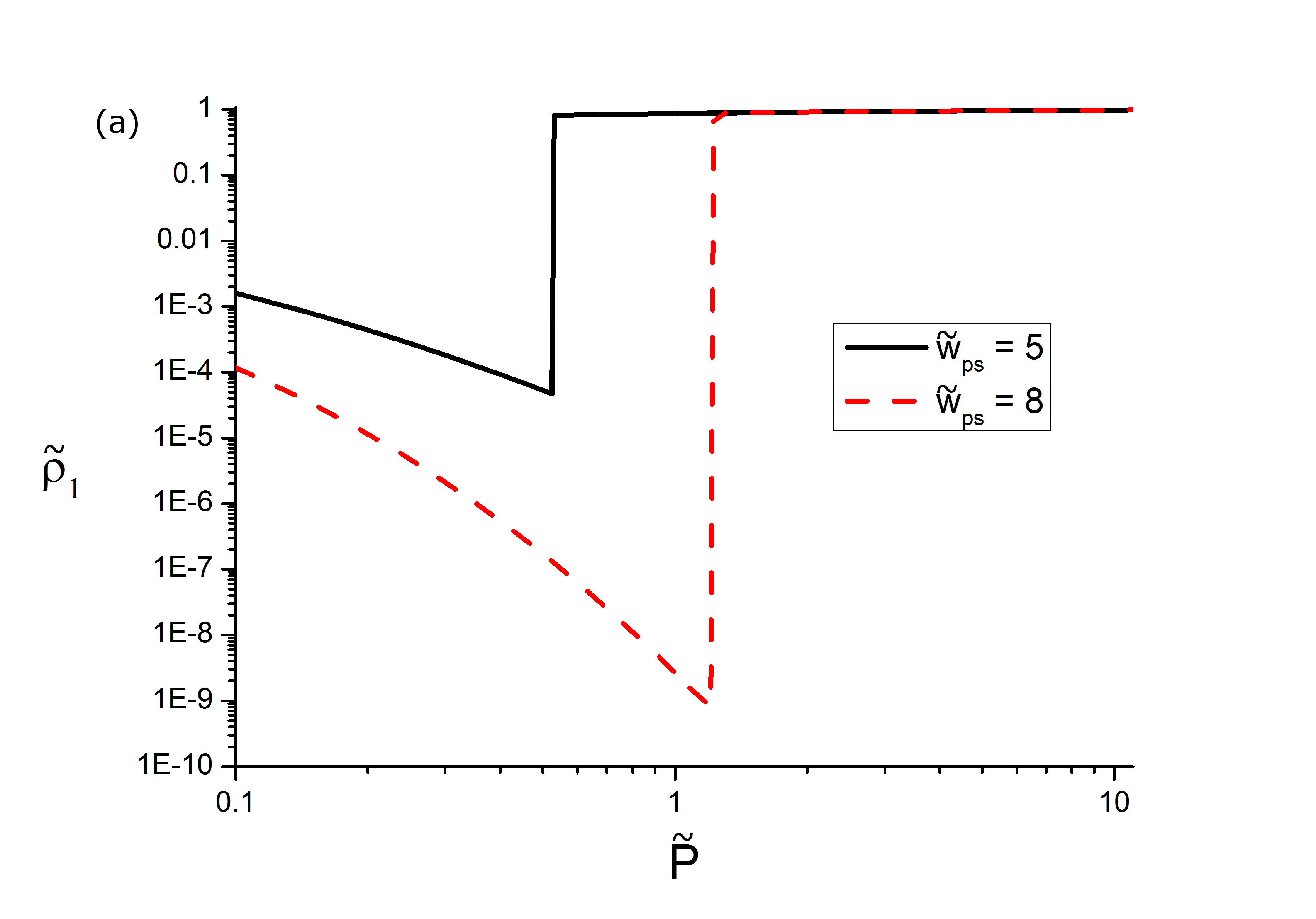
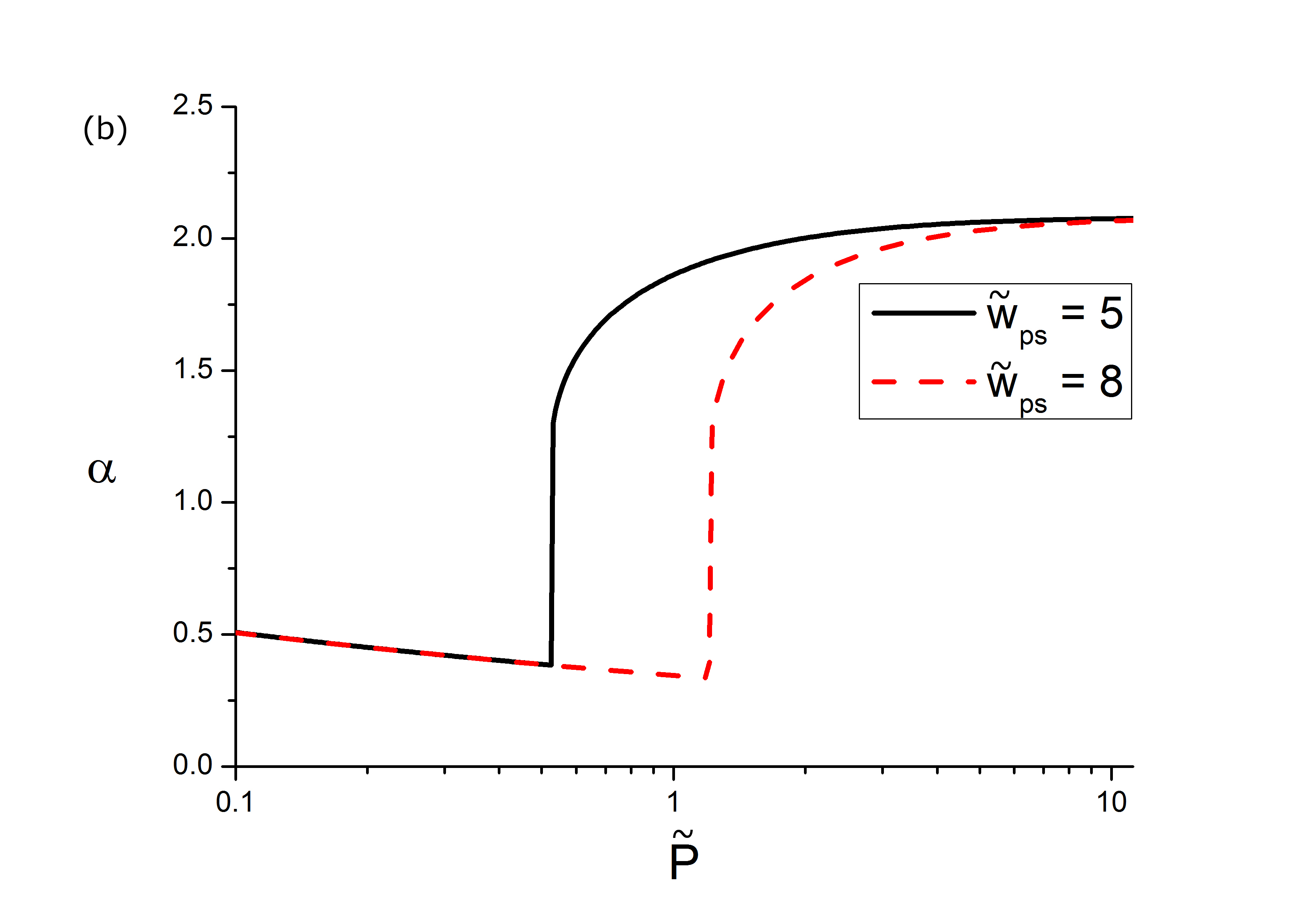
Figure 1: The liquid-phase region of the solvent. (a) The average solvent concentration in the gyration volume $\tilde{\rho}_{1}$ as a function of the solvent pressure in the bulk $\tilde{P}$ shown for two different solvophobic strength $\tilde{w}_{ps}=5;8$. (b) The expansion factor $\alpha$ as a function of the solvent pressure in the bulk solution $\tilde{P}$ shown for the same solvophobic strengths $\tilde{w}_{ps}=5;8$. Values are shown for $\tilde{v}_{s}=1$, $\tilde{w}_{p}=1$, $N=10^{3}$, $\tilde{T}=0.27$.

We first discuss the case when the temperature $\tilde{T}$ of the system is below the critical temperature $\tilde{T}_{c}=\frac{8}{27}$ of the solvent ($\tilde{T}<\tilde{T}_{c}$) for different solvophobic strength $\tilde{w}_{ps}$. Hence, we consider the isotherm $\tilde{P}=\tilde{P}(\tilde{\rho},\tilde{T})$ increasing $\tilde{\rho}$ starting from the binodal. Fig. 1 (a) shows the solvent number density in the gyration volume as a function of the solvent pressure in the bulk at a fixed solvophobic strength $\tilde{w}_{ps}$. Increasing the pressure $\tilde{P}$ in the bulk, the solvent concentration in the gyration volume decreases monotonically and at some threshold value jumps to a value which is very close to the bulk solvent number density. The expansion factor in this range (Fig.1 (b)) abruptly changes the globular regime (36) and then jumps to the regime of the polymer coil (45). The jumps of $\tilde{\rho}_{1}$ and $\alpha$ are a consequence of the penetration of the solvent into the gyration volume leading to the equilibration of pressures between the gyration volume and the bulk solution. This amounts to a gas-liquid transition of the solvent within the gyration volume (Fig. 1 (b)).

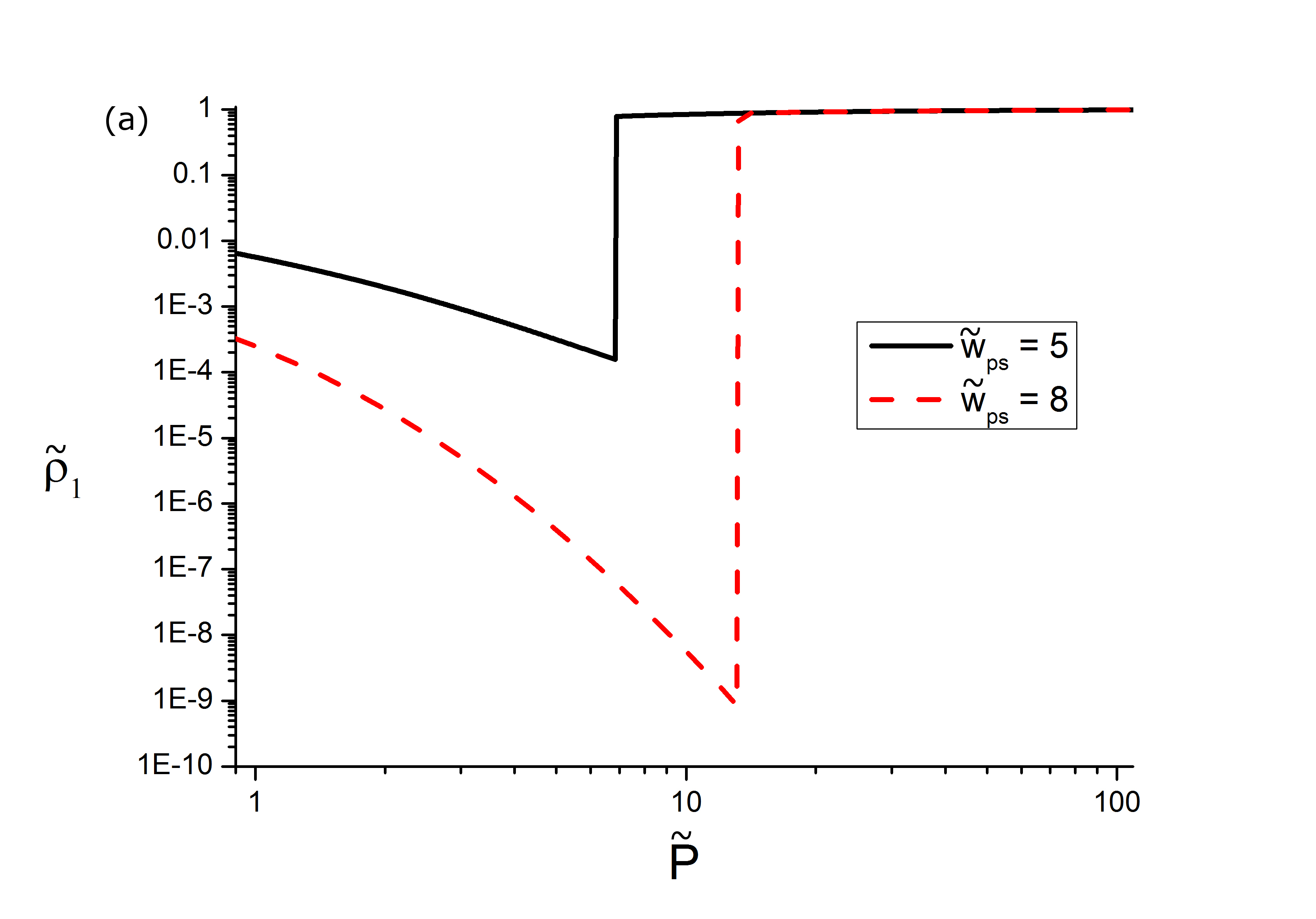
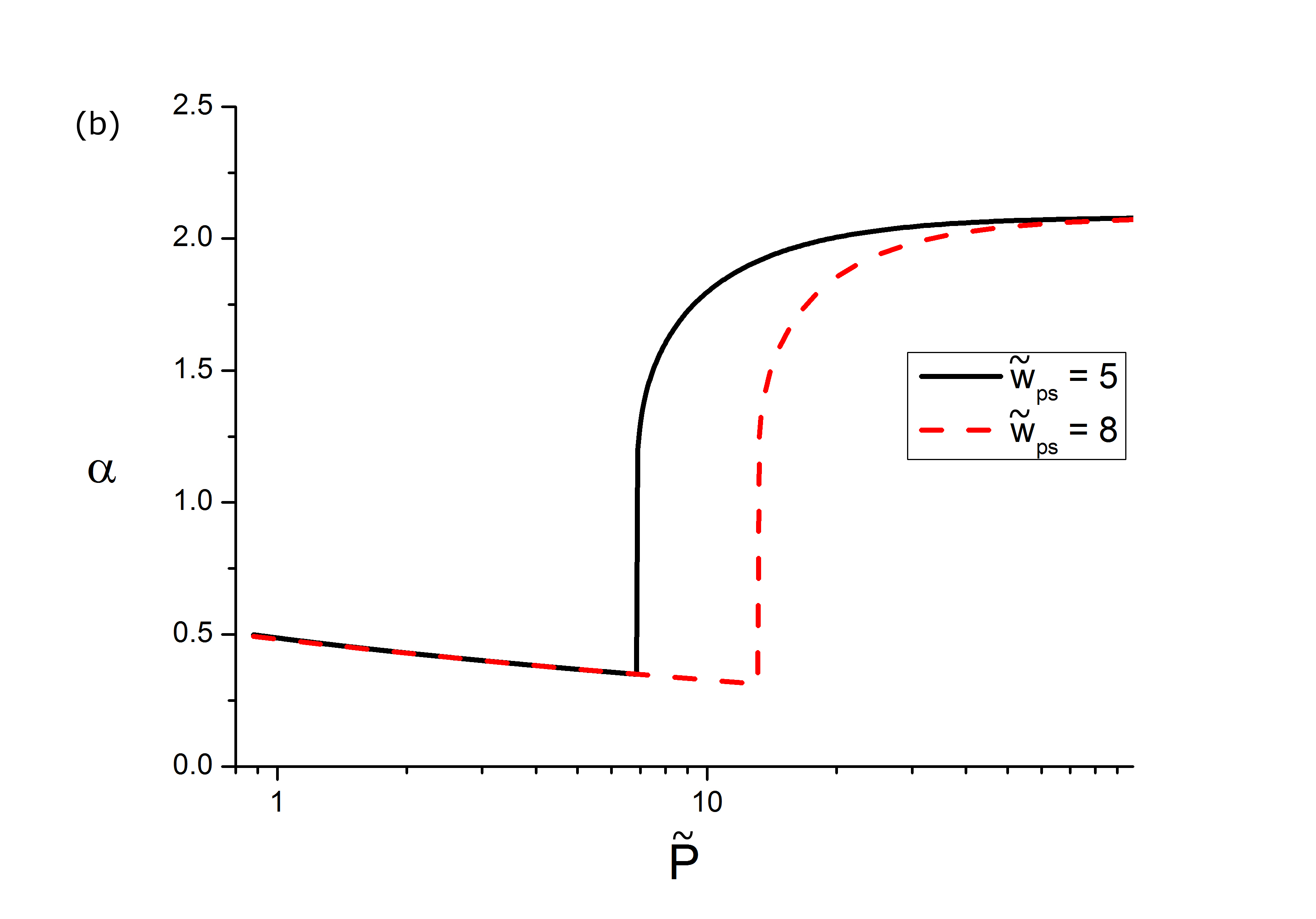
Figure 2: The supercritical region of the solvent ($\tilde{T}>\tilde{T}_{c}$,  $\tilde{\rho}>\tilde{\rho}_{c}$). (a) The average solvent concentration in the gyration volume $\tilde{\rho}_{1}$ as a function of the solvent pressure in the bulk $\tilde{P}$ shown for the solvophobic strength $\tilde{w}_{ps}=5;8$. (b) The expansion factor $\alpha$ as a function of the solvent pressure in the bulk solution $\tilde{P}$ shown for the same solvophobic strength $\tilde{w}_{ps}=5;8$. The behavior of the expansion factor and the average solvent concentration within the gyration volume is quite similar to the behavior in region below critical isotherm ($\tilde{T}<\tilde{T}_{c}$). Values are shown for $\tilde{v}_{s}=1$, $\tilde{w}_{p}=1$, $N=10^{3}$, $\tilde{T}=2$.

Now we turn to the discussion of the region where $\tilde{T}>\tilde{T}_{c}$. We increase the solvent number density from critical one (Fig. 2 (a,b)), so that we consider behavior of polymer chain in the supercritical region of solvent. The results for a polymer chain in the supercritical solvent region ($\tilde{T}>\tilde{T}_{c}$, $\tilde{\rho}>\tilde{\rho}_{c}$), increasing the solvent number density up from critical point are shown in (Fig. 2 (a,b)).

Quite similar behavior occurs in the present case compared to the region where $\tilde{T}<\tilde{T}_{c}$. The presence of jumps in the solvent concentration $\tilde{\rho}_{1}$ and in the expansion factor $\alpha$ are also here due to the effect of the solvent molecules intruding into the gyration volume which in turn leads to an equilibrium between the pressure in the gyration volume and the bulk.

It is instructive to regard the dependence of the expansion factor on the solvophobic strength in the regions below ($\tilde{T}>\tilde{T}_{c}$) and above ($\tilde{T}<\tilde{T}_{c}$) the critical isotherm of the solvent. Fig.3 (a) shows such dependence at fixed bulk solvent concentration. In both cases a polymer chain collapse occurs to the regime (36) when the solvophobic strength exceeds a threshold value. It should be noted, that the polymer chain collapse in region $\tilde{T}>\tilde{T}_{c}$ occurs at higher solvophobic strength than in the region $\tilde{T}<\tilde{T}_{c}$. We would also like to stress that the polymer chain collapse occurs as a first-order phase transition, confirming the hypothesis of ten Wolde and Chandler Chandler_2002 . Indeed, as shown in Fig. 3 (b) the solvent concentration in the gyration volume attains to very small values when the polymer chain collapse takes place. In the region below the solvent critical isotherm this jump corresponds to a dewetting transition which results in a formation of a polymer globule surface surrounded by a layer of solvent gas. In the region above the critical isotherm a similar mechanism is responsible for the transition. However, in this case the collapse is caused by a layer of a gas-like fluid.

It should be noted that at higher degree of polymerization $N$ the globule expansion is more pronounced. The Fig.4 shows the expansion factor $\alpha$ as a function of pressure for different degrees of polymerization $N$. This behavior reflects the well known fact that conformational transitions turn into true phase transitions only in the limit $N\rightarrow\infty$ Moore ; Grosberg_Khohlov .

Finally, we estimate the range of thermodynamic parameters in physical units at which the local solvent evaporation near the polymer chain can occur.

The dimensionless parameters are chosen as in fig.3 (a,b): $\tilde{T}=0.27$ and $\tilde{\rho}=0.7$ (below the critical isotherm). In order to obtain an estimate we choose the parameters as $a_{s}=3.64\leavevmode\nobreak\ L^{2}bar/mol^{2}$ and $v_{s}=0.04\leavevmode\nobreak\ L/mol$ and $a_{s}=5.54\leavevmode\nobreak\ L^{2}bar/mol^{2}$ and $v_{s}=0.03\leavevmode\nobreak\ L/mol$, which correspond to carbon dioxide ($CO_{2}$) and water, respectively WanderVaals_fluid . For $CO_{2}$ we obtain $T\approx 280\leavevmode\nobreak\ K$, $P\approx 280\leavevmode\nobreak\ bar$ and for water $T\approx 590\leavevmode\nobreak\ K$, $P\approx 830\leavevmode\nobreak\ bar$. These estimates show that the discussed local solvent evaporation may be observed under experimentally accessible conditions.

V Summary

Based on a self-consistent field theory taking the solvent explicitly into account, we have described two new effects: a polymer collapse due to the strong polymer-solvent repulsion accompanied by the solvent evaporation within gyration volume and a globule-coil transition at high solvent pressures in the bulk solution accompanied by the solvent condensation near the polymer backbone.

Thus, the theory provides at the mean-field level a quantitative explanation of the dewetting-induced polymer chain collapse, predicted by ten Wolde and Chandler Chandler_2002 .

As a possible extension of the presented theory the solvent concentration fluctuations could be taken into account. This would lead to an additional correction term in the expression of the total free energy which is related to the so-called short-ranged solvent-mediated interactions as described by Fisher and de Gennes Fisher_1978 . Accounting for these non direct fluctuation interactions leads to a renormalization of second virial coefficient of the monomer-monomer interaction Vilgis ; Erukhimovich_JETP ; Budkov_2014 . Such approach has been devised describing the hydrophobic effect at small and large scales by coarse-grained models and incorporating solvent density fluctuations tenWolde_2001 ; Willard_2008 ; Chandler_2011 . The role of the solvent density fluctuations in the vicinity of the critical point in thermodynamics of dilute polymer solutions has been investigated in works Erukhimovich_JETP ; Vilgis within a field theoretical approach. We believe, that such corrections will not change qualitatively our final mean-field results, although it will become significant in the vicinity of the critical point.

Concluding we would like to speculate about possible applications of the presented theory. We believe that our theoretical model could find use when interpreting experimental data on solubility of polymers in supercritical solvents Solubility_1 ; Solubility_2 ; Solubility_3 . Secondly, we believe that the present theory could be used to describe the protein unfolding at high pressures, which has been observed in experiments Winter_1 .

This would, however, require an extension of the theory taking into account hydrogen bond formation between polymer backbone and the solvent molecules, incorporating attractive interaction between a fraction of monomers. Many-body effects arising from long range electrostatic interactions would have to be taken into account as well. Moreover, the refinements of the theory would allow to address the protein folding problem and the structural rearrangements of the protein globule (liquid-solid and solid-solid transitions). However, at the level of the mean-field theory, which does not take into account the effect of short ranged particle correlations, the liquid-liquid and liquid-solid transitions will remain indistinguishable.

Figure 3: (a) The expansion factor $\alpha$ as a function of solvophobic strength $\tilde{w}_{ps}$ at fixed solvent concentration in the bulk ($\tilde{\rho}=0.7$) below and above the critical isotherm of the solvent. (b) The average solvent concentration within the gyration volume $\tilde{\rho}_{1}$ as a function of solvophobic strength $\tilde{w}_{ps}$ at fixed solvent concentration in the bulk ($\tilde{\rho}=0.7$) below and above the critical isotherm of the solvent. In both cases at some threshold value of solvophobic strength the polymer chain collapse occurs. For a polymer chain collapse above the critical isotherm a sufficiently higher solvophobic strength is required than that in region below critical isotherm. Polymer chain collapse occurs as a first-order phase transition. Values are shown for $\tilde{v}_{s}=1$, $\tilde{w}_{p}=1$, $N=10^{3}$.

Figure 4: The expansion factor $\alpha$ as a function of the solvent pressure in the bulk solution $\tilde{P}$ shown for $N=10^{2};10^{3};10^{4}$. At increasing of degree of polymerization the globule-coil transition occurs more dramatically. Values are shown for $\tilde{v}_{s}=1$, $\tilde{w}_{p}=1$, $\tilde{w}_{ps}=5$.

References

- (1) ten Wolde P.R. and Chandler D., PNAS , 10, p. 6539, (2002).
- (2) de Gennes P.-G., Scaling Concepts in Polymer Physics Cornell University Press, 1979.
- (3) A.Yu. Grosberg and A. R. Khokhlov, Statistical Physics of Macromolecules AIP, New York, 1994.
- (4) Edwards S.F., Proc. Phys. Soc. , p. 613, (1965).
- (5) Edwards S.F., Proc. Phys. Soc. , p. 265, (1966).
- (6) Birshtein T.M. and Pryamitsyn V.A., Macromolecules , p. 1554, (1991).
- (7) Birshtein T.M. and Pryamitsyn V.A., Polymer Science U.S.S.R. , 9, p. 2039, (1987).
- (8) Moore M.A., J. Phys. A: Math. Gen. , 2, p. 305, (1977).
- (9) Lifshitz I.M. and Grosberg A.Yu, Soviet physics JETP. - , 6, p. 1198, (1974).
- (10) Lifshitz I.M., Soviet physics JETP , 6, p. L-55, (1975).
- (11) de Gennes P.G., Le Journal De Physique - Letters , 2, p. 55 (1975).
- (12) Muthukumar M., J. Chem. Phys. , p. 6272, (1984).
- (13) Sanchez I.C., Macromolecules. , 5, p. 980, (1979).
- (14) Kholodenko A.L. and Freed K.F., J. Phys. A: Math. Gen. , p. 2703, (1984).
- (15) Grosberg A.Yu. and Kuznetsov D.V., Macromolecules , p. 1970, (1992).
- (16) Grosberg A.Yu. and Kuznetsov D.V., Macromolecules , p. 1980, (1992).
- (17) Grosberg A.Yu. and Kuznetsov D.V., Macromolecules , p. 1991, (1992).
- (18) Grosberg A.Yu. and Kuznetsov D.V., Macromolecules , p. 1996, (1992).
- (19) Khohlov A.R., Physica , p. 357, (1981).
- (20) J. M. P. van den Oever, F. A. M. Leermakers, G. J. Fleer, V. A. Ivanov, N. P. Shusharina, A. R. Khokhlov, and P. G. Khalatur, Phys. Rev. E. , p. 041708, (2002).
- (21) Schultz R.C. and Flory P., J. Polym. Sci. , p. 231, (1955).
- (22) Brochard F. and de Gennes P. G., Ferroelectrics. , p. L-59, (1980).
- (23) Vilgis T., Sans A., and Jannink G., J. Phys. II France , p. 1779, (1993).
- (24) Dua A. and Vilgis T.A., Macromolecules, , p. 6765, (2007).
- (25) Dua A. and Cherayil B.J., J. Chem. Phys. , 7, p. 3274, (1999).
- (26) Lifshitz I.M., Grosberg A.Yu., A.R. Khohlov, Rev. Mod. Phys. , 3, p. 683, (1978).
- (27) Erukhimovich I.Ya., Journal of Experimental and Theoretical Physics , 3, p. 494, (1998).
- (28) Matsuyama M. and Tanaka F., J. Chem. Phys., , 1, p. 781, (1991).
- (29) Tanaka F., Koga T. and Winnik F.M., Phys. Rev. Lett., , p. 028302, (2008).
- (30) Budkov Yu.A., Kolesnikov A.L., Georgi N., and Kiselev M.G., J. Chem. Phys. , p. 014902, (2014).
- (31) Fredrickson G. H. The Equilibrium Theory of Inhomogeneous Polymers Oxford: Clarendon Press, 2006.
- (32) Fixman M., J. Chem. Phys. , 2, p. 306, (1962).
- (33) Flory P., Statistical Mechanics of Chain Molecules New York: Wiley-Interscience, 1969.
- (34) Barrat J.-L. and Hansen J.-P. Basic Concepts for Simple and Complex Liquids University Press, Cambridge, 2003.
- (35) ten Wolde P.R., Sun S.X., and Chandler D., Phys. Rev. E. , p. 011201, (2001).
- (36) Willard A.P. and Chandler D., J. Phys. Chem. B , p. 6187, (2008).
- (37) Varilly P., Patel A.J., and Chandler D., J. Chem. Phys. , p. 074109, (2011).
- (38) Fisher, M. E. and de Gennes, P. G., C. R. Acad. Sci. Paris B. , p. 207, (1978).
- (39) Weast R. C. Handbook of Chemistry and Physics Cleveland: Chemical Rubber Co., 1972.
- (40) Dardin A., Cain J.B., DeSimone J.M., Johnson, Jr C.S., Samulski E.T. , Macromolecules , 12, p. 3593, (1997).
- (41) Andre P., Lacroix-Desmazes P., Taylor D.K., and Boutevin B., J. of Supercritical Fluids , p. 263, (2006).
- (42) Kiran E., J. of Supercritical Fluids , p. 466, (2009).
- (43) Herberhold H. and Winter R. // Biochemistry , p. 2396, (2002).
- (44) Kubo R., J. Phys. Soc. Jap. , p. 1100, (1962).
- (45) Tamm M.V., Erukhimovich I.Ya., Polymer Science, Ser. A, , 2, p. 196, (2002).