Large Magnetic Shielding Factor Measured by Nonlinear Magneto-optical Rotation

Abstract

A passive magnetic shield was designed and constructed for magnetometer tests for the future neutron electric dipole moment experiment at TRIUMF. The axial shielding factor of the magnetic shield was measured using a magnetometer based on non-linear magneto-optical rotation of the plane of polarized laser light upon passage through a paraffin-coated vapour cell containing natural Rb at room temperature. The laser was tuned to the Rb D1 line, near the ⁸⁵Rb $F=2\rightarrow 2,3$ transition. The shielding factor was measured by applying an axial field externally and measuring the magnetic field internally using the magnetometer. The axial shielding factor was determined to be $(1.3\pm 0.1)\times 10^{7}$, from an applied axial field of 1.45 $\mu$T in the background of Earth’s magnetic field.

1 Introduction

The next generation of neutron electric dipole moment (EDM) experiments aim to measure the EDM $d_{n}$ with proposed precision $\delta d_{n}\lesssim 10^{-27}$ e-cm [1, 2, 3, 4, 5, 6, 7, 8, 9]. In the previous best experiment [10], which discovered $d_{n}<2.9\times 10^{-26}$ e-cm, effects related to magnetic field homogeneity and instability were found to dominate the systematic error. A detailed understanding of passive and active magnetic shielding, magnetic field generation within shielded volumes, and precision magnetometry is expected to be crucial to achieve the systematic error goals for the next generation of experiments. Much of the R&D effort for these experiments is focused on careful design and testing of various magnetic shield geometries with precision magnetometers [11, 12, 13, 14, 15].

Our work focused on the creation of a new small-scale magnetic shield designed primarily for magnetometer tests for our future nEDM experiment at TRIUMF. Within the shield, we prepared a magnetometer based on non-linear magneto-optical rotation (NMOR). NMOR results in a rotation of the plane of polarization of laser light resonant with atomic transitions in Rb vapour. In NMOR, the optical properties of the medium are modified by the laser light, resulting in nonlinear effects such as hole-burning and the creation of a coherent dark state [16]. The combined effect results in ultranarrow linewidths of $\sim$Hz, corresponding to projected field sensitivities at the few fT level [17]. The effect, which occurs near zero field, can be displaced to a non-zero field using either a frequency-modulated (FM) [18] or amplitude-modulated (AM) [19, 20, 21] pump beam, and a CW probe beam, and can in principle retain $\sim$fT precision [22]. At such precision, the technology is superior to fluxgate magnetometers, and rivals the precision of SQUID magnetometers, without the need for cryogenics. Recently, a three-axis NMOR-based magnetometer has been demonstrated [15].

Our magnetometer was based on the zero-field effect along a single axis. By calibrating the zero-field magnetometer using coils internal to the magnetic shield, we determined the axial magnetic shielding factor for fields applied by external coils. A key result of this work is that very large DC shielding factors could be measured in a small space, for small applied external fields (more than an order of magnitude smaller than Earth’s field). Such measurements could not have been conducted using a conventional fluxgate magnetometer. The results validate our initial design goals for the magnetic shielding. The results also highlight the applicability of precision NMOR-based magnetometers in magnetically shielded environments, such as those that will be seen in future neutron EDM experiments.

2 Passive Magnetic Shield System

Analytical approximations exist for the transverse and axial shielding factors of completely closed and open finite multi-layered cylindrical shapes made of a high permeability $\mu$ material [23, 24, 25, 26]. Here transverse (axial) shielding implies a reduction in the externally applied magnetic field that is perpendicular (parallel) to the axis of concentric cylindrical shells. Closed-ended cylindrical structures have a higher axial shielding factor than open-ended concentric shells [23]. Shield structures often need apertures permitting access to the internal shielded volume for e.g. laser light, subatomic particles, wires for field generation, etc. Often cylindrical extensions, or “stovepipes”, are situated around the apertures. Stovepipes generally may increase the shielding factor, however the optimum length is highly dependent on the design constraints and parameters of the shield structure. The shield used in this work was designed using a commercial finite element analysis (FEA) software package [27]. Special care was taken to design the apertures and stovepipes in the ends of the shield achieving as large as possible axial magnetic shielding factor.

2.1 Design Constraints

The shield was designed in using FEA by requiring that the magnetic field within a region of interest (ROI) internal to the shield be as small as possible under application of an external axial field. For design purposes, the ROI was selected to be 4” (10.16 cm) long and 1” (2.54 cm) diameter, corresponding to the space inhabited by most magnetometers of interest. The innermost shield was required to be at least 4” (10.16 cm) in diameter and 8” (20.32 cm) long, in order to accommodate various coils as well as the magnetometers and support structures. The outermost shield diameter was required to be less than 12” (30.48 cm) to keep the shield small enough to rest on an optics table. All access to the inner shield was to be provided by a single $1\frac{1}{8}$” (2.86 cm) protrusion on each end to admit laser light along the axis (as well as cabling for field coils). Only the axial shielding factor was considered in designing the shield, because the axial shielding factor is generally smaller than the transverse shielding factor for this geometry.

The material to be used for the shield was fixed at 1/16” (0.159 cm) thick, since this material is readily available and cost effective. Both three- and four-layer shields were considered. Initial estimates of the axial shielding factor were conducted by comparing the results of the approximate axial shielding factors of Refs. [23]. A stovepipe geometry on the axial 2.86 cm protrusion in each shield layer was considered based on the analytical result found in Ref. [31] for the exponential decay of an axial field leaking into an open-ended cylinder.

A starting design based on these considerations was then implemented in the FEA simulation. The length $L_{i}$ and radius $R_{i}$ of each shielding layer $i$, the number of layers ($N=3$ or $4$ where $1\leq i\leq N$ and $i=1$ refers to the innermost shield), and the length of the stovepipe $\ell$ were allowed to vary in the simulation. The radii of the shields were constrained to obey $R_{i+1}/R_{i}=c$ where $c$ is a constant independent of the layer. The length of each successive layer was constrained to follow $L_{i+1}=L_{i}+2\ell+R_{i+1}-R_{i}$. Thus there is a gap between the end of a stovepipe and the next layer’s lid of $\frac{1}{2}(R_{i+1}-R_{i})$. This ensures sufficient space between the stovepipes and lids of each layer, i.e. the stovepipes are not nested. Other fractions of this gap were not considered. As expected based on simple estimation, the best results for the shielding factor were found for the larger number of shield layers $N=4$ and the value of $c$ being as large as possible $c=(R_{4}/R_{1})^{1/3}=1.4$ so that $R_{4}=6$” if $R_{1}$ is constrained to be 2”.

A somewhat surprising result was that shorter shields with shorter stovepipes were preferable, in that the additional length implied by longer stovepipes ultimately served only to make the shield longer, with a somewhat negative impact on the overall shielding factor. The FEA result is displayed graphically in Fig. 1. This was found to be qualitatively in agreement with recent work in Ref. [32].

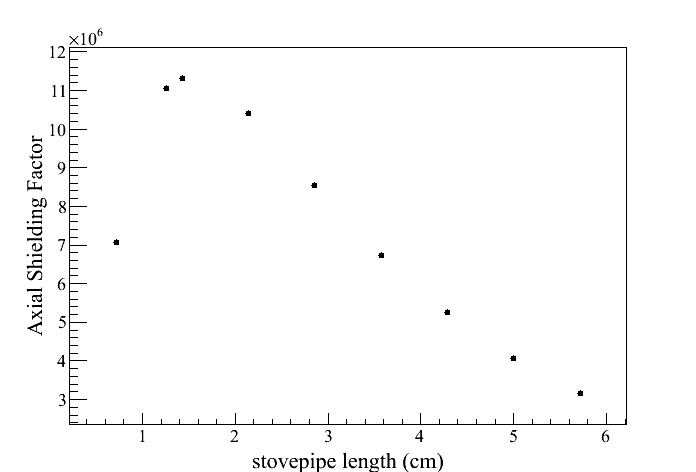
Figure 1: FEA study of axial shielding factor vs. stovepipe length $\ell$ for a four-layer shield with radial dimension as in Fig. 2. Each stovepipe of the next shield was required to be fully contained within the next shield. Under these conditions, the axial shielding factor decreases as the stovepipe length (and therefore overall shield length) increases. The optimal stovepipe length is of order half the hole diameter.

Magnetic field homogeneity using a simple solenoidal internal coil design (reminiscent of the one described in Section 2.3) was also checked in the ROI, and confirmed that the 20.32 cm length of the innermost shield would be sufficient for sub-percent homogeneity over the ROI.

2.2 Final Design and Fabrication

The final design is shown in Fig. 2 and the dimensions as constructed were similar. The magnetic shield was fabricated and annealed by Ad-Vance Magnetics, Inc. [28]. The vendor informally suggested an effective DC permeability relative to that of free space $\mu_{r}=20,000$ for the AD-MU-80 material used for the shield. Using this value in our FEA simulations implied an anticipated axial magnetic shielding factor of $1.1\times 10^{7}$.

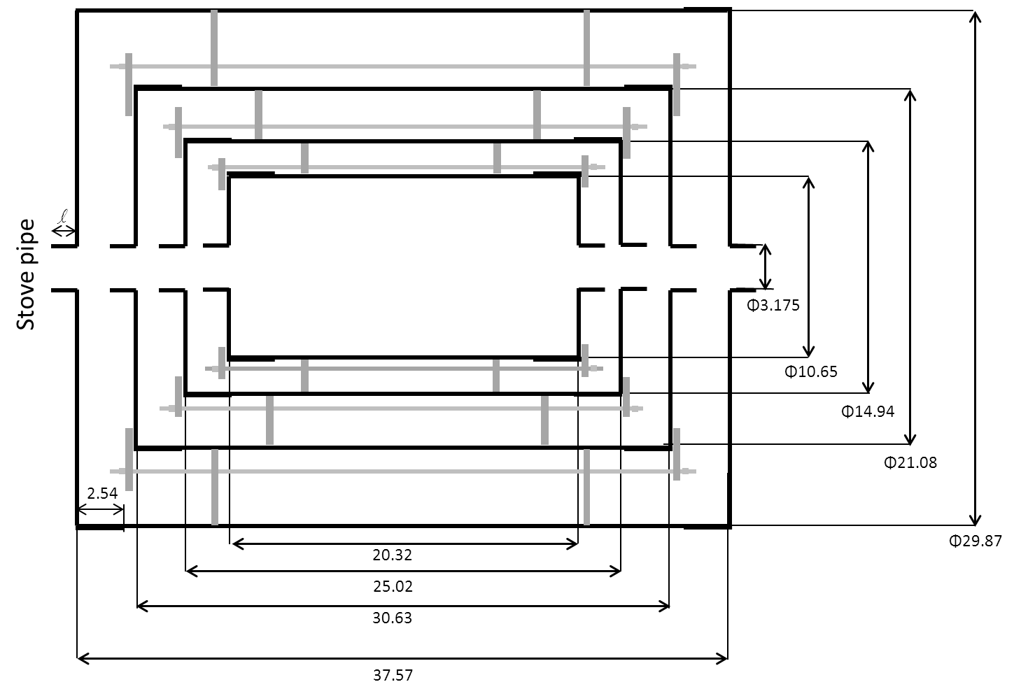
Figure 2: Schematic diagram of the 4-layer magnetic shield (dimensions in cm). Outer diameters of the cylinders are shown, and dimensions are quoted in centimeters. The diameter of each endcap is larger by 0.1 cm to fit over its corresponding cylinder, extending 2.54 cm over the end of it. The hole diameter and stovepipe length for each endcap are the same. High density polyethylene spacers and nylon thread rods/nuts, shown in gray, hold the shields and end caps together.

2.3 Internal Coils

An internal coil, henceforth referred to as the $z$-coil, provided a uniform field in the ROI, directed along the axis of the cylindrical volume. The $z$-coil was wound on a 7.62 cm diameter, 20.32 cm long ABS plastic pipe. Seven turns of 26 AWG magnet wire were wound at 2.54 cm spacing, with 1.27 cm spacing from the magnetic faces of the endcaps of the innermost magnetic shield. The spacings were chosen so that, in the infinite permeability limit, and in the limit where the axial aperture holes in the endcaps are small, the boundary conditions would produce image currents forming an infinitely long solenoid [29, 30]. This is similar to the design strategy used in Ref. [16]. Two saddle coils were wound on the same cylinder in order to control transverse fields internally; these were normally disconnected during precision measurements.

The internal coil system was calibrated using a three-axis fluxgate magnetometer at fields of $\sim$100 nT. The calibration of the $z$-coil was verified using the NMOR magnetometer with an AM pump beam, and the known gyromagnetic ratios of Rb-85 and Rb-87 (described in Section 3 and similar to Ref. [20]).

Homogeneity of the residual field and magnetic field generated by the coil system was measured by scanning a fluxgate magnetometer along the axis of the system with and without the coil energized. At a field of 1 $\mu$T, the axial field generated by the coil was uniform within the ROI to the 1% level.

A single degaussing coil formed from a single loop of 12 AWG multi-stranded insulated copper wire was fed through all four endcaps and wound tight to both the innermost shield surface and outermost shield surface. In degaussing, a Variac was used to slowly ramp the current in the degaussing coil, by hand, from zero to 10 A and down again. A 100 $\Omega$ power resistor in series with the degaussing coil was used to limit the current the Variac delivered. The system provided zero magnetic field within the system reliably to the $<0.3$ nT level. Multiple degaussing trials would reduce this to the $<0.1$ nT level, which was sufficient for the measurements conducted using the NMOR-based magnetometer. During precision magnetometer measurements, the degaussing coil would be disconnected from its power supply.

3 NMOR magnetometer

A schematic diagram of the NMOR magnetometer system is shown in Fig. 3. Laser light was provided by a Toptica DL-100 external cavity diode laser [33], tuned to the Rb D1 line. Light impinged upon a vapour cell containing natural Rb, placed at the center of the coil and shield system.

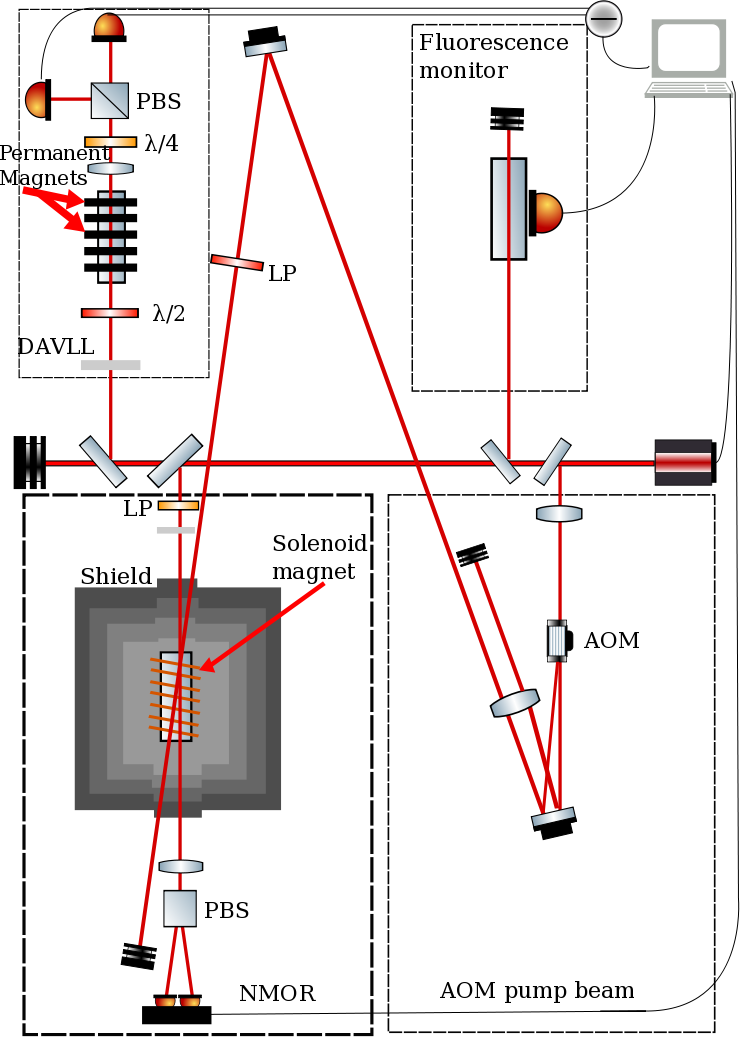
Figure 3: Schematic diagram (top view) of magnetic shield and NMOR magnetometer system. The main NMOR experiment is conducted by splitting off a fraction of the beam from the laser into the magnetic shield system and through the Rb vapour cell within. Optical rotation is measured using a polarizing beam splitter (PBS, being a Wollaston prism) followed by a balanced photosensor. For the results in this publication, this beam served as both pump and probe. An acousto-optic modulator (AOM) may be used to provide an amplitude-modulated pump beam, using the previously mentioned system as a probe, thereby creating a magnetometer capable of measuring fields far from $B=0$ (similar to Ref. [20]); for this work, the pump beam was used only during a calibration cross-check on the magnetic field generated by the internal coil. The fluorescence monitor is used in beam tuning and the DAVLL system is used to lock the laser frequency.

The vapour cell was cylindrical, 5 cm long and 5 cm in diameter with optical flats on the ends. The cell was provided by D. Budker, having been prepared in a fashion similar to the cells described in Ref. [34]. The cell was characterized using a method similar to Ref. [34], by measuring the relaxation of longitudinal polarization using optical rotation as a probe. The long time component of the relaxation was thereby found to decay with a time scale of 0.36 s.

The temperature of the vapour cell was controlled by the ambient temperature of the surrounding room ($\sim 21^{\circ}$C). Transmitted light was analyzed for optical rotation by a balanced polarimeter system containing a Wollaston prism and a Newport model 2307 balanced photoreceiver [35].

The power delivered to the vapour cell was typically 15 $\mu$W, measured periodically using a Newport Model 818-SL power meter [35] inserted into the beamline. The laser was first tuned near the Rb-85 $F=2$ to $F^{\prime}=2,3$ absorption minimum (fluorescence maximum), then further tuned to maximize optical rotation for $\sim 100$ pT applied fields. The laser frequency was stabilized using a dichroic atomic vapour laser lock (DAVLL) system [36] containing optics for additional locking flexibility based on Ref. [37], and using the Toptica DigiLock 110 system [33].

After degaussing the magnetic shield system, and tuning and locking the laser, the optical rotation as a function of field applied by the internal coil system was measured; the results are displayed in Fig. 4. The amplitude of the optical rotation was $\pm 9$ mrad. The width of the NMOR feature was characterized by fitting the data to the derivative of a Lorentzian. The valley-to-peak field separation was thereby determined to be 400 pT. The results are similar to previous work by others [17].

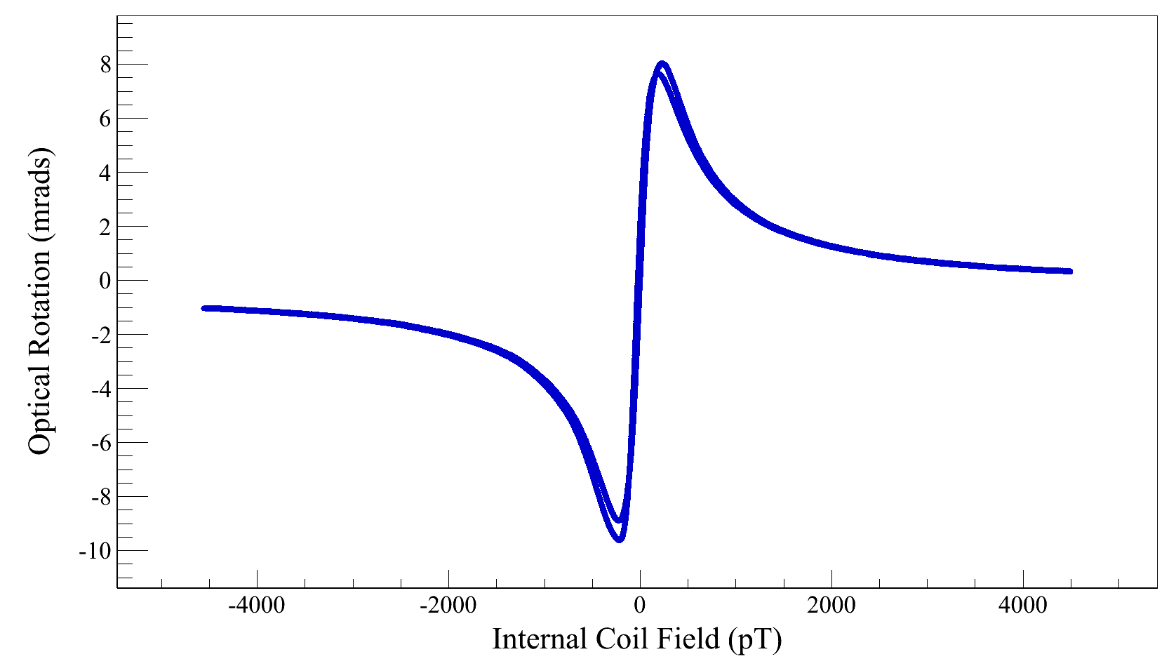
Figure 4: Optical rotation as a function of magnetic field applied along the direction of the laser beam. Data were acquired by sweeping the magnetic field in a triangle wave with a period of 100 s; the peaks in the curve show a slight dependence on the direction of the sweep, due to the time response of the atoms.

The definition of zero optical rotation was not carefully controlled in these measurements; it was adjusted periodically to ensure the signal from the balanced photoreceiver was near zero. The vertical scale of Fig. 4 therefore contains a small arbitrary offset. The horizontal positioning of the zero-field point in the graph refers to zero current applied by the internal solenoidal coil. This is displaced by 15 pT from the steepest point of the NMOR data because of the remanent magnetization of the magnetic shield system, which we did our best to remove via degaussing.

The dispersive feature in Fig. 4 could be narrowed somewhat by applying constant fields with the internal saddle coils (described in Sec. 2.3) as the $z$-coil was swept through zero field. The narrowest spectrum was found by applying an internal transverse field of 130 pT, implying that after degaussing, a residual transverse field of order this magnitude remained. For the measurements presented in this paper, the transverse coils were switched off and disconnected from their power supply in order to avoid additional sources of noise. The method of calibrating optical rotation to the current in the internal $z$-coil makes our method insensitive to static transverse fields, excepting that the magnetometer sensitivity is reduced slightly in a non-zero transverse field. The calibration and method is described in Section 4.

We found we were able to better degauss our shields by determining the remanent longitudinal and transverse fields by requiring graphs like Fig. 4 cross zero as close as possible to zero applied current, and be as narrow as possible for zero applied transverse field. The status of the shields for this measurement represents our best efforts to use the degaussing system in this fashion.

The bandwidth of the magnetometer was measured by applying a sinusoidal magnetic field using the internal $z$-coil, of amplitude 0.5 pT, and measuring the amplitude of optical rotation, which varied sinusoidally at the same frequency. The amplitude of the optical rotation signal was found to drop to $1/\sqrt{2}$ its value at low frequencies for an applied frequency of 2.7 Hz, indicating the -3 dB point of the magnetometer.

Noise in the magnetometer was characterized by measuring the linear spectral density, with the internal coils switched off and disconnected. A graph of the linear spectral density is shown in Fig. 5. The noise was found to be 30 fT/$\sqrt{\rm Hz}$ at a frequency of 1 Hz. A roll-off in noise is seen above 2.5 Hz, as expected, since the sensitivity of the magnetometer is reduced above these frequencies. A peak is seen for frequencies $<0.4$ Hz due to uncorrected DC offsets.

Figure 5: Linear spectral density of noise in the magnetometer when all coils systems are disconnected. The window function HFT116D was used, with the overlap recommended in Ref. [38].

The noise of the magnetometer was also estimated by observing the optical rotation for very small fields applied in a square-wave using the internal $z$-coil, with the bandwidth of the balanced polarimeter limited to 1 Hz using a Stanford Research Systems low-noise preamplifier (Model SR560) [39]. The smallest change in the DC field that could be observed reliably was of order 40 fT under these conditions, consistent with the determination based on the spectral density.

4 Axial shielding factor measurement using very small applied field

An external axial magnetic field was applied to the shield using two circular coils of diameter 30 cm and spaced by 45 cm. Each coil was formed from a single loop of 24 AWG wire. The coils were spaced symmetrically from the endcaps of the magnetic shield. The axial field generated at the center of the coils in the absence of the shield was measured to be 1.45 $\mu$T/A with a fluxgate magnetometer, in agreement with expectation.

In order to measure the axial shielding factor, the internal $z$-coil and the external coil were operated by different square-wave function generators and the optical rotation was observed as a function of time. The internal coil was set to provide a field of $\pm 480$ fT with a period of 20 s. The external coil was set to provide a current of $\pm 1$ A (resulting in a central field $B_{c}=\pm 1.45\mu$T in the absence of the shield) with a period of 4 s. Fig. 6 displays the optical rotation measured as a function of time during this measurement. Since the internal $z$-coil calibration is known, this data enables a determination of the axial field produced internally by the external coils, under the assumption that optical rotation is linear in the axial magnetic field (an assumption that was confirmed by calibrating using different internal $z$-coil currents).

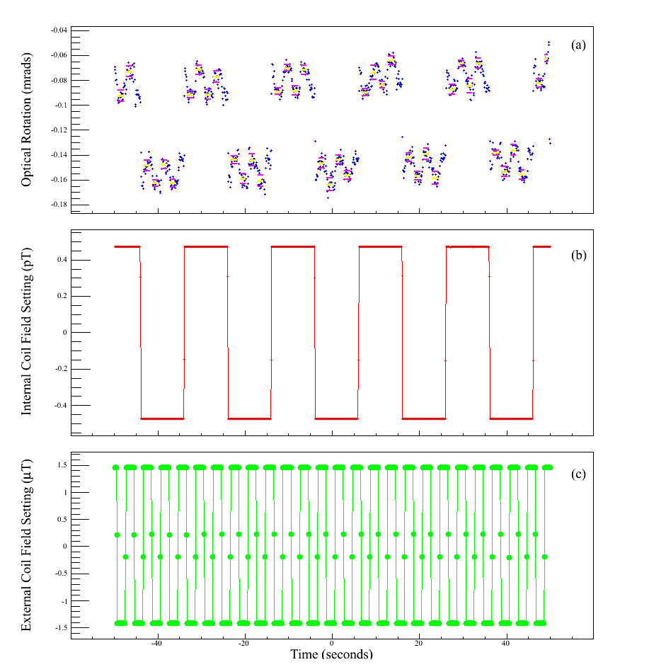
Figure 6: (a) Optical rotation, (b) field generated by the internal $z$ coil, and (c) field generated by the external coil, as a function of time. The optical rotation is seen to depend on both applied fields. Since the field generated by the internal coil is known, the shielding factor for the external field may be determined.

The optical rotation for each setting of the internal and external field in Fig. 6 was averaged. Data within 0.5 s of a transition in the external field were excluded. Data within the 2 s stable period of the external field, but containing a transition in the internal field, were excluded entirely. Typically fourteen optical rotation data points were averaged in each stable period. The result of the averaging was sensitive to changes in these time cutoffs at the $<10\%$ level. The standard deviation for each time period was also determined, and found to be typically 0.005 mrad. In determining the measured fields, successive pairs of measurements were considered in order to eliminate the effect of long-term drifts. The field generated internally by the external coils was thereby determined to be $\pm 110$ fT, or a span of 220 fT.

4.1 Errors in the Measurement

The statistical uncertainty in the measurement comparing successive time-periods in the data is estimated from the standard deviation divided by the square-root of the number of measurements in each period to be 10%. Fifty time periods in the data were averaged, representing twenty-five statistically independent pairs, and the statistical error on the change in internal field is 2% if all time periods are used.

Measurements of optical rotation were occasionally seen to drift over the typical 100 s measurement cycle. In some runs, the drift over 100 s was found to be as large as 0.04 mrad. The source of the drift is unclear at this time, whether a true magnetic change in the shield system (corresponding to a change of $\sim$0.6 pT over the same time period) or a drift in the magnetometer itself. From data taken with all coils disconnected, when drifts occur, the Allan standard deviation is seen to rise for timescales above 1 s. This implies that drifts start to dominate the error for timescales longer than seconds. Taking the 2 s averaging time that we used, with a worst-case drift of 0.04 mrad/100 s the error due to drift within the averaging time would be 5%.

Based on this analysis, considering statistics, drifts, and dependence on time cuts used in the data, the error in the 220 fT internally induced field change from the external coils is $10\%$ or 20 fT.

We defined the axial shielding factor as the reduction of the central $B_{c}=\pm 1.45~{}\mu$T produced by the external coils in the absence of the magnetic shield system to the central field produced at the same position in the presence of the shield. This would agree well with an average over the vapour cell volume (to better than 1%), since the cell dimensions are smaller than the nearest magnetic elements in the system. The shielding factor is then determined from the ratio ($2.9~{}\mu$T)/(220 fT)=$1.3\times 10^{7}$.

4.2 Additional Systematic Studies

The linearity of optical rotation with axial magnetic field was tested by varying the amplitude of the internal $z$-coil field between 200 and 1000 fT; the optical rotation was found to be linear to within the precision of the measurement of the internal field. The optical rotation measured by the balanced polarimeter was calibrated to a physical rotation of a half-wave plate placed in the path of the laser and found to be in agreement with expectation.

The field generated by the external coil in our experiment is not uniform; a larger external coil system was not possible in our setup, because of physical constraints and nearby magnetic elements. A concern in the measurement was that the shield experiences an effectively larger field than the central field of the external coil system would indicate, because of the closeness of the coils to the outermost shield. To test this, the spacing between the coils was increased, thereby increasing the distance of the coils from the outermost shield.

Configuration	Spacing (cm)	Current (A)	$B_{c}$ ($\mu$T)	SF ($\times 10^{6}$)
1	45	$\pm 1.0$	$\pm 1.45$	$13.1\pm 1.3$
2	50	$\pm 1.0$	$\pm 1.15$	$13.8\pm 1.8$
3	60	$\pm 1.0$	$\pm 0.75$	$14.7\pm 3.2$
4	60	$\pm 2.0$	$\pm 1.50$	$13.3\pm 1.3$

Table 1: Shielding factor (SF) for the various configurations of $z$-coil spacing and current. The nominal central field $B_{c}$ in the absence of the shield was determined numerically and verified by fluxgate measurement to within 5%. The uncertainty of 20 fT on the measurement of the internal field via NMOR dominates the error in SF.

Table 1 displays the resultant shield factor determined for various trials where the spacing of the external coils and the current flowing through the external coils was changed. For changes to the geometry of the coil admitted by the physical space limitations of our experiment (corresponding to coil spacings ranging from 45 to 60 cm), the shielding factor was found to vary by 8%, within the stated errors on the measurements. Since the measurements are all in agreement, we retain the result for the shielding factor $(1.3\pm 0.1)\times 10^{7}$.

4.3 Earth’s field, other transverse fields, and limitations

The magnetic shield and coil system were always subject externally to Earth’s magnetic field, which is considerably stronger than the $\pm 1.45\mu$T field supplied by the external coil system. The Earth’s field was dominantly transverse to the axis of the laser beam and shield. In a model where the magnetic material in the shield is linear, the presence of a transverse field of this sort does not affect the axial shielding factor measured using our technique. However, if the material is not linear, the results could depend on the saturation of the material. Our magnetic shielding factor measurements therefore possess this caveat.

Finally, it is possible that the application of an external field by our coil system could generate internal fields that are not entirely longitudinal when averaged over the volume of the vapour cell. This could occur due to any lack of cylindrical symmetry in the system, resulting from e.g. misalignment and imperfections in the magnetic shielding. Furthermore the magnetometer, and our calibration scheme, are sensitive to transverse fields. We measured this sensitivity by applying similar magnitude ($\pm 250$ fT) transverse fields using the internal saddle coils and found the optical rotation to be, at largest, a factor of two smaller for the same field applied axially, and dependent on the direction of the transverse field. Thus, while the sensitivity was smaller, it was not significantly smaller. It is therefore an assumption of the procedure that only the axial field changed when exciting the external coil.

5 Conclusion

We have employed an NMOR-based magnetometer to make measurements of small axial magnetic fields generated within a cylindrical magnetically shielded volume by a pair of external circular coils. The shielding factor for an axially-directed 1.45 $\mu$T field was determined to be $(1.3\pm 0.1)\times 10^{7}$, in the background of Earth’s field. The result was consistent for even lower applied fields of 0.75 $\mu$T. The results reproduce the design expectations of the magnetic shield, which were based on finite element analysis. The results therefore provide a useful benchmark for future magnetic shield design.

The results highlight the applicability of NMOR-based magnetometers for small fields inside magnetically shielded volumes, such as those that will be experienced in future neutron electric dipole moment experiments. In the future we plan to study the stability of NMOR-based magnetometers and the stability of uniform magnetic fields generated by coils internal to the measurement volume, similar to the situation in future EDM experiments.

6 Acknowledgements

We would like to thank D. Budker and B. Patton for their advice on the development of the magnetometer, and for the loan of their vapour cell. This work was supported by the Canada Foundation for Innovation, the Natural Sciences and Engineering Research Council Canada, and by the Canada Research Chairs program.

References

References

- [1] S. N. Balashov et al., arXiv:0709.2428.
- [2] A. P. Serebrov et al., JETP Lett. 99, 4 (2014).
- [3] A. P. Serebrov et al., Physics Procedia 17, 251 (2011).
- [4] K. Kirch, AIP Conf. Proc., Vol. 1560, pp. 90-94 (2013).
- [5] C. A. Baker, et al., Physics Procedia 17, 159 (2011).
- [6] Y. Masuda, K. Asahi, K. Hatanaka, S.-C. Jeong, S. Kawasaki, R. Matsumiya, K. Matsuta, M. Mihara, and Y. Watanabe, Phys. Lett. A 376, 1347 (2012).
- [7] I. Altarev, et al., Nuovo Cim. C 35, 122 (2012).
- [8] R. Golub and S. K. Lamoreaux, Phys. Rept. 237, 1 (1994).
- [9] T. M. Ito (the nEDM collaboration), J. Phys. Conf. Ser. 69 012037, 2007.
- [10] C. A. Baker, et al., Phys. Rev. Lett. 97, 131801 (2006).
- [11] T. Bryś, et al., Nucl. Instrum. Meth. A 554, 527 (2005).
- [12] S. Afach, et al., J. Appl. Phys. 116, 084510 (2014).
- [13] I. Altarev, et al. Rev. Sci. Instrum. 85, 075106 (2014).
- [14] M. Sturm, Masterarbeit, T.U. Muenchen (2013).
- [15] B. Patton, E. Zhivun, D. C. Hovde, and D. Budker, Phys. Rev. Lett. 113, 013001 (2014).
- [16] D. Budker, D. J. Orlando, and V. V. Yashchuk, Am. J. Phys. 67, 584 (1999).
- [17] D. Budker, V. V. Yashchuk, and M. Zolotorev, Phys. Rev. Lett. 81, 5788 (1998).
- [18] D. Budker, D. F. Kimball, V. V. Yashchuk, and M. Zolotorev, Phys. Rev. A 65, 055403 (2002).
- [19] W. Gawlik, L. Krzemien, S. Pustelny, D. Sangla, J. Zachorowski, M. Graf, A.O. Sushkov, and D. Budker, Appl. Phys. Lett. 88, 131108 (2006).
- [20] J. M. Higbie, E. Corsini, and D. Budker, Rev. Sci. Instr. 77, 113106 (2006).
- [21] C. Hovde, B. Patton, E. Corsini, J. Higbie, and D. Budker, NAVAIR Public Release 10-271, arXiv:1003.1531v1.
- [22] D. F. Jackson Kimball, L. R. Jacome, S. Guttikonda, E. J. Bahr, and L. F. Chan, J. Appl. Phys. 106, 063113 (2009).
- [23] D. U. Gubser, S. A. Wolf, and J. E. Cox, Rev. Sci. Instrum. 50, 751 (1979).
- [24] D. Dubbers, Nucl. Instrum. Meth. A 243, 511 (1986).
- [25] T. J. Sumner, J. M. Pendlebury, and K. F. Smith, J. Phys. D: Appl. Phys. 20, 1095 (1987).
- [26] E. Paperno, H. Koide, and I. Sasada, J. Appl. Phys. 87, 5959 (2000).
- [27] Opera Simulation Software, available from Cobham Antenna Systems, Vector Fields Simulation Software, Kidlington, Oxfordshire, UK.
- [28] Ad-Vance Magnetics Inc., Rochester, IN, USA.
- [29] E. Durand, Magnétostatique, 1968 (Masson et Cie, Paris), pp. 544.
- [30] R. H. Lambert, C. Uphoff, Rev. Sci. Instrum. 46, 337 (1975).
- [31] A. Mager, Z. Angew. Phys. 23, 381 (1967).
- [32] E. A. Burt and C. R. Ekstrom, Rev. Sci. Instrum. 73, 2699 (2002).
- [33] Toptica Photonics AG, Graefelfing, Germany.
- [34] M. T. Graf, D. F. Kimball, S. M. Rochester, K. Kerner, C. Wong, D. Budker, E. B. Alexandrov, M. V. Balabas, and V. V. Yashchuk, Phys. Rev. A 72, 023401 (2005).
- [35] Newport Corporation, Irvine, CA, USA.
- [36] K. L. Corwin, Z.-T. Lu, C. F. Hand, R. J. Epstein, and C. E. Wieman, Appl. Opt. 37, 3295 (1998).
- [37] V. V. Yashchuk, D. Budker, and J. Davis, Rev. Sci. Instrum. 71, 341 (2000).
- [38] G. Heinzel, A. Rüdiger, and R. Schilling, Max-Planck Institut für Gravitationphysik Report, available from http://www.rssd.esa.int/SP/LISAPATHFINDER/docs/Data_Analysis/GH_FFT.pdf
- [39] Stanford Research Systems, Sunnyvale, CA, USA.