Clustering of vertically constrained passive particles in homogeneous, isotropic turbulence

Abstract

We analyze the dynamics of small particles vertically confined, by means of a linear restoring force, to move within a horizontal fluid slab in a three-dimensional (3D) homogeneous isotropic turbulent velocity field. The model that we introduce and study is possibly the simplest description for the dynamics of small aquatic organisms that, due to swimming, active regulation of their buoyancy, or any other mechanism, maintain themselves in a shallow horizontal layer below the free surface of oceans or lakes. By varying the strength of the restoring force, we are able to control the thickness of the fluid slab in which the particles can move. This allows us to analyze the statistical features of the system over a wide range of conditions going from a fully 3D incompressible flow (corresponding to the case of no confinement) to the extremely confined case corresponding to a two-dimensional slice. The background 3D turbulent velocity field is evolved by means of fully resolved direct numerical simulations. Whenever some level of vertical confinement is present, the particle trajectories deviate from that of fluid tracers and the particles experience an effectively compressible velocity field. Here, we have quantified the compressibility, the preferential concentration of the particles, and the correlation dimension by changing the strength of the restoring force. The main result is that there exists a particular value of the force constant, corresponding to a mean slab depth approximately equal to a few times the Kolmogorov length scale, that maximizes the clustering of the particles.

I Introduction

The problem of the distribution of inertial particles in a turbulent flow is a crucial topic in many different fields maxey_gravitational_1987 ; balkovsky_intermittent_2001 ; bec_fractal_2003 ; bec_heavy_2007 ; toschi2009lagrangian ; bec_intermittency_2010 ; fouxon_distribution_2012 ; gustavsson_2014 ; bec_gravity_driven_2014 , for instance, modeling the interactions between small particles carried by a turbulent flow for the study of cloud formation in the atmosphere, the development of industrial processes, or the study of the dynamics of plankton organisms in oceans and lakes. It is known that while non-inertial particles follow exactly the flow streamlines, and are homogeneously distributed in the fluid volume, inertial particles lighter than the fluid tend to be trapped inside vortices, as opposed to heavier inertial particles, that tend to accumulate in strain-dominated regions of the flow maxey_gravitational_1987 ; squires1991preferential ; wang1993settling ; bec_fractal_2003 . This preferential concentration has important consequences in the dynamics of particles under the influence of gravity bec_gravity_driven_2014 , and in all the situations where the clustering of particles may have non-trivial consequences, as in, for example, cloud formation falkovich_acceleration_2002 ; shaw_particle-turbulence_2003 ; grabowski_growth_2013 or the biology of aquatic microorganisms squires1995preferential ; durham_turbulence_2013 ; perlekar2013cumulative ; PhysRevLett.112.044502 .

In this paper we will study an “idealized” situation that could be interesting both as a particular case of particles falling through a weakly stratified fluid, until they reach a buoyant equilibrium, and as a model of the dynamics inside plankton layers. Observations of marine ecosystems often report the striking finding of plankton populations living confined in horizontally extended and vertically thin layers martin2003phytoplankton ; durham2012thin . Many different physical and biological mechanisms such as buoyancy regulation, gyrotaxis durham_turbulence_2013 ; PhysRevLett.112.044502 , or nutrient variability mckiver_influence_2009 may be at the basis of the formation of such planktonic layers, and the relevance of the different mechanisms may vary amongst different plankton species durham2012thin . The spatial confinement of living populations has direct consequences on the total population size (carrying capacity). This is the case also when, independently from the particular physical mechanisms, an effective compressibility is produced, leading to preferential accumulation PhysRevLett.105.144501 ; Perlekar2011statistics ; Nelson2012biophysical ; Pigolotti2012Population_Genetics ; benzi2012population_dynamics_EPJ ; perlekar2013cumulative ; Pigolotti201372 ; Kalda201456 .

In this paper, we propose and analyze a simple model meant to describe the effects of preferential concentration on passive small particles confined to move on a vertical slab inside a chaotic and turbulent flow. We are not interested in the biological or structural reason leading to the confinement; we will limit ourselves to imagine that there exists a bias in the equation of motion that does not allow the particles to move freely in the vertical-direction and analyze the consequences of this fact. To do that, we introduce a linear restoring force, capable of providing a tunable confinement level for particles in a specific depth interval. These confined particles are advected by a velocity field obtained by a direct numerical simulation (DNS) of homogeneous and isotropic turbulence. Dispersion and transport processes under real marine conditions are usually complicated by many more phenomena which we have not included in our model. For example, stratification due to density differences will be important for oceans and estuarine flows (salinity and temperature gradients) and also for lakes (temperature gradients). Density stratified turbulent flows will change the dynamics of the flow, the particle trajectories, and the dispersion properties vanaartrijk2009dispersion ; vanaartrijk2010vertical . Moreover, simulation of real plankton dynamics should include many biological phenomena like reproduction or nutrient cycles that are not incorporated in this model.

The paper is structured as follows: in Section II we describe in detail the model used for the dynamics of the particles and the parameters of the simulation. In Section III the results of the simulations are presented. Our main result shows that there exists a non-trivial correlation between the distribution of passive particles as a function of the degree of vertical confinement and the underlying homogeneous and isotropic turbulent flow field.

II Modeling and methods

II.1 The flow

The numerical integration of the homogeneous and isotropic turbulent velocity field is performed by means of DNS of the Navier-Stokes equations employing a standard pseudo-spectral algorithm. The domain size is a cube with size $L^{3}=(2\pi)^{3}$ and a $128^{3}$ grid has been used for the discretization. Periodic boundary conditions have been applied in all three directions. The nonlinear term is dealt with by the $2/3$-rule for dealiasing, temporal advancement is based on the Adams-Bashforth second order (AB2) scheme.

Energy is injected at small wave numbers in order to achieve a stationary state. The external forcing is such that the energy injected in the system is constant lamorgese2005direct . All values of physical parameters that follow are given in units of the numerical simulation. The viscosity, in our simulation, was $\nu=0.01$ and the energy dissipation rate $\epsilon\simeq 2.39$. The Kolmogorov length scale is calculated using the standard dimensional argument $\eta=(\nu^{3}/\epsilon)^{1/4}\simeq 0.025$ and the Kolmogorov time scale is $\tau_{\eta}\simeq 0.065$. As to the integral scales, the rms velocity is $v_{rms}\simeq 1.32$ and the large-scale eddy-turnover time is $T_{L}=L/v_{rms}\simeq 4.7$.

The resulting Reynolds number was $Re=v_{rms}L/\nu\simeq 800$ (corresponding to a Taylor scale Reynolds number $Re_{\lambda}=v_{rms}\lambda/\nu\simeq 60$). Let us notice that the underlying flow is only moderately turbulent. This is not considered a problem, being in the sequel mainly interested in small-scales clustering, i.e., at length scales smaller than the Kolmogorov scale, where the flow would be smooth anyway (but chaotic in time and with non trivial spatial correlations).

In total, $N_{p}=10^{5}$ particles have been injected at time $t=0$ on a plane of constant height $z_{0}$. The particles are randomly and homogeneously distributed within the chosen plane. The particle equations of motion (see Section II.2) are also advanced in time using the AB2 scheme. Both fluid and particle equations of motion were numerically integrated for about $100$ large eddy-turnover times $T_{L}$. To ensure that the dynamics of the system is statistically stationary (and transient phenomena have decayed), ensemble averaging starts from time $>4\,T_{L}$.

II.2 Equations of motion for the particles

The particles are treated as passive (i.e., they produce no feedback on the fluid), point-like tracers with a confining force acting along the vertical, ${\mathbf{\hat{z}}}$, direction. The equations of motion are:

$$\frac{d{\mathbf{x}}(t)}{dt} = \mathbf{u}({\bm{x}},t),$$

$$\mathbf{u}({\bm{x}},t) = \mathbf{v}({\bm{x}},t)-K(z(t)-z_{0})\mathbf{\hat{z}}\,,$$ (1)

where $\mathbf{u}$ is the velocity of the particle at time $t$ at position ${\bm{x}}$, $\mathbf{v}$ is the velocity of the fluid at the particle position, $K$ is a force constant (determining the strength of the confinement), and $z_{0}$ (here $z_{0}=L/2$) is the center of the vertical confinement layer.
Equation (II.2) must be understood as the simplest (minimal) set of equations that might mimic one of the many cases when small particles are constrained to move on a given layer inside an otherwise three-dimensional (3D) volume. The physical mechanism leading to this constraint can have a very different origin. Here we limit ourselves to notice that, for example, Eq (II.2) can be formally derived from the Maxey-Riley equations maxey1983equation , in the case of almost neutrally buoyant particles in a linear density profile. If we neglect the Basset history term and the Faxén corrections, we can write auton1988force :

$$\frac{d\mathbf{u}}{dt}=\beta\frac{D\mathbf{v}}{Dt}-\frac{\mathbf{u}-\mathbf{v}}{\tau_{s}}+\left(1-\beta\right)\mathbf{g}\,,$$ (2)

where $\beta=\frac{3\rho_{f}}{\rho_{f}+2\rho_{p}}$ is the density ratio (with $\rho_{p}$ and $\rho_{f}$ the particle and fluid density, respectively), $\tau_{s}=\frac{a^{2}}{3\nu\beta}$ is the particle relaxation time (or Stokes time), and $\mathbf{g}=-g{\mathbf{\hat{z}}}$ is the acceleration due to gravity. We consider a linear density profile for the flow $\rho_{f}(z)\simeq\rho_{0}+(d\rho_{f}/dz)(z-z_{0})$ and use the definition of the Brunt-Väisälä frequency $N$, for writing: $|d\rho_{f}/dz|=\rho_{0}N^{2}/g$ gill1982 (note that the density gradient is negative for stable stratification). We assume that $N\ll 1$ and that $\rho_{p}=\rho_{0}$, as we release neutrally buoyant particles at the reference depth $z_{0}$. With this in mind, the buoyancy term in Eq. (2) can be expressed as:

$$\left(1-\beta\right)\mathbf{g}\simeq-\frac{2\mathbf{g}(d\rho_{f}/dz)}{3\rho_{0}}(z-z_{0})=-\frac{2}{3}N^{2}(z-z_{0}){\mathbf{\hat{z}}}\,.$$ (3)

Multiplying by $\tau_{s}$ and rearranging terms in Eq. (2) we obtain:

$$\mathbf{v}-\mathbf{u}=\tau_{s}\frac{d\mathbf{u}}{dt}-\tau_{s}\beta\frac{D\mathbf{v}}{Dt}+K(z-z_{0})\mathbf{\hat{z}}\,,$$ (4)

where $K=\frac{2}{3}N^{2}\tau_{s}$.
In the limit of small $\tau_{s}$, Eq. (4) can be further simplified. Following Ref. maxey1983equation , for small inertia $D{\mathbf{v}}/Dt\sim d{\mathbf{u}}/dt$ and substituting Eq. (3) in Eq. (4) under the further hypothesis that $(D\mathbf{v}/Dt)/g\ll 1$ we obtain our model equation (II.2).

Other mechanisms may support or counteract confinement. Examples are swimming of algae or buoyancy self-regulation of cells. We assume that it is possible to model the combined effect of such mechanisms with a (weak) background density stratification with an effective potential. If this is the case, Eq. (4), and its simplified version Eq. (II.2) for small Stokes numbers, stay the same, with the only difference being a modified force constant $K$. The resulting equation of motion (II.2) leads to a Gaussian-like concentration profile, as we will show later (Fig. 2). In the remaining part of this paper we restrict ourself to and discuss the physical aspects of the particle distribution in confined layers.

III Observables and results

First of all we analyze the effects of confinement on the distribution of particles at large scales, by measuring the particles probability distribution, $N_{K}(z)$, in the $z$ direction and its standard deviation, $\sigma$, from the middle plane (also referred to as an effective layer or slab depth). These quantities provide indications on the effective spatial extent and the strength of the vertical confinement. In order to characterize the implication of particle confinement on the particle distribution in the horizontal slab of fluid within a 3D statistically homogeneous and isotropic turbulent flow field, we also analyze both the two-dimensional (2D) and 3D compressibility effects as well as the velocity correlation integrals.

III.0.1 Vertical distribution

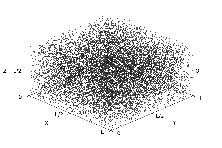
Figure 1: Plot of the spatial distribution of particles for different values of the force constant $K$. The magnitude of the slab depth $\sigma$ is also shown for comparison. (top panel) Free tracers case, corresponding to the choice of parameters $K=0$. (middle panel) Intermediate confinement case, with force constant $K=0.125$. The associated effective slab depth is $\sigma\simeq 21\eta$. (bottom panel) Strong confinement case corresponding to parameters $K=6$ and $\sigma\simeq 0.46\eta$. Here, particles are almost perfectly confined in a plane. The presence of the vertical confinement induces an evident and strong preferential concentration in the horizontal plane.

In Figure 1 we show some representative snapshots of the system, for different values of the force constant $K$. From these pictures it is evident that confinement has strong effects both at large and small scales.

For unconfined particles we observe the classical homogeneous distribution on the whole volume, while in the extreme case of particles bound to move on a plane, we observe a fractal-like distribution with a dimension considerably smaller than $2$. For each different value of the force constant we estimated the probability density of finding a particle with a $z$ coordinate in the range $[z;z+\delta z]$ computing an histogram, $N_{K}(z)$. Figure 2 shows the histograms for the $z$ distribution of the particles. The distribution is well approximated by a Gaussian with center at $z=z_{0}$ and variance $\sigma^{2}$.

Each curve in Figure 2 corresponds to a specific value of $\sigma$. There is a one-to-one correspondence between the values of $\sigma$ and those of the force constant $K$. Measuring $\sigma$ is thus an intuitive way for quantitatively describing the strength of the confinement of the particles around the central plane $z=z_{0}$.

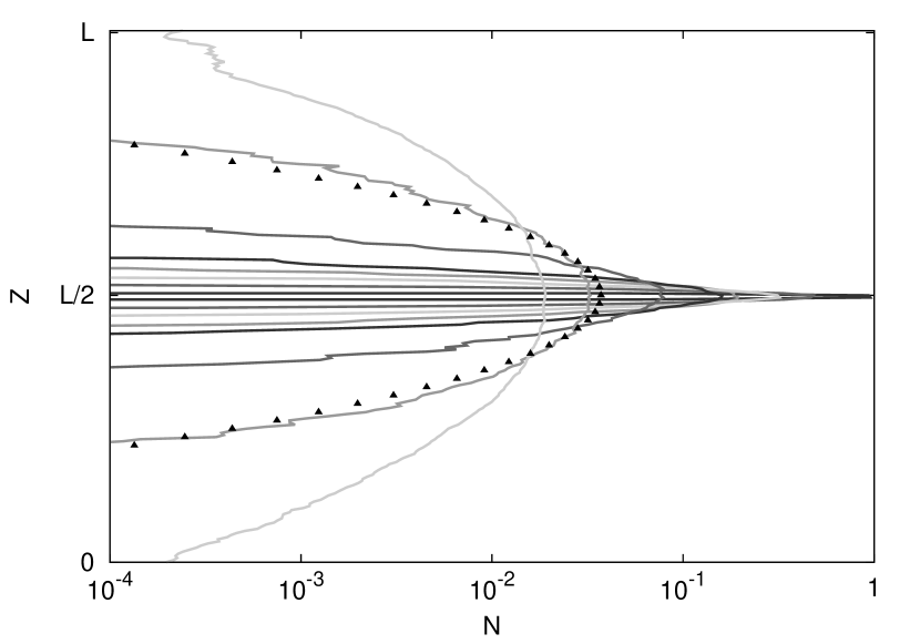
Figure 2: Plot of the normalized $z$-distribution of particles, $N_{K}(z)$, for different values of the force constant $K$ (or different values of $\sigma$). The curves corresponds to the values $\sigma/\eta=38,21,9.1,4.7,3.48,2.33,1.41,0.46$; the vertical width of the distribution monotonically increases. The points show a normalized Gaussian fit for the curve with $\sigma/\eta=21$. $\eta$ is the Kolmogorov length scale.

For a linear restoring force, we expect $\sigma$ to be inversely proportional to $K$. Furthermore, it is possible to calculate analytically the value of $\sigma$ in two limit cases: unconfined particles or particles restricted to a plane. In the limit of particles strictly confined on a plane, i.e., $K\rightarrow\infty$, $\sigma$ is exactly zero. In the limit of $K\rightarrow 0$, i.e., no vertically constraining force, particles are freely advected over the full domain following the underlying fluid motion (3D turbulent diffusion). The particle density becomes homogeneous over the cubic domain and $\sigma$ evolves to a constant value that is a fraction of $L$. Figure 3 shows the relation between the dispersion $\sigma$ and the force constant $K$. We see that, for large values of $K$, $\sigma$ is proportional to ${1}/{K}$, as we expect. This proportionality should disappear when $K$ is decreased.

Figure 3: Plot of the slab depth $\sigma$ versus the inverse of the force constant $1/K$. The horizontal dotted line is the asymptotic value of $\sigma$ for $K\rightarrow 0$. The slab depth is given in units of $\eta$, the Kolmogorov length scale. $1/K$ is given in units of $\tau_{\eta}^{-1}$, where $\tau_{\eta}$ is the Kolmogorov time scale. The diagonal dashed line is obtained from a linear least squares fit.

III.0.2 2D and 3D compressibility

We measured two different compressibilities for the system of particles (the underlying flow is always incompressible): the 2D compressibility based only on the horizontal velocity components and the full 3D compressibility. In both cases, in order to obtain an ensemble average, the compressibility has been calculated averaging on both particles and time. The error is then given by the standard deviation of the mean.

2D compressibility

The 2D compressibility is defined as:

$$C_{2D}=\frac{\left\langle(\sum_{i}{\partial_{i}u_{i}})^{2}\right\rangle}{\left\langle\sum_{i,j}{(\partial_{i}u_{j})^{2}}\right\rangle}\,,$$ (5)

where $i,j=x,y$ and $u$ is the particle velocity.
In the limit $K\rightarrow 0$ we can calculate analytically the value of $C_{2D}$. This limit corresponds to extracting the velocity data from a plane in a fully 3D flow field. For a 3D homogeneous and isotropic turbulent flow (HIT), by simply substituting the relations between the velocity gradients inside Eq. (5), we find $C_{2D}^{HIT}=\frac{1}{6}\simeq 0.167$.

Figure 4: Plot of the 2D compressibility $c_{2D}$ versus the slab thickness $\sigma$. Here, $\sigma$ is given in units of the Kolmogorov length scale $\eta$. Data points are obtained averaging on both time and particles. Errors are the standard deviation of the mean.

Figure 4 shows the relation between the 2D compressibility Eq. (5) and particle dispersion $\sigma$ (that is inversely proportional to the force constant $K$). In the case of unconfined particles we correctly recover $C_{2D}=C_{2D}^{HIT}$. Increasing the confinement, the 2D compressibility has a value lower than $C_{2D}^{HIT}$. This is because the exact value $C_{2D}^{HIT}$ is calculated in an Eulerian framework, averaging the velocity field of the flow in the whole plane, while in our case we use the “Lagrangian” velocity gradients, i.e., the Eulerian velocity gradients measured at the positions of the particles (thus not homogeneously distributed in a plane, due to the presence of preferential concentration). Only without preferential concentration do we expect $C_{2D}=C_{2D}^{HIT}$.

3D compressibility

The 3D compressibility is defined as:

$$C_{3D}=\frac{\left\langle(\sum_{i}{\partial_{i}u_{i}})^{2}\right\rangle}{\left\langle\sum_{i,j}{(\partial_{i}u_{j})^{2}}\right\rangle}\,,$$ (6)

where $i,j=x,y,z$ and $u$ is the particle velocity.
Substituting the equations of motion (II.2) in Eq. (6) we obtain:

$$C_{3D}=\frac{\left\langle(\partial_{x}v_{x}+\partial_{y}v_{y}+\partial_{z}v_{z}-K)^{2}\right\rangle}{\left\langle\left[\sum_{i,j}{(\partial_{i}v_{j})^{2}}\right]-2K\partial_{z}v_{z}+K^{2}\right\rangle}=$$

$$=\frac{K^{2}}{\left\langle\sum_{i,j}{(\partial_{i}v_{j})^{2}}\right\rangle+K^{2}}\,,$$ (7)

where we explicitly used the incompressibility of the 3D flow field and the fact that $\langle\partial_{z}v_{z}\rangle=0$. So we expect $C_{3D}=0$ in the $K\rightarrow 0$ limit, and $C_{3D}=1$ in the $K\rightarrow\infty$ limit.

Figure 5 shows the relation between the 3D compressibility (6) and the particle dispersion $\sigma$ (that is inversely proportional to the force constant $K$). As expected, $C_{3D}$ is zero for tracers, and increases monotonically with the confinement strength.

Figure 5: Log-log plot of the 3D compressibility $C_{3D}$ versus the slab thickness $\sigma$. Here $\sigma$ is given in units of the Kolmogorov length scale $\eta$. The dashed line is a fit of Eq. (III.0.2).

III.0.3 Accumulation of particles and pair correlations in space

Another important way of characterizing the system is to look at the distribution of particles at small scales, i.e., the tendency of particles to inhomogeneously concentrate in space. This behavior is the result of the interplay between the motion induced by the underlying fluid and the presence of a vertically confining force on the particles. Because of the inhomogeneity on the vertical direction, we decided to characterize the spatial distribution centering the analysis on a small volume around the central equilibrium plane:

$$A=\left\{z_{i}\in\left[L/2-\Delta z;L/2+\Delta z\right]\right\}\,,$$ (8)

with $\Delta z\simeq 0.2\eta$. In this way, measurements on horizontal scales larger (smaller) than $\Delta z$ will be mainly two-dimensional (three dimensional).

We defined a pair distribution integral, $P_{2}(r)$ as follows: having defined the set $A$ of all particles falling in the central volume of vertical width $\Delta z$, one counts how many pairs with a relative distance $\leq r$ can be formed with a particle in $A$ and another particle anywhere in the volume. Formally:

$$P_{2}(r)=\sum_{i\in A}\sum^{N_{p}}_{j=1}\Theta(r-\left|\mathbf{x}_{i}-\mathbf{x}_{j}\right|)\,,$$ (9)

where $\Theta(x)$ is the Heaviside step function and $\mathbf{x}_{i}$, $\mathbf{x}_{j}$ are the particle coordinates. If one had chosen $A$ equal to the whole system of particles then one would obtain the classical correlation dimension grassberger1983measuring .

In order to quantify the scale-by-scale clustering properties it is useful to introduce the local scaling-exponent

$$\zeta(r)=\frac{d\log\left(P_{2}(r^{\prime})\right)}{d\log\left(r^{\prime}\right)}\Big{|}_{r^{\prime}=r}\,.$$ (10)

In the limit $r\rightarrow 0$ one expects that the scaling exponent recovers the definition of correlation dimension of the particle distribution.

This local scaling exponent expresses how the number of pairs scales with the distance $r$, for the particles in the innermost part of the layer.

Figure 6 shows the local scaling exponent $\zeta(r)$ versus the radial distance of the pairs, where the error bars have been estimated by comparing results between two different subsets of the whole statistics.

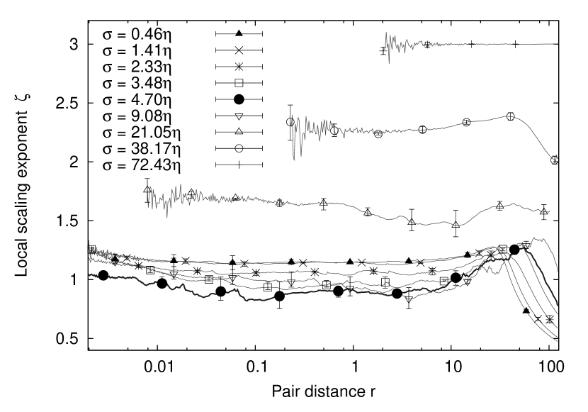
Figure 6: Log-log plot of the local scaling exponents $\zeta(r)$ versus the radial distance of the pairs, for different values of the effective slab thickness $\sigma$. Continuous lines represent all the available data; the purpose of the symbols is to help the reader to distinguish the different curves. Both the slab thickness $\sigma$ and the pair distance $r$ are given in units of the Kolmogorov length scale $\eta$. Only a few indicative error bars are shown, in order to keep the Figure clear. The error bars have been estimated by comparing results between two different subsets of the whole statistics. The curve corresponding to $\sigma=4.70\eta$ is emphasized to stress the fact that the minimum in fractal dimension does not correspond to the minimum in slab thickness.

Figure 7 show the local scaling exponents $\zeta(r)$ at different values of the distance $r$ versus the particle dispersion $\sigma$. This figure confirms the results of Fig. 6: there exists a minimum in the exponent (corresponding to a maximum in the accumulation of particles) for $\sigma\simeq 5\eta$, at least in a range of scales $0.02<r/\eta<19.6$. For $\sigma\gtrsim 5\eta$ the exponent grows, corresponding to a decrease in clustering because of the reduced confinement effects. On the other hand, if $\sigma$ is decreased below $\eta$ the exponent stays constant, since the particles are already constrained to be very close to the central plane.

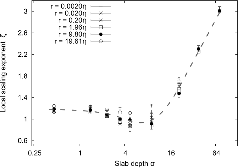
Figure 7: Plot of the value of the power-law exponent $\zeta(r)$ versus $\sigma$ for different values of $r$. We can see that the curves in the range $0.02<r/\eta<19.6$ exhibit non-monotonicity, and a minimum around $r\simeq 5\eta$. Points are taken intersecting the curves in Figure 6 with lines $r={\rm{constant}}$. Both the slab thickness $\sigma$ and the pair distance $r$ are given in units of the Kolmogorov length scale $\eta$. The error estimation procedure is detailed at the end of Sec. III.0.3. The dashed line is merely a guide for the eye.

Let us notice that using the correlation integral as introduced in grassberger1983measuring to analyze the particle distribution leads to an undesirable effect for our set-up: centering the spheres on peripheral particles (far from the central plane), gives a lower number of pairs inside a given sphere of radius $r$ because of the vertical non-homogeneous distribution. Using our definition to measure the pair distribution integral $P_{2}(r)$ corresponds to measuring the original three-dimensional distribution in such a way that the “central” particles have a larger weight with respect to the peripheral ones, and the effect of the inhomogeneity in the $z$ direction is less pronounced. The value $\Delta z\simeq 0.2\eta$ has been chosen because it allows us to shift the abrupt drop in the scaling exponent ( visible in Fig. 6) at large scales, leaving a cleaner power-law behavior at the scales we are interested in. Increasing $\Delta z$ would shift the drop in the scaling exponent at smaller length scales.

IV Conclusions

In this study we have investigated the dynamics of a system of particles suspended in a turbulent flow and vertically constrained to evolve within an horizontal slab with a certain thickness depending on an effective linear restoring force. In particular, we quantified the effective compressibility of the particle distribution and particle accumulation varying the degree of confinement.

Using DNS we have studied a simplified model in which particles are suspended in a 3D, isotropic and homogeneous, turbulent flow. These particles are passive, point-like and confined only in the vertical direction by means of a restoring force. We studied different situations, varying the thickness of the slab, in order to analyze the characteristics of the particle suspension in a range of conditions from having full accessibility to the 3D incompressible flow, to a 2D slice of a 3D incompressible flow. The particle distribution shows a certain degree of compressibility, except for $K\rightarrow 0$.

We have also shown that there exists a particular -optimal- value of the effective slab thickness $\sigma$ (or, equivalently, of the force constant $K$) that maximizes the accumulation of the particles (minimizing the fractal dimension of the system). This happens when the depth of the horizontal slab is of the order of a few Kolmogorov length scales $\eta$ ($\sigma\sim 5\eta$). Let us point out that viscous effects are known to be important up to $5-10\eta$ in turbulent flows, meaning that the maximum particle accumulation is achieved when their vertical displacement is bounded to be no larger than the size of viscous eddies.

We want to stress how our model, though simple, could be important towards the quantitative understanding of the phenomenology of passive, point-like entities in a turbulent marine thin layer. Indeed, our model captures the generic features associated with the presence of a vertical localization, irrespective of the biological or physical reason beyond its production and its stability. Thin phytoplankton layers are always much thicker than the size of individual cells and for this reason one may question how the discussed confinement may be relevant at all to plankton population dynamics. Here it must be stressed that what is important is the relation between time scales, and not length scales, in the system. Indeed the typical generation time for plankton and bacteria in a marine environment is well within the inertial range and such that over a generation the cell has been transported to distances much larger than the vertical confinement. Clearly real marine conditions are complicated by many more phenomena that we have not included in our model and the real plankton dynamics shows phenomena that the simplified model discussed here cannot incorporate. The improvement of our model in order to apply it to more complex situations and to the modeling of systems more similar to real-life plankton particles in oceans is a challenge for future studies. For example, an obvious follow-up to this investigation would be to simulate inertial particles instead of passive tracers, integrating more physically accurate equations of motion, while keeping a simple linear restoring force for the vertical confinement.

References

- [1] M. R. Maxey. The gravitational settling of aerosol particles in homogeneous turbulence and random flow fields. Journal of Fluid Mechanics, 174:441–465, 1987.
- [2] E. Balkovsky, G. Falkovich, and A. Fouxon. Intermittent distribution of inertial particles in turbulent flows. Physical Review Letters, 86:2790–2793, 2001.
- [3] J. Bec. Fractal clustering of inertial particles in random flows. Physics of Fluids (1994-present), 15:L81–L84, 2003.
- [4] J. Bec, L. Biferale, M. Cencini, A. Lanotte, S. Musacchio, and F. Toschi. Heavy particle concentration in turbulence at dissipative and inertial scales. Physical Review Letters, 98:084502, 2007.
- [5] Federico Toschi and Eberhard Bodenschatz. Lagrangian properties of particles in turbulence. Annual Review of Fluid Mechanics, 41:375–404, 2009.
- [6] J. Bec, L. Biferale, M. Cencini, A. S. Lanotte, and F. Toschi. Intermittency in the velocity distribution of heavy particles in turbulence. Journal of Fluid Mechanics, 646:527–536, 2010.
- [7] I. Fouxon. Distribution of particles and bubbles in turbulence at a small stokes number. Physical Review Letters, 108:134502, 2012.
- [8] K. Gustavsson, S. Vajedi, and B. Mehlig. Clustering of particles falling in a turbulent flow. Physical Review Letters, 112:214501, 2014.
- [9] J. Bec, H. Homann, and S. S. Ray. Gravity-driven enhancement of heavy particle clustering in turbulent flow. Physical Review Letters, 112:184501, 2014.
- [10] K. D. Squires and J. K. Eaton. Preferential concentration of particles by turbulence. Physics of Fluids A: Fluid Dynamics, 3:1169, 1991.
- [11] L. P. Wang and M. R. Maxey. Settling velocity and concentration distribution of heavy particles in homogeneous isotropic turbulence. Journal of Fluid Mechanics, 256:27–27, 1993.
- [12] G. Falkovich, A. Fouxon, and M. G. Stepanov. Acceleration of rain initiation by cloud turbulence. Nature, 419:151–154, 2002.
- [13] R. A. Shaw. Particle-turbulence interactions in atmospheric clouds. Annual Review of Fluid Mechanics, 35:183–227, 2003.
- [14] W. W. Grabowski and L. P. Wang. Growth of cloud droplets in a turbulent environment. Annual Review of Fluid Mechanics, 45:293–324, 2013.
- [15] K. D. Squires and H. Yamazaki. Preferential concentration of marine particles in isotropic turbulence. Deep Sea Research Part I: Oceanographic Research Papers, 42:1989–2004, 1995.
- [16] W. M. Durham, E. Climent, M. Barry, F. De Lillo, G. Boffetta, M. Cencini, and R. Stocker. Turbulence drives microscale patches of motile phytoplankton. Nature Communications, 4(2148), 2013.
- [17] P. Perlekar, R. Benzi, D. R. Nelson, and F. Toschi. Cumulative compressibility effects on slow reactive dynamics in turbulent flows. Journal of Turbulence, 14:161–169, 2013.
- [18] F. De Lillo, M. Cencini, W. M. Durham, M. Barry, R. Stocker, E. Climent, and G. Boffetta. Turbulent fluid acceleration generates clusters of gyrotactic microorganisms. Phys. Rev. Lett., 112:044502, Jan 2014.
- [19] A. P. Martin. Phytoplankton patchiness: the role of lateral stirring and mixing. Progress in Oceanography, 57:125–174, 2003.
- [20] W. M. Durham and R. Stocker. Thin phytoplankton layers: characteristics, mechanisms, and consequences. Annual Review of Marine Science, 4:177–207, 2012.
- [21] W. J. McKiver and Z. Neufeld. Influence of turbulent advection on a phytoplankton ecosystem with nonuniform carrying capacity. Physical Review E, 79:061902, 2009.
- [22] P. Perlekar, R. Benzi, D. R. Nelson, and F. Toschi. Population dynamics at high reynolds number. Phys. Rev. Lett., 105:144501, Sep 2010.
- [23] P. Perlekar, R. Benzi, D. R. Nelson, and F. Toschi. Statistics of population dynamics in turbulence. Journal of Physics: Conference Series, 318(9):092025, 2011.
- [24] D.R. Nelson. Biophysical dynamics in disorderly environments. Annual Review of Biophysics, 41(1):371–402, 2012. PMID: 22443987.
- [25] S. Pigolotti, R. Benzi, M. H. Jensen, and D. R. Nelson. Population genetics in compressible flows. Phys. Rev. Lett., 108:128102, Mar 2012.
- [26] R. Benzi, M. H. Jensen, D. R. Nelson, P. Perlekar, S. Pigolotti, and F. Toschi. Population dynamics in compressible flows. The European Physical Journal Special Topics, 204(1):57–73, 2012.
- [27] S. Pigolotti, R. Benzi, P. Perlekar, M. H. Jensen, F. Toschi, and D. R. Nelson. Growth, competition and cooperation in spatial population genetics. Theoretical Population Biology, 84(0):72 – 86, 2013.
- [28] J. Kalda, T. Soomere, and A. Giudici. On the finite-time compressibility of the surface currents in the gulf of finland, the baltic sea. Journal of Marine Systems, 129(0):56 – 65, 2014.
- [29] M. van Aartrijk and H. J. H. Clercx. Dispersion of heavy particles in stably stratified turbulence. Physics of Fluids, 21:033304, 2009.
- [30] M. van Aartrijk and H. J. H. Clercx. Vertical dispersion of light inertial particles in stably stratified turbulence: The influence of the basset force. Physics of Fluids, 22:013301, 2010.
- [31] AG Lamorgese, DA Caughey, and SB Pope. Direct numerical simulation of homogeneous turbulence with hyperviscosity. Physics of Fluids (1994-present), 17(1):015106, 2005.
- [32] Martin R Maxey and James J Riley. Equation of motion for a small rigid sphere in a nonuniform flow. Physics of Fluids, 26:883, 1983.
- [33] T. R. Auton, J. C. R. Hunt, and M. Prud’Homme. The force exerted on a body in inviscid unsteady non-uniform rotational flow. Journal of Fluid Mechanics, 197:241–257, 1988.
- [34] A. E. Gill. Atmosphere-ocean Dynamics. Academic Press, 1982.
- [35] P. Grassberger and I. Procaccia. Measuring the strangeness of strange attractors. Physica D: Nonlinear Phenomena, 9:189–208, 1983.