A Multiscale Method for Porous Microstructures
Abstract
In this paper we develop a multiscale method to solve problems in complicated porous microstructures with Neumann boundary conditions. By using a coarse-grid quasi-interpolation operator to define a fine detail space and local orthogonal decomposition, we construct multiscale corrections to coarse-grid basis functions with microstructure. By truncating the corrector functions we are able to make a computationally efficient scheme. Error results and analysis are presented. A key component of this analysis is the investigation of the Poincaré constants in perforated domains as they may contain micro-structural information. Using a constructive method originally developed for weighted Poincaré inequalities, we are able to obtain estimates on Poincaré constants with respect to scale and separation length of the pores. Finally, two numerical examples are presented to verify our estimates.
1 Introduction
Modeling and simulation of porous media has many wide ranging applications in engineering. For example, to simulate heat or electric conductivity in complicated materials or composites a partial differential equation (PDE) in complicated microstructures must be solved. Direct numerical simulation of such problems is difficult, and, in some scenarios is intractable. The main challenge being the many scale nature of the problem and complex geometries involved. In these applications, where there are many scales and complex heterogeneities, numerical homogenization procedures are employed to reduce complexity yet remain accurate. In this work, we develop a multiscale method to simulate Neumann problems in domains with porous microstructures.
The study of multiscale problems in porous or perforated domains has a long history. In the area of homogenization of partial differential equations, there is a vast literature on the subject [7, 22, 26] and references therein, to name just a few. In these problems, the fine-scale equations have microstructure, then through an averaging process of homogenization an effective PDE is derived. In these methods, the strong assumption of periodicity is usually made, and thus, only one microstructure dependent local problem is solved to compute effective properties. The coarse-grid, or homogenized problem, does not have explicit microstructure. More computationally based procedures have also been investigated. Using an approach based on the Heterogeneous Multiscale Method [2], an algorithm was developed in [14] by solving for an unknown diffusion coefficient on the coarse-grid by resolving a local perforated domain problem. Then, computation on the coarse-grid equation is based in an effective non-porous domain. Further work, [6], developed a perforated multiscale finite element method for Dirichlet problems utilizing Crouzeix-Raviart non-conforming finite elements. Using the MsFEM framework [8], a weak Crouzeix-Raviart boundary condition is used to construct the multiscale finite element basis that include the vanishing Dirchlet condition into the basis functions. There are also mesoscopic schemes that relax the resolution condition of standard finite elements insofar as they allow that mesh cells are cut by the domain boundary; see e.g. [4, 5, 9, 10, 18] among many others. However, for those schemes there are typically strong restrictions on the topology of the intersection that rule out the case of perforation on the element level.
We will work in the multiscale framework using a local orthogonal decomposition (LOD) [21], which is inspired by the variational multiscale method [17, 16, 19]. The LOD method uses a coarse-grid quasi-interpolation operator to decompose the space into fine-scale components to build the fine detail space. From the fine detail space we are able to build multiscale corrections to the coarse-grid functions and construct a multiscale space. These corrections have global support, thus limiting their practical usage. However, these corrections have fast decay and can therefore be localized. This procedure has been used effectively for elliptic problems with coefficients [12, 15, 21], been extended to semi-linear elliptic equations [13], linear and nonlinear eigenvalue problems [11, 20], and to the wave equation [1].
In this work, we extend this framework to the case when we have microstructures that generate the multiscale features as opposed to oscillatory and highly varying coefficients. We first build a coarse-perforated grid, then by using a quasi-interpolation operator based on local projection build a fine-scale space. We again follow the process in [12, 15, 21] of multiscale space construction, localization, and subsequent error estimates. We show that we can obtain the same error estimates with respect to coarse-grid size and truncation of local problems as in these works. However, in this setting we are particularly concerned with the tracking of Poincaré constants in perforated domains as these may depend on the micro-structural features, namely the size of particles and separation length. Using the methods developed in [24], originally for the setting of high-contrast coefficients and weighted Poincaré inequalities, we are able to create a constructive procedure to estimate these constants in domains with microstructure. This is carried out for a few interesting examples. We show that in the case of a reticulated filamented structure it is possible that the microstructural features can negatively impact this Poincaré constant in the case of very thin structures. In addition, we show that in the case of isolated particles we obtain uniform (microstructure independent) Poincaré constants.
The paper is organized as follows. We begin by the problem setting and the description of quasi-interpolations in perforated domains. This quasi-interpolation will allow us to construct our multiscale orthogonal splitting and subsequent computational localization algorithm. Then, we will derive error estimates on both global supported and localized basis functions. This is done with the help of technical lemmas in the Appendix and careful tracking of relevant constants. We then develop a constructive procedure to estimate Poincaré constants in porous domains. Finally, we give two numerical examples to demonstrate the rates of convergence with respect to mesh parameters, localization truncation, and microstructure lengths. In addition, we discuss overall effectiveness of the algorithm and the choices of possible quasi-interpolation operators.
2 Problem Set Up
We now begin with some notation and problem setting. Let be a bounded Lipschitz domain with polyhedral boundary for . We denote the solid microstructure to be , a set of Lipschitz nonintersecting closed subsets of . We denote the perforated domain, often called fluid or porous domain, , where . We supposed that the solid microstructure or inclusions are so that remains connected and Lipschitz. We let be the characteristic size of the microstructure.
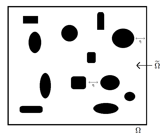
Moreover, we let also be the minimal separation length. These two parameters may be considered separately, but for clarity we choose them to be on the same order of magnitude. We suppose for simplicity that the perforations do not intersect the global boundary, but may be close to it. An example geometry can be seen in Figure 1.
We wish to find a solution that satisfies
| (1a) | ||||
| (1b) | ||||
| (1c) | ||||
Where , and denotes the outer normal on
We denote the space . Multiplying by and integrating (1), we wish to solve for such that
| (2) |
here is the standard real Lebesgue measure in . The main difficulty in solving the above problem is the mutliscale nature introduced from the microstructure. We may also add in an oscillatory coefficient inside the perforated domain , however, this case is well studied in [21] and we focus on the issues involved with the multiscale geometries.
3 Quasi-Interpolation in Perforated Domains
In this section we develop the framework to work on perforated domains. We first define the classical nodal basis restricted to the perforated domain. Then, we describe how to construct a quasi-interpolation that is also projective, in contrast to the quasi-interpolation operator used in [21].
3.1 Classical Nodal Basis
Following much of the notation in [21], suppose that we have a coarse quasi-uniform discretization of the unperforated domain with mesh size . We denote the interior nodes not on the boundary of the coarse mesh as . Let the classical conforming finite element space over be given by , and let . We denote the nodal basis functions , that is for an interior node , we have
| (3) |
This is a basis for . Let be the function satisfying
To move to the perforated domain it is useful to have some more notation. We denote the restriction operator of a function on to by . We denote the space of finite element functions (3) restricted to the perforated domain as
From here we may define a coarse-grid variational form of (2). Indeed, let be the function satisfying
| (4) |
However, will not be a good approximation to unless is sufficiently small to resolve the microstructure.
3.2 Projective Quasi-Interpolation
In this section, we develop the theory for a quasi-interpolation operator that is also a projection. This projective quasi-interpolation gives stability properties required for the localization theory without the use of an auxiliary ”closeness to projection” lemma used in the theory of Clément quasi-interpolation theory c.f. Lemma 1 of [12]. This requires the construction of a function that satisfies certain interpolation properties and derivative bounds. However, in the case of perforated domains such a construction can be quite tedious and an alternate approach is utilized here.
We will construct a quasi-interpolation operator that is also projective and satisfies the requisite local stability properties. For non-perforated domains, this is a well known modification of the operator of Clément [23]. We denote the local patch for and, subsequently, the perforated patch as . First, we define the local patch projection as the operator such that for
| (5) |
From this we define the interpolation operator for as
| (6) |
Given a function with support contained in a patch of triangles , then, by the definition of the quasi-interpolation (6), it is clear that in general, as the boundary nodes on the patch will add a contribution smearing out the function. To deal with this issue we require some notation and definitions. Using the definition and notation in [12], we define for any patch the extension patch
| (7a) | ||||
| (7b) | ||||
for . With this notation we have if for the interpolator (6).
We have the following stability and local approximation of the quasi-interpolation operator defined by (6), along with the desired projective properties.
Lemma 3.1
There exists a constant , for all , such that
| (8) |
where . Here is the Poincaré constant in perforated domains. Here, is a benign constant not depending on or . Moreover, the interpolation is a projection.
-
Proof
See Appendix A.
It is important to note that we have a Poincaré constant in the above estimate. Since our domain can have complicated microstructure we must be careful when analyzing estimates that contain this constant. We suppose that we have the following general Poincaré inequality for each patch for . Moreover, we shall suppose that this constant serves as a global bound with respect to and . The analysis of such a constant will be considered in Section 6.
For all with , we have for
| (9) |
Where may depend on the diameter of the triangulation, and subsequently , and its characteristic microstructure parameter . We denote and will drop the notation in many of the auxiliary estimates in the Appendix B and throughout the paper when there is no ambiguity.
4 Multiscale Splitting and Basis
We now will construct our multiscale approximation space to handle the oscillations created by the perforated microstructure. The main ideas of this splitting can be found in [12, 21] and references therein. As noted before the coarse mesh space restricted to can not resolve the features of the microstructure and these fine-scale features must be captured in the multiscale basis. We begin by constructing fine-scale spaces.
We define the kernel of the perforated interpolation operator to be
where is defined by (6). This space will represent the small scale features not captured by . We define the fine-scale projection to be the operator such that for we compute as
| (10) |
This projection gives an orthogonal splitting with We can decompose any as with . This modified coarse space is referred to as the multiscale space and contains fine-scale geometric information. The multiscale Galerkin approximation satisfies
| (11) |
To construct the basis for the multiscale space we construct an adapted coarse grid basis. We define the corrector to be the solution to
| (12) |
We then define the perforated multiscale space to be the functions spanned by
| (13) |
Note that the corrector problem (10) is posed on the global domain. Thus, the corrections will have global support and as such have limited practical use. However, in the following analysis we show that the basis can be localized.
The key issue with constructing the solution to (11) is the calculation of the corrector on a global basis. However, it can be shown that the corrector decays exponentially fast. To this end, we define the localized fine-scale space to be the fine-scale space extended by zero outside the patch, that is . It is convenient to introduce some notion here similar to that introduced in [12]. We let for some and the local corrector operator be defined such that given a
| (14) |
where is augmented so that the collection is a partition of unity. This is done because the Dirchlet condition makes the standard basis not a partition of unity near the boundary. For a practical evaluation of , we may precompute for any neighbor of the following
| (15) |
We then write and so must only compute over small number of nearby nodes for each . Moreover, we are able to exploit local periodic structures due to the fact that a drastically reduced number of corrector problems must be computed, assuming the coarse-grid is chosen properly.
We denote the global corrector operator as
With this notation, we write the truncated multiscale space as
Moreover, note also that for sufficiently large , we recover the full domain and obtain the ideal corrector with functions of global support, denoted The corresponding multiscale approximation to (2) is
| (16) |
5 Error Analysis
In this section we present the error introduced by using (11) on the global domain to compute the solution to (2). Then, we show how localization effects the error when we use (16) on truncated domains to compute the same solution. Meanwhile, we must carefully account for the effects of the Poincaré constant from (9) in the estimate as in certain domains this may depend on the microstructure or coarse grid diameters.
5.1 Error with Global Support
Theorem 5.1
-
Proof
Again we use the local stability property of the local interpolation operator in (36). From the orthogonal splitting of the spaces it is clear that and . Thus, using the stability inequality we have
Let be the maximal number of elements covered by a patch and we suppose the mesh is so that this is uniformly bounded. Taking we arrive at the estimate (19).
5.2 Error with Localization
In this section we show the error due to truncation with respect to patch extensions. The key lemma needed is the following estimate, the proof can be found in Appendix B.
Lemma 5.2
Let , let be constructed from (14), and defined to be the ”ideal” corrector without truncation, then
| (18) |
with , and .
The lemma gives the decay in the error as the truncated corrector approaches the ideal corrector of global support. With this lemma we are able to state and prove Theorem 5.3.
Theorem 5.3
- Remark
6 Estimates for Poincaré Inequalities
In this section, we discuss the tools required to estimate the constant in certain physically interesting cases. The following techniques were developed and used effectively in the context of weighted Poincaré inequalities in the setting of contrast dependence [24] and references therein. We follow much of the notation presented in that work, however, here we adapt the techniques to complex domain geometries and not contrast independent estimates. The case of high-contrast will be discussed in the forthcoming preprint [25]. We begin by building the necessary framework to effectively estimate in a constructive way. Throughout this section we shall suppose that , the characteristic separation and length scale size.
We begin by fixing and examining a single patch . We will have a slight abuse of notation we call this constant Poincaré as we will take a maximum over all patches. We suppose that the estimate on this patch bounds all the others. We begin as in [24], let be a non overlapping partitioning of into open, connected Lipschitz polytopes so that
with For and dimensional manifold we define the average
here the above integral is taken with respect to the dimensional real Lebesgue measure .
We call a region a path if for each , the regions and share a common -dimensional manifold. Here, is the length of the path . Suppose there is a path from to with path length . Let be a dimensional manifold, then for each let be the best constant so that
| (20) |
for all . Note here we make a change of notation compared to [24], in that we replace with its square, similarly with and related constants.
We now define the Poincaré inequality for a single domain, most likely in our application to be a simplicial domain such as a triangle, tetrahedron, or perhaps nonsimplicial, but regular, such as quadrilaterals, parallelepiped, or curved elements. The key here being that each simplex has a trivially bounded Poincaré constant. For any Lipschitz domain and for any dimensional manifold , we denote to be the best constant such that
| (21) |
for all . We have the following lemma relating the constants in (20) and (21).
Lemma 6.1
| (22) |
-
Proof
By using the standard telescoping argument
and the use of (21) we have
Fixing we have for the second term
A final application of the Cauchy inequality yields the desired result.
We define and we have the general full Poincaré inequality
| (23) |
recall here is the optimal minimizing constant.
6.1 Poincaré Inequalities with Geometric Parameters
To obtain better bounds on we must in turn obtain a systematic way to obtain bounds on . To this end, we will use the following two technical lemmas. The first of which estimates the constant for a simplex.
Lemma 6.2
Let be a simplex (or parallelepiped), and one of its faces, then
-
Proof
See Appendix of [24].
We also state a common estimate for regular triangulation.
Lemma 6.3
Let a nondegenerate simplex and the diameter of the largest sphere inscribed in , then
-
Proof
See Appendix of [24].
Let be a conforming simplicial triangulation of and we define the geometric parameters for , , , and . We define the shape-regularity constant
We call a partition of shape regular if there is a uniform bound for and quasi-uniform if in addition to shape regular we have uniformly bounded. With this type of a partition we are able to obtain a useful tool to estimate .
Lemma 6.4
Let be a shape regular simplicial partition of , with a facet of . We denote the path length for to by . Then, we have the bound
| (24) |
- Proof
As noted in [24], the above lemma can give ”worst case” scenarios for estimates on Poincaré constants. To illustrate the usefulness of the above estimate (24) to obtain rough bounds we give an illustrative example. It can be easily seen that the estimate (24) will grow when the path lengths, , are large. This can be especially bad in highly tortuous microstructures. We illuminate this by considering a two-dimensional filamented microstructure.
Suppose we take our domain to be , and inside we have the solid microstructure, , given by thin filamented structures. More precisely,
where . Note we take here the floor of to ensure is such that we have the right hand side boundary free of microstructure intersections. This is done since we will suppose that and we wish this boundary to be a part of the domain defined as
Suppose we have a uniform shape regular triangularization of denoted again by . Moreover, we suppose that , for all . We denote the maximal path length from to . Then, (24) becomes
| (25) |
here is a benign constant. To estimate , we take the simplex farthest from the right hand side boundary denoted to construct the longest path. Note that is formed by bisecting into two equal triangles and taking the one adjacent to the left boundary of . We can see that in each filament the path length is and there are filaments. Hence , and in addition, we see also that as this is the number of triangles in the partition of . We thus obtain the estimate for the Poincaré constant
| (26) |
Taking the maximum over the possible constants over the patches, and applying this estimate to Theorem 5.3 we have
| (27) |
Thus, it is possible to see how the closeness of the microstructure could theoretically effect the convergence estimate via the Poincaré. The constant in the exponential may also effect the decay with respect to patch extension. However, the above example is meant to represent a very poor scenario.
-
Remark
It is important to note here that the above estimate holds for . The Poincaré constants in the other regimes would certainly not be expected to yield a convergence order of more than in a regime such as . In this regime, where scale separation is not the case, the notation would be more appropriate.
6.2 Poincaré Constants for Isolated Perforations
In the previous section, we presented a general method for determining the dependence of the Poincaré constant on the microstructure. This estimate offers a sort of worst case scenario for such a constant. In this section, we will show that for isolated convex particles in two-dimensions fairs much better and in fact can be shown to be uniformly bounded. To this end we will need some further results again drawn from the work of [24].
Lemma 6.5
Let be a shape regular and quasi-uniform simplicial partition of with mesh size . Further, let , where are the faces of and for simplicity suppose is not perforated. For and we denote the path from to . Then, we have the bound
| (28) |
for all and where is the path length of .
- Proof
Now we are able to obtain an alternative estimate approach compared to Lemma 6.4.
Lemma 6.6
Assuming the assumptions of Lemma 6.5, we let and path . Then, we have the estimate
| (29) |
here and
is the maximal number of times any simplices is in a path.
-
Proof
Without loss of generality we suppose for that . Using the identity, for (note here is a dimensional variable) and integrating we have
The middle term vanishes and we have
Using Lemma 6.5, we have
Dividing by completes the argument.
With the above lemmas we are able to obtain uniform bounds for isolated perforations. To illuminate the ideas needed to obtain such bounds, we propose a simple example. Again, as before, we suppose we have . For simplicity of the exposition, we define the perforation solids as periodic square domains. More specifically we define the solid domain to be
here is chosen so that the top and right boundaries of are not intersected. We let be a quasi-uniform and shape regular partition of with mesh size . We let be the right boundary and the faces of some elements in the partition. Thus, we have . Since the particles are size and the minimal spacing is size there always exists a path from to some face for some such that In addition, it is also easy to see that . Using the estimate in Lemma 6.6 we have
| (30) |
or a uniform bound on the Poincaré constant for these isolated particles.
-
Remark
We note here that the periodicity of the particles is not at all essential on the above bound. Also the shape may be easily extended to convex and shape regular (i.e. not too oblique) isolated particles. The key parts being the ability to construct path lengths of order We summarize this fact in a Corollary.
Corollary 6.7
Suppose we have a collection of isolated convex shape-regular particles with characteristic size and distance . Moreover, suppose that and for some quasi-uniform and shape regular partition , with mesh size of . Then, the Poincaré constant is uniformly bounded
| (31) |
where does not depend on or .
7 Numerical Examples
In this section we will present a two numerical examples. We apply our algorithm to (1) using our multiscale method and compare with standard finite elements. Using a penalization method, we will implement the micro-structural features into the domain. We will do this for two relevant examples. The first being a periodic square domain with square particles, and the second an dumbbell-shaped domain containing the microstructure of the first experiment. We will demonstrate the validity of our estimates based on varying patch size (truncation of the localization) and by varying microstructure lengths . When we vary the microstructure lengths we will also fix our truncation patch parameter to be proportional to
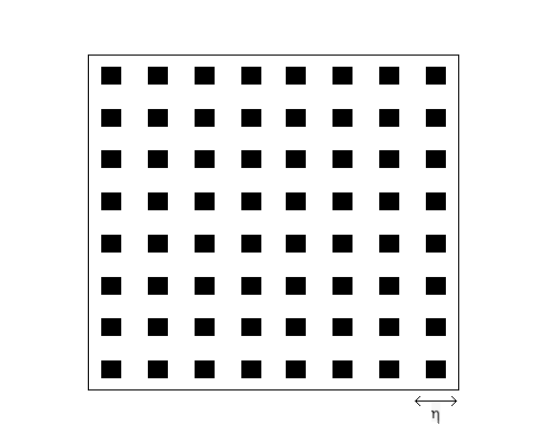
We begin by describing the geometry of the domains. First, we take our unperforated domain to be and define the unit cell to be . We define the perforated domain to be
| (33) |
where is chosen so that the domain is periodically tessellated. This domain for can be seen in Figure 2.
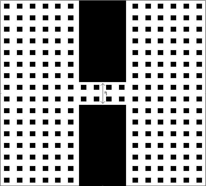
Since this geometry will clearly be in the same class as the uniform bound estimate (31), we choose our second geometry to be an dumbbell-shaped domain. As noted in [24], such a shaped domain has a theoretical bound . Here is the separation of the narrowest part of the domain. More concretely, we let
In addition to the structure we also take out some of the square perforations as in (33) for a fixed period of . We define the following domain
| (34) |
this domain can be seen in Figure 3. Note here, the size of the perforations are fixed and the varying quantity is the size of the narrowest part of the domain in the middle strip.
To solve the problems in the porous domains, we will explicitly grid the perforations on the fine scale, not on the coarse scale. A penalization scheme could also be utilized to relax the restrictiveness of gridding the fine scale. Note, there is a fine scale to solve the local problems and we take this value to be . For all the following examples we will use the forcing
In addition to using the projective quasi-interpolation operator (6), we also present results from the Clément interpolation operator [21],
| (35) |
where . Recall, we chose the projective quasi-interpolator only to simplify the proofs, and here we present numerical results to show that, in these cases, good results hold for the Clément interpolation operator also.
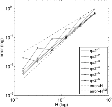
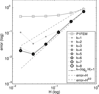
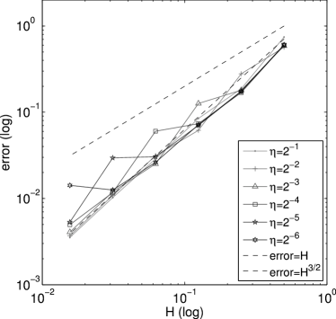
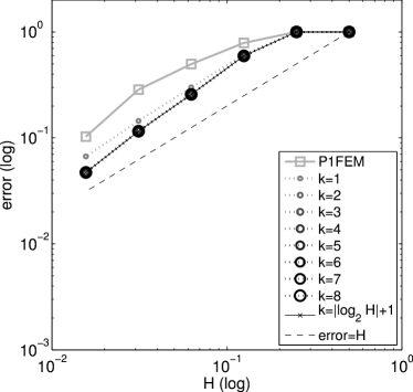
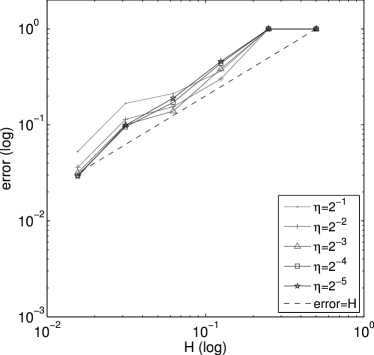
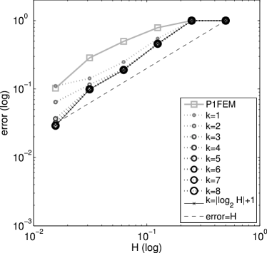
We present results for both media (33) and (34) while using both interpolation operators (6) and (35). We have two types of numerical tests. First, varying the microstructure parameter while keeping the -patch growth fixed to . The idea here to see the effect of the error estimates from the possibly error degrading Poincaré constant. Second, we fix the microstructure length to the smallest value and vary the patch size to observe the rates of exponential convergence. All of these results are compared against an ”overkill” fine-scale solution with in the norm.
The results from the geometry (33) are contained in Figure 4 and 5. In Figure 4, we use the projective interpolator (6) and in Figure 5 we use the Clément interpolator (35). Varying the microstructure, in the case period size , while fixing the patch extension we plot the results for both interpolators in Figure 4a and Figure 5a. In both examples we see that the Poincaré constant does not effect the estimate negatively in agreement with (31). In Figure 4b and Figure 5b we fix the geometric parameter to the smallest value and vary the patch size parameter . We note that the slightly more expensive projective quasi-interpolator, as it requires many local projections, performs better in this case at exponential convergence of the patch extensions.
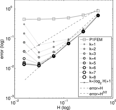
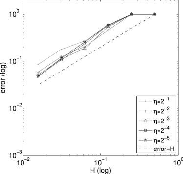
The results from the geometry (34) are contained in Figure 6 and 7. In Figure 6, we use the projective interpolator (6) and in Figure 7 we use the Clément interpolator (35). Keeping the period fixed but varying , the width of the thinnest part, and again fixing the patch extension we plot the results for both interpolators in Figure 6a and Figure 7a. In Figure 6b and Figure 7b we fix the geometric parameter to the smallest value and vary the patch size parameter . Again we see slightly better performance with respect to exponential convergence of the patch extensions for the projective quasi-interpolation.
8 Conclusion
In this work we developed a multiscale procedure to compute Laplacian problems with zero Neumann data in domains with complicated porous microstructure. We are were able to determine the error with respect to the ideal corrector and error due to truncation and localization of the multiscale correctors. As was noted, keeping track of Poincaré constants was critical in our analysis as they may contain information about the microstructure. We used a constructive procedure to estimate these constants and obtain bounds with respect to and . This procedure was demonstrated on two interesting examples. Finally, we implemented numerical tests to validate our theoretical estimates. We found our numerical experiments were in agreement with the theory and the quasi-interpolator based on local projections to perform slightly better than the Clément type.
Appendix A Quasi-Interpolation Stability
We now will prove the stability estimate used throughout for this projective quasi-interpolation operator (6). The proof of this lemma is based on that presented in [23].
Lemma A.1
For , there exists a constant , such that
| (36) |
where . Here is the Poincaré constant and is a benign constant not depending on or . Morever, the interpolation is a projection.
-
Proof
Note that we have easily from this definition taking and applying Cauchy-Schwarz thus, . We use , here again the fact that the projection of a constant is itself, and the fact that is also a projection we obtain
(37) Here, we used the inequality (9) to obtain the gradient bound. To obtain the derivative bound note that by a use of the inverse inequality and (9) we have
(38) This is merely the stability of the projection c.f. [3] and references therein.
We suppose that the basis functions form a partition of unity, that is . We are only proving for the elements that do not meet the boundary. If the elements meet the boundary the Friedrichs’ inequality can be utilized. Thus, we have for the norm
| (39) |
We can easily estimate the first term by using (37), taking a closer look at the second term, again using the partition of unity property, we have
Returning to (39), we have
| (40) |
Using the estimate (38), and a similar argument as above for the estimate [23], we obtain the derivative estimate
| (41) |
To see the is a projection note for , the local patch projection, acting on is a projection, and moreover is identity. By definition we have
| (42) |
and thus it is trivial to see on for all . Thus,
and so and so by linearity
From here we see that .
Appendix B Auxiliary Lemmas
Now we will prove and state the auxiliary lemmas used to prove estimate (19). These proofs are largely based on the works [12, 21] and references therein. However, here we must carefully track the occurrence of Poincaré constants.
First, we begin with the quasi-incusion property. For and and with we have if
| (43) |
We will use the cutoff functions defined in [12]. For and , let be a continuous weakly differentiable functions so that
| (44a) | ||||
| (44b) | ||||
| (44c) | ||||
A precise form of can be written as
If , then we prescribe .
Unlike in [12], we are using a quasi-interpolation that is also a projection. This simplifies the proofs since there is no need to construct an approximate projection. Here we will need the following simplified quasi-invariance of the fine-scale space under multiplication by cutoff functions. We write this estimate in the following lemma.
Lemma B.1
Let and . Suppose that , then we have the estimate
| (45) |
here .
-
Proof
Fixing and , we denote the average as We estimate on a single patch , using the fact that and the estimate (36) we have
Summing over all , using the quasi-inclusion property (43), and the above calculation yields
Noting that only in and only if intersects hence we obtain the tighter estimate
Using the Lipschitz bound on the first term and (36) on the second we obtain
Finally, taking another layer on the outside and inside of the annulus patch we arrive at
here , and note that .
We now will demonstrate the decay of the fine-scale space in the next lemma.
Lemma B.2
Fix some and the dual of satisfying for all . Then, for the solution of
| (46) |
Then, there exists a constant such that for we have
| (47) |
We have , here
-
Proof
Letting be the cut-off function as in the previous lemma for . Let , and note that from Lemma B.1 we have
(48) from this estimate and the properties of we have
(49) We have via Caccioppoli type argument that
(50) (51) Using the fact that , estimate (48), and the relation (49) we have
On the last term we used the projection estimate (36) and here Note here that this is the benign constant from the estimate of Taking and successive applications of the above estimate yields
Finally, taking yields the result.
We now are ready to state our result on the error introduced from localization. The heart of this argument is to estimate the error between the truncated corrector constructed, after summing over from (14) and the ideal corrector when is large enough so that we obtain .
Lemma B.3
Let , let be constructed from (14), and defined to be the ”ideal” corrector without truncation, then
| (52) |
with and .
-
Proof
Recall that with
(53) For all , and letting . Note that for , we have . Let and choose a such that . We have and so Thus, satisfies the conditions of Lemma B.2.
Choosing , we have that . We denote subsequently . Taking the cut-off function we have
(54) (55) Estimating the right hand side of (54) for each we have
As in the proof of Lemma B.2, Letting be large enough so that , then and so we have
(56) We have now the estimate for (55) for using the above identity and (48)
Combing the estimates for (54) and (55) we obtain
(57) supposing the , as is guaranteed by quasi-uniformity of the coarse grid. Here we have . To estimate we use the Galerkin orthogonality of the local problem, that is
(58) Taking , we have
Using Lemma B.1 and Lemma B.2 on the second term we arrive at
Combining this estimate into (57) we arrive at the final estimate that
Here we used and denoted .
Appendix C References
References
- [1] A. Abdulle and P. Henning. Localized orthogonal decomposition method for the wave equation with a continuum of scales. ArXiv e-print 1406.6325, 2014.
- [2] Assyr Abdulle, Weinan E, Björn Engquist, and Eric Vanden-Eijnden. The heterogeneous multiscale method. Acta Numer., 21:1–87, 2012.
- [3] R. E. Bank and H. Yserentant. On the H1-stability of the L2-projection onto finite element spaces. Numerische Mathematik, 126(2):361–381, 2014.
- [4] John W. Barrett and Charles M. Elliott. A finite-element method for solving elliptic equations with Neumann data on a curved boundary using unfitted meshes. IMA J. Numer. Anal., 4(3):309–325, 1984.
- [5] Peter Bastian and Christian Engwer. An unfitted finite element method using discontinuous Galerkin. Internat. J. Numer. Methods Engrg., 79(12):1557–1576, 2009.
- [6] Claude Le Bris, Frédéric Legoll, and Alexei Lozinski. An MsFEM type approach for perforated domains. Multiscale Model. Simul., 12(3):1046–1077, 2014.
- [7] G. A. Chechkin, A. L. Piatniski, and A. S. Shamev. Homogenization: Methods and Applications, volume 234 of Translations of Mathematical Monographs. American Mathematical Society, Providence, RI, 2007.
- [8] Y. Efendiev and T. Hou. Multiscale Finite Element Methods: Theory and Applications, volume 4 of Surveys and Tutorials in the Applied Mathematical Sciences. Springer, New York, NY, 2009.
- [9] Stefano Giani and Paul Houston. -adaptive composite discontinuous Galerkin methods for elliptic problems on complicated domains. Numer. Methods Partial Differential Equations, 30(4):1342–1367, 2014.
- [10] W. Hackbusch and S. A. Sauter. Composite finite elements for the approximation of PDEs on domains with complicated micro-structures. Numer. Math., 75(4):447–472, 1997.
- [11] P. Henning, A. Målqvist, and D. Peterseim. Two-level discretization techniques for ground state computations of bose-einstein condensates. SIAM J. Numer. Anal., 52(4):1525–1550, 2014.
- [12] P. Henning, P. Morgenstern, and D. Peterseim. Multiscale Partition of Unity. In M. Griebel and M. A. Schweitzer, editors, Meshfree Methods for Partial Differential Equations VII, volume 100 of Lecture Notes in Computational Science and Engineering. Springer, 2014. Also available as INS Preprint No. 1315.
- [13] Patrick Henning, Axel Målqvist, and Daniel Peterseim. A localized orthogonal decomposition method for semi-linear elliptic problems. ESAIM: Mathematical Modelling and Numerical Analysis, eFirst, 12 2013.
- [14] Patrick Henning and Mario Ohlberger. The heterogeneous multiscale finite element method for elliptic homogenization problems in perforated domains. Numer. Math, pages 601–629.
- [15] Patrick Henning and Daniel Peterseim. Oversampling for the Multiscale Finite Element Method. Multiscale Model. Simul., 11(4):1149–1175, 2013.
- [16] T. J. R. Hughes and G. Sangalli. Variational multiscale analysis: the fine-scale Green’s function, projection, optimization, localization, and stabilized methods. SIAM J. Numer. Anal., 45(2):539–557, 2007.
- [17] Thomas J. R. Hughes, Gonzalo R. Feijóo, Luca Mazzei, and Jean-Baptiste Quincy. The variational multiscale method—a paradigm for computational mechanics. Comput. Methods Appl. Mech. Engrg., 166(1-2):3–24, 1998.
- [18] Florian Liehr, Tobias Preusser, Martin Rumpf, Stefan Sauter, and Lars Ole Schwen. Composite finite elements for 3D image based computing. Comput. Vis. Sci., 12(4):171–188, 2009.
- [19] Axel Målqvist. Multiscale methods for elliptic problems. Multiscale Model. Simul., 9(3):1064–1086, 2011.
- [20] Axel Målqvist and Daniel Peterseim. Computation of eigenvalues by numerical upscaling. Numerische Mathematik, pages 1–25, 2014.
- [21] Axel Målqvist and Daniel Peterseim. Localization of elliptic multiscale problems. Math. Comp., 83(290):2583–2603, 2014.
- [22] E. Marusic-Paloka and A. Mikelic. An error estimate for correctors in the homogenization of the Stokes and Navier-Stokes equations in a porous medium. Bollettino U.M.I, 7:661–671, 1996.
- [23] M. Ohlberger. Numerik Partieller Differentialgleichungen 1. Unpublished Notes, 2008.
- [24] Clemens Pechstein and Robert Scheichl. Weighted poincaré inequalities. IMA Journal of Numerical Analysis, 33(2):652–686, 2013.
- [25] D. Peterseim and R. Scheichl. Robust numerical upscaling of elliptic multiscale problems at high-contrast. (in preparation), 2014.
- [26] E. Sanchez-Palencia. Non-Homogeneous Media and Vibration Theory, volume 127 of Lecture Notes in Physics. Springer-Verlag, Berlin, 1980.