Radially symmetric thin plate splines interpolating a circular contour map
Abstract
Profiles of radially symmetric thin plate spline surfaces minimizing the Beppo
Levi energy over a compact annulus have been studied
by Rabut via reproducing kernel methods. Motivated by our recent construction
of Beppo Levi polyspline surfaces, we focus here on minimizing the radial
energy over the full semi-axis . Using a -spline approach, we
find two types of minimizing profiles: one is the limit of Rabut’s solution as
and (identified as a
‘non-singular’ -spline), the other has a second-derivative singularity and
matches an extra data value at . For both profiles and , we establish the -approximation order in
the radial energy space. We also include numerical examples and obtain a novel
representation of the minimizers in terms of dilates of a basis
function.
Keywords: thin plate spline, radially symmetric function, L-spline, Beppo Levi polyspline, approximation order
AMS Classification: 41A05, 41A15, 41A63, 65D07
1 Introduction
A well-known tool for scattered data interpolation, the thin plate spline surface is defined as the unique minimizer of the squared seminorm
| (1) |
among all admissible taking prescribed values at given points (not all collinear) in the plane. Here, denotes the Beppo Levi space of admissible continuous functions with generalized second-order derivatives in , equipped with the above defined seminorm. Originally discovered and utilized in aerospace engineering (Sabin [22], Harder and Desmarais [12]), thin plate splines became a research topic in approximation theory with the work of Duchon [11].
A different bivariate interpolation problem is to construct a surface that matches boundary and internal curves within a bounded domain—in CAGD jargon, this is referred to as transfinite interpolation. One solution to this problem, via Kounchev’s polyspline method [18], defines a unique piecewise biharmonic and globally surface passing through the given curve data, subject to additional boundary conditions, such as given normal derivative values.
Using the polyspline method, Bejancu [6] has recently proposed a new type of thin plate spline surfaces, matching continuous curves prescribed along concentric circles. These surfaces, called Beppo Levi polysplines on annuli, are minimizers of the polar coordinate version of (1), namely
| (2) |
where is the polar form of . Related Beppo Levi polyspline surfaces interpolating continuous periodic data along parallel lines or hyperplanes have also been studied in [4, 5, 7].
The construction of Beppo Levi polysplines on annuli is based on their Fourier series representation in , with amplitude coefficients depending on . In this paper, we focus on the special case of radially symmetric Beppo Levi polysplines, which arise as zero-frequency amplitudes (non-zero frequencies are treated in [8]). Note that, for radial functions , the energy functional (2) takes the following form (up to a constant factor):
| (3) |
Therefore, minimizing (3) subject to taking prescribed values at the set of positive radii is equivalent to determining the profile of a radially symmetric thin plate spline surface interpolating a circular contour map at the concentric circles , .
For , Rabut [21] has previously studied the related problem of minimizing in place of (3), subject to the interpolation conditions at , …, . Rabut obtained a closed form solution to this problem via the method of abstract splines and reproducing kernels.
Our approach (section 2) exploits the fact that an interpolating minimizer of (3) is actually a univariate -spline over , of continuity class at the knots , …, . The key observation is that, after imposing the interpolation constraints and the condition that (3) be finite, there remains an extra degree of freedom on the interval . This enables us to obtain two types of minimizers: one is the limit of Rabut’s profile as and (generating a surface which is biharmonic at ), the other has a second-derivative singularity and matches an extra data value at . We study the main properties of these profiles in section 3, including their linear representation over in terms of dilates of a basis function.
For both minimizing profiles and , in section 4 we establish a -error bound of order , where is the maximum distance between consecutive radii. This is further applied to derive, in [8], a -convergence result for transfinite surface interpolation with biharmonic Beppo Levi polysplines on annuli. We also prove that the exponent in the above approximation order cannot be increased in general for data functions from the radial energy space. In section 5, we illustrate the numerical accuracy, as well as several graphs of the resulting interpolatory -spline profiles, and point out a connection with Johnson’s recent construction of compactly supported radial basis functions [15].
2 Preliminaries
2.1 Admissible profiles
Let be the vector space of functions which are absolutely continuous on any interval , where . Throughout this paper, denotes the space of complex-valued functions , such that and the integral (3) is finite. For any , , we define the semi-inner product
| (4) |
The induced squared seminorm on equals the radial Beppo Levi energy (3).
Lemma 1
If , then can be extended by continuity at . Also, the relation holds as and as .
Proof. Using the Leibniz-Newton formula for , as well as the Cauchy-Schwarz estimate
| (5) | ||||
it follows that is Lipschitz of order on any bounded subinterval of . In particular, is uniformly continuous on , hence it can be extended by continuity at . Next, since , we have, for each ,
Therefore the estimate
implies the existence of a constant such that
hence as . The boundedness of at follows similarly from
followed by the Cauchy-Schwarz estimate:
The proof is complete.
2.2 -spline framework
Our -spline approach is motivated by the necessary conditions satisfied by a minimizer of (3). First, note that the self-adjoint Euler-Lagrange differential operator associated to the integrand of (3) is
The substitution , , changes into a differential operator with constant coefficients in variable . Factoring this operator and reverting to variable , we obtain
and we identify the null space of as the -dimensional vector space
| (6) |
Hence usual calculus of variations suggests that a minimizer of (3) subject to prescribed values at should be in on each of the open intervals , , …, .
Second, as observed in [2], the convergence of the radial Beppo Levi energy integral (3) at and implies that a minimizer should in fact belong to for , and to for . These two spans are null spaces of the following left and right ‘boundary’ operators:
Let be the given set of positive knots . The above considerations support the following definition.
Definition 1
(a) A function is called a Beppo Levi -spline on if the following conditions hold:
(i) ;
(ii) , , and , ;
(iii) is -continuous at each knot , …, .
We denote by the class of all Beppo Levi -splines on .
(b) A Beppo Levi -spline that satisfies for is called non-singular.
Remark 1
On any interval of positive real numbers, Kounchev [18, p. 104] characterized the null space of as an extended complete Chebyshev (ECT) system in the sense of Karlin and Ziegler [16], due to the representation
where , , . Following Schumaker [24, p. 398], we note that also admits the factorization
where and denotes the formal adjoint of . This type of factorization was employed in the early studies of Ahlberg, Nilson, and Walsh [1] and Schultz and Varga [23] to define ‘generalized splines’ and ‘-splines’ as functions that are piecewise in the null space of and satisfy certain continuity conditions. Our definition adopts the subsequent terminology of Lucas [20] and Jerome and Pierce [13], according to which ‘-splines’ are piecewise in the null space of a general self-adjoint differential operator with variable coefficients.
Remark 2
The Beppo Levi boundary conditions (ii) of our definition do not agree with the usual ‘natural’ (or ‘type II’) conditions from -spline literature [20, 13, 24], the latter being formulated in terms of one and the same differential operator outside the interpolation domain or at the endpoints of this domain.
3 Interpolation with Beppo Levi -splines
Due to the new type of boundary conditions, the main properties of interpolation with Beppo Levi -splines are not direct consequences of classical -spline theory, but will be established in this section based on our first theorem below.
3.1 A fundamental orthogonality result
Theorem 1
Let and such that
| (7) |
If, in addition, we assume that either satisfies
| (8) |
or is non-singular, then
| (9) |
Proof. Using the notation , , (4) implies
Since , we may apply integration by parts to the first term of each integral to obtain
Note that the first sum of the above right-hand side is telescopic due to the continuity of . Hence, we only need to evaluate the boundary terms of this sum corresponding to and . We invoke the specific form of on the extreme sub-intervals: for , and for . By Lemma 1, it follows that
Therefore the boundary terms vanish in the limit at and .
On the other hand, the fact that on each sub-interval implies the existence, for each , of a constant such that
where , since for . Hence
the last equality being due to the vanishing condition (7) of at the positive knots. Therefore (8) implies , as required. The same conclusion applies assuming that is non-singular, since in that case.
3.2 Existence, uniqueness, variational characterization
Our -spline formulation shows that the extra degree of freedom of any on the leftmost interval allows one more restriction to be imposed on , apart from the interpolation conditions at the knots. The next result obtains existence and uniqueness for two types of interpolatory profiles from : one matching an extra data value at , the other being non-singular.
Theorem 2
Let , , ,…, be arbitrary real values.
(a) There exists a unique Beppo Levi -spline , such that
| (10) |
(b) There exists a unique non-singular Beppo Levi -spline , such that
| (11) |
Proof. For convenience, we first prove part (b). It is sufficient to establish the existence of a unique function with the properties: i) on for ; ii) ; iii) the interpolation conditions (11) hold for in place of ; and iv) satisfies the endpoint conditions:
| (12) |
Indeed, one can uniquely determine the constants for such that the function defined by
is continuous and has a continuous first derivative at and . This also ensures that is continuous at and , due to (12) and the fact that , , and , . Hence, verifies the conditions required by the conclusion. Conversely, the above properties of hold with necessity for the restriction to of any non-singular Beppo Levi -spline that satisfies (11).
Note that a function as described in the previous paragraph is determined by four coefficients on each subinterval , . These coefficients are required to satisfy the homogeneous linear equations given by three -continuity conditions at each interior knot and two endpoint conditions (12), as well as the interpolation conditions (11). Hence this system of linear equations becomes homogeneous if we assume zero interpolation values: , . Let be determined by an arbitrary solution of this homogeneous system and let be the unique extension of to a non-singular Beppo Levi -spline as in the previous paragraph. Choosing in Theorem 1, the orthogonality relation (9) implies , hence is a constant function on . Since , , we obtain , which shows that the homogeneous linear system admits only the trivial solution. Therefore the non-homogeneous system corresponding to arbitrary interpolation values has a unique solution, as required.
Part (a) of the theorem is similarly reduced to the existence of a unique function , this time defined on , with the properties: i) on for , while on ; ii) ; iii) satisfies (10) (in place of ); iv) satisfies the second of the endpoint conditions (12). All these constraints amount to a system of linear equations for as many coefficients. Then arguments similar to those of the last paragraph show that the corresponding homogeneous linear system has only the trivial solution, which completes the proof.
Remark 3
Existence and uniqueness results for -spline interpolation have previously been obtained by Kounchev [17, 18] under different boundary conditions. Specifically, Kounchev uses a clamped condition at the right-end point (i.e., the first-derivative is prescribed at ), while, at the left-end point , his -spline either is clamped or it satisfies the non-singularity condition stated in part (b) of Definition 1.
The next result shows that our -spline interpolants are indeed profiles of radially symmetric thin plate spline surfaces minimizing the radial Beppo Levi seminorm (3).
Theorem 3
Proof. Assume that , satisfies the same interpolation conditions (10) as , and let , . Since satisfies (7) and (8), by Theorem 1 we have
which implies the first integral relation
| (13) |
Therefore , with equality only if , which is equivalent to , for all . Since takes zero values at the knots ,…, , this implies , which proves the first part of the theorem. The second part follows similarly, based on the corresponding relation (13) with replacing .
Remark 4
Although the related Beppo Levi -splines studied in [8] employ mutually adjoint boundary operators on the extreme subintervals and , it can be verified that our non-singular full-space minimizer does not share this property. Note that adjoint boundary conditions were first identified in the context of univariate interpolation by full-space Matérn kernels [5, 7] (for a recent treatment of Matérn kernels on a compact interval, see [10]).
3.3 The limit of Rabut’s minimizers on compact intervals
As stated in the Introduction, for , Rabut [21] used reproducing kernel theory to study the solution of the problem of minimizing in place of (3), subject to prescribed values , …, of at given points , …, of the compact interval .
Proposition 1
Let , …, be arbitrary real values and the non-singular Beppo Levi -spline interpolant to these values at , …, , as in Theorem 2. Then coincides with the pointwise limit, as and , of Rabut’s interpolant to the same data.
Proof. Let denote the reproducing kernel [21, (3.2)]
where is defined by [21, (3.1)]
| (14) |
Then the minimizer can be expressed as [21, (2.9)]
| (15) |
for some real coefficients , …, . Note that implies . Therefore the coefficients of (15) satisfy the system
| (16) |
Since, by [21, Theorem 6(ii)], this system admits a solution for arbitrary right-hand side data, it follows that its matrix is invertible. Let
and, for , denote by the determinant obtained by replacing the -th column of the matrix of (16) by the vector of right-hand side values of (16). Then, by Cramer’s rule, we have
| (17) |
Let the pointwise limit of as and , hence
| (18) |
and let and the corresponding limit values of and . In order to obtain the pointwise limit of expression (15), we need to establish the existence of limit values for each of the coefficients , …, . This amounts, via (17), to showing that , i.e. the limit system obtained by replacing by in (16) has a non-singular matrix.
To prove the latter claim, assume that , , so the above limit system becomes homogeneous, and denote by , …, , an arbitrary solution of this homogeneous system. Letting
| (19) |
it follows that
while since . Also, (18) and (19) imply
| (20) |
where , , and . Since, for each fixed , is a -continuous function of , it is straightforward to verify that is in fact a non-singular Beppo Levi -spline in the sense of our Definition 1. Invoking Theorem 2, part (b), it follows that vanishes identically. Therefore, using (14) and (20) to obtain the form of successively on each interval , , …, , we deduce , , hence , as claimed.
Letting , , and defining
it follows that is the pointwise limit of . Further, , , and admits a representation similar to (20), hence . Therefore Theorem 2, part (b), implies .
Remark 5
Unlike , Rabut’s minimizer satisfies the ‘natural’ boundary conditions from classical calculus of variations. Indeed, expression (15) and the last two lines of [21, (3.4)] show that the end conditions for are formulated by means of identical differential operators at both endpoints and , in agreement with the ‘natural’/‘type II’ conditions of -spline literature [20] or [13, Theorem 4].
3.4 Linear representation with dilates of a basis function
We now obtain a representation of the two types of interpolatory Beppo Levi -splines in terms of the following basis function:
| (21) |
Note that is -continuous at , for , for , and .
The expression stated in the next theorem will be used in section 5 to evaluate our Beppo Levi -spline interpolants on a fine mesh and estimate the numerical accuracy of this approximation procedure. Similar representations for the related family of -splines [6, Lemma 3] have played a crucial role in the construction of Beppo Levi polyspline surfaces which interpolate smooth curves prescribed on concentric circles.
Theorem 4
Proof. Letting denote the right-hand side of (22), the noted properties of imply and . Also, is non-singular if and only if (23) holds. Therefore, invoking Theorem 2, we have to prove the existence of unique coefficients such that either satisfies (10) in place of , or (11) and (23) hold with in place of . Since these equations are linear, it is sufficient to assume that all data values , , …, are zero and prove that each of the two resulting homogeneous systems admits only the trivial solution.
In each of the two cases, from and Theorem 2, part (b), it follows that is identically zero on each subinterval. Since the form of on the subinterval is
we obtain, in particular, . Also, since is the coefficient of in the expression of in terms of the basis (6) on the subinterval , we obtain , and applying a similar argument on successive subintervals it follows that . This establishes the theorem.
4 Convergence orders
In this section, we establish -error bounds for the interpolatory profiles studied in the previous section. The method of our proofs is based on the error analysis [1, 23] developed for generalized splines and -splines.
Theorem 5
For and , let and . Given , let and for . If denotes one of the corresponding Beppo Levi -spline interpolants or obtained in Theorem 2, then, for ,
| (24) |
Proof. Let , so for . Since , Rolle’s theorem implies that, for each , there exists , such that
Let satisfy
| (25) |
and choose and , such that
| (26) |
Since is locally absolutely continuous, it follows that is locally integrable and we have the Leibniz-Newton formulae:
| (27) |
Therefore the first line of (27) and (26) imply the estimate
| (28) |
while, using Cauchy-Schwarz and (26) in the second line of (27), we obtain
| (29) |
On the other hand, the first integral relation (13), valid for both and , implies
| (30) |
Theorem 6
Under the hypotheses of Theorem 5, for , we have
| (31) |
Proof. We employ the notations from the proof of Theorem 5, in particular . For , we use the following univariate version of the well-known Friedrichs inequality:
| (32) |
Indeed, if and , then Leibniz-Newton formula, , and Cauchy-Schwarz imply
hence, by integration,
Now (32) is obtained by adding this to a similar inequality that holds on the interval .
Summing both sides of (32) over and taking square roots, we obtain
| (33) |
Next, note that is square integrable over , due to
| (34) |
Hence, for and , since is locally absolutely continuous and , where , we have
which implies, via integration, the following analog of (32):
Summing once more over and using (34), we obtain
Remark 7
Corollary 1
Under the hypotheses of Theorem 5, if and , then
| (35) |
Proof. We employ a classical result on ‘interpolation between -spaces’ (see [9, p. 175]): if and for some , then
Letting , , it follows that , hence (35) is a consequence of (24) and (31). Alternatively, a direct proof of (35) for can be obtained via Jensen’s inequality, as in [24, Chapter 6].
Remark 8
For , the usual embedding of into shows that the -approximation order of (31) also applies to the corresponding -norm of the error.
The final theorem of this section shows that the exponent appearing in Theorem 5 is asymptotically sharp as , in the sense that it cannot be increased for the class of data functions. A similar result holds for the approximation order obtained in Theorem 6, but is omitted, for brevity. We will make use of the following lemma.
Lemma 2
Let be a normed vector space of dimension at least and denote by the set of all -tuples of linearly independent vectors in . For a given vector and any , let be the distance from to the sub-space of all linear combinations of , i.e.
Then is a continuous function of on , where is endowed with the product topology induced from .
Proof. Let , , and, for each , consider a sequence of vectors in , such that as , and , . We have to show that, for every , the following inequalities hold for all sufficiently large :
| (36) |
Letting be scalars for which , and setting , we have
Hence for sufficiently large, which implies the right-side inequality of (36).
For the remaining inequality, we argue by contradiction and assume that there exists such that, after selecting and re-indexing a sub-sequence, we have , for all . Hence, there exist scalar sequences , , such that, if , then
| (37) |
Next, we invoke a well-known result [19, Lemma 2.4-1], which guarantees the existence of a constant , such that
for all scalars with . Also, let be a positive integer for which , , . Then, for all scalars as above and all , we have
hence
For all , we obtain, via (37),
and therefore each sequence , , is bounded. Selecting convergent sub-sequences, re-indexed such that , and passing to the limit in (37), we deduce the existence of a vector , such that , which contradicts the definition of . The lemma is proved.
Theorem 7
For each , let and let be the set of uniformly spaced knots , , hence . Then, for any arbitrarily small, there exists and a constant , such that
holds for all sufficiently small and all .
Proof. We adapt the arguments of [23, Theorem 11], using the fact that the null space described by (6) is a finite-dimensional vector space. Specifically, let and, for each , define
We claim that is a continuous function of on . To see this, first observe that, for any and , we have
which is a consequence of the uniform continuity of any such function on . Then use this observation for each of the four basis functions of (6) and apply Lemma 2 with , , to deduce as .
Also, note that , . Indeed, this inequality is easily verified if , while, if , it follows from the fact that , for . Therefore, letting , we have and
| (38) |
Next, let be a -smooth function with compact support within , such that , , and, for , define
| (39) |
It follows that for each . Making the change of variables , , and using (38) with , we obtain, for any ,
hence the conclusion of the theorem holds with .
5 Numerical results and examples
5.1 Numerical accuracy of -spline interpolation
For a data profile , we denote by and the Beppo Levi -spline interpolants described in Theorem 5. To test the numerical accuracy of these two profiles, we partition the interval into equal subintervals of mesh-size by letting , , hence and .
Given and , we use Matlab to compute the coefficients of representation (22) for and . Specifically, if , we let and find from the system
while the coefficients of are determined from the corresponding system
Next, we use expression (22) to evaluate numerically on a ten-times finer grid, i.e. at 9 equi-spaced points of each subinterval , . Our numerical approximation of the uniform error is then computed as
This procedure is employed successively for , . Since the values of are expected to decay proportionally with , for a positive constant , we also compute the approximations
Tables 1–3 display the numerical results for three data profiles .
Table 1 refers to the data function defined by (39) for . In accord with Theorems 5 and 7, the computed values indicate a clear tendency to converge numerically to the approximation order . It can be verified that similar numerical results with hold for other positive values of , showing a direct link between the smoothness/singularity of the data function and the approximation order
On the other hand, Tables 2 & 3 refer to data functions111It can be assumed that these data profiles belong to after suitable multiplication by a smooth mollifier which takes the constant value on , and which vanishes identically on an interval with .. Along with similar results that can be observed for other smooth data functions, the two tables suggest the conjecture that, for Beppo Levi -spline interpolation to -smooth data profiles , the uniform norm of the error over the interval decays with (saturation) order , as . The resolution of this conjecture is likely to require different techniques than those employed to establish Theorem 5 and remains a topic for further research. Note that the -approximation order was also conjectured by Johnson [14] for the related problem of thin plate spline interpolation to scattered data in any planar domain with a smooth boundary.
5.2 Two compactly supported -splines
A remarkable example of a Beppo Levi -spline has recently been obtained independently by Johnson [15] in the context of radial basis function (RBF) methods for multivariable scattered data interpolation. Specifically, the profile denoted by Johnson as , constructed as part of a family of compactly supported and piecewise polyharmonic RBFs, can be expressed as
where is defined by (21). Letting , it follows that and is supported on the interval . As stipulated in [15, Definition 3.9], the ‘singular coefficient’ of , i.e. the coefficient of in the linear representation of as a member of over the interval , equals .
Note that is the smallest integer for which there exists a Beppo Levi -spline profile in with compact support on , where . Alternatively, if the same existence problem is considered for a non-singular Beppo Levi -spline (i.e., having a zero singular coefficient), then is the smallest integer for which this problem admits a solution. More precisely, for , there exists, up to a constant factor, a unique , which is non-singular and compactly supported on . It is given by the formula
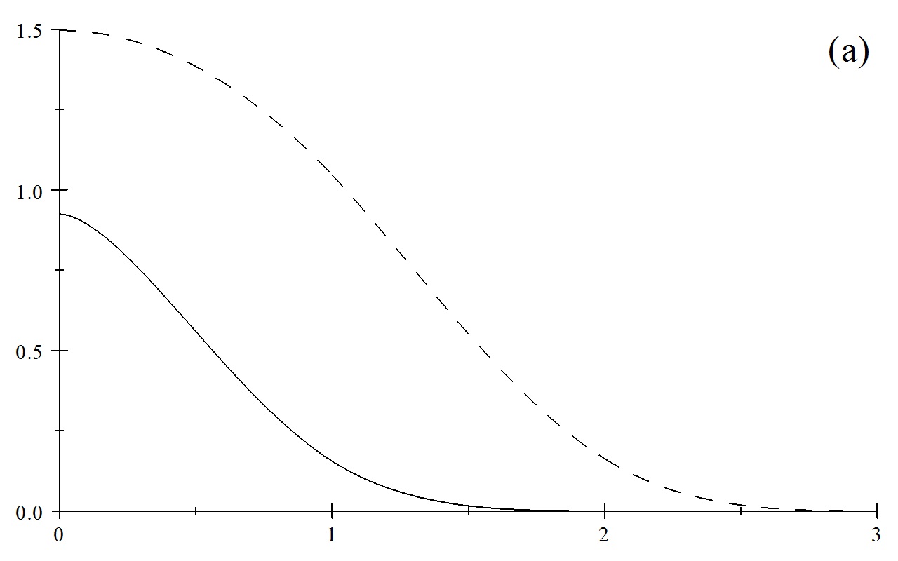
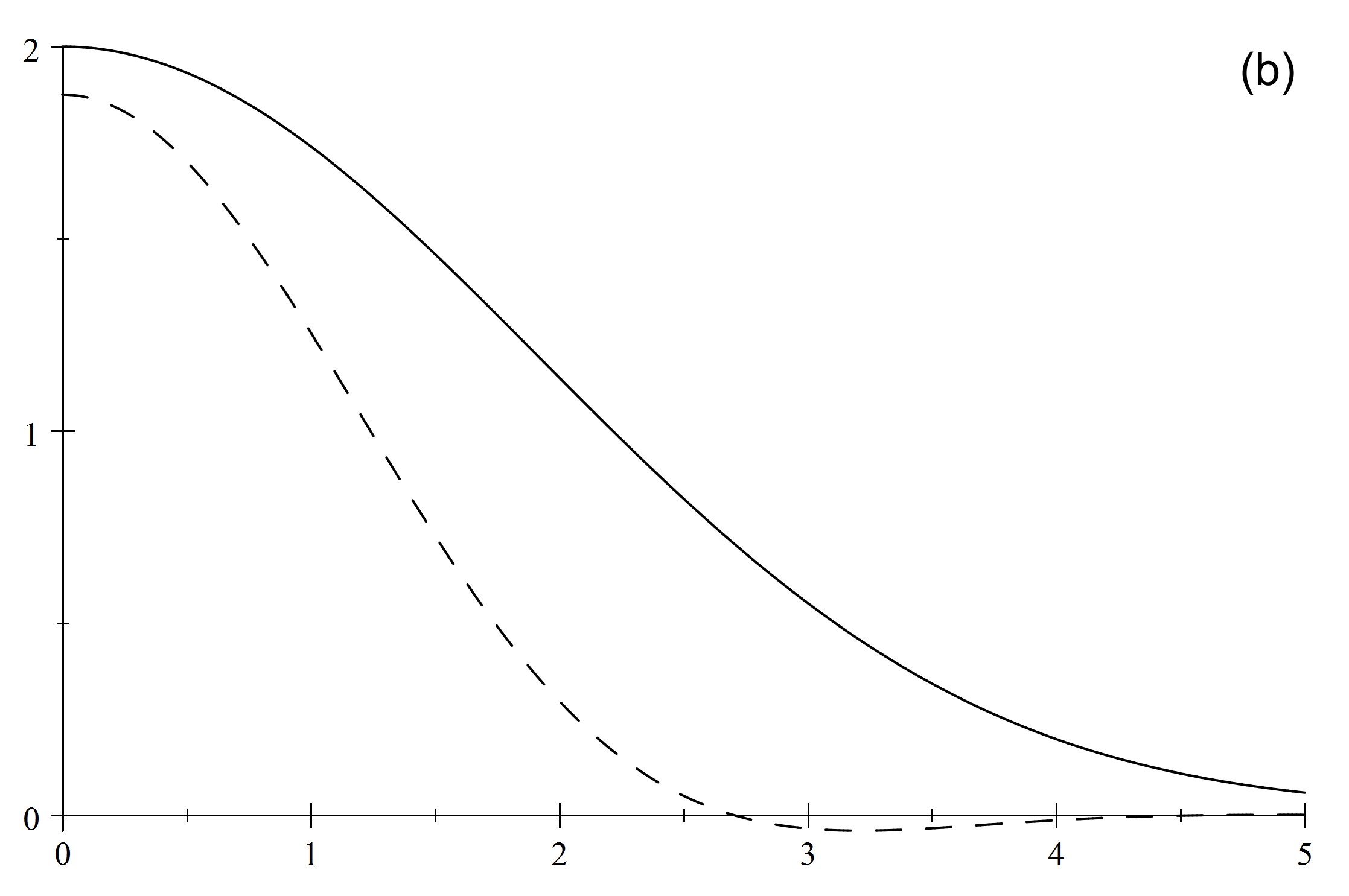
Although not revealed by their plots in Figure 2(a), there is a fundamental property that recommends against for use in RBF interpolation applications. Namely, if denotes the profile of the Fourier transform of the bivariate radially symmetric extension of , it is proved in [15] that satisfies a Sobolev regularity condition at . In particular, this implies for , hence is positive definite on . In contrast, using [15] to express in terms of the Bessel coefficient , it is verified numerically that takes both positive and negative values, as can be observed in Figure 2(b).
5.3 Examples of interpolatory -splines
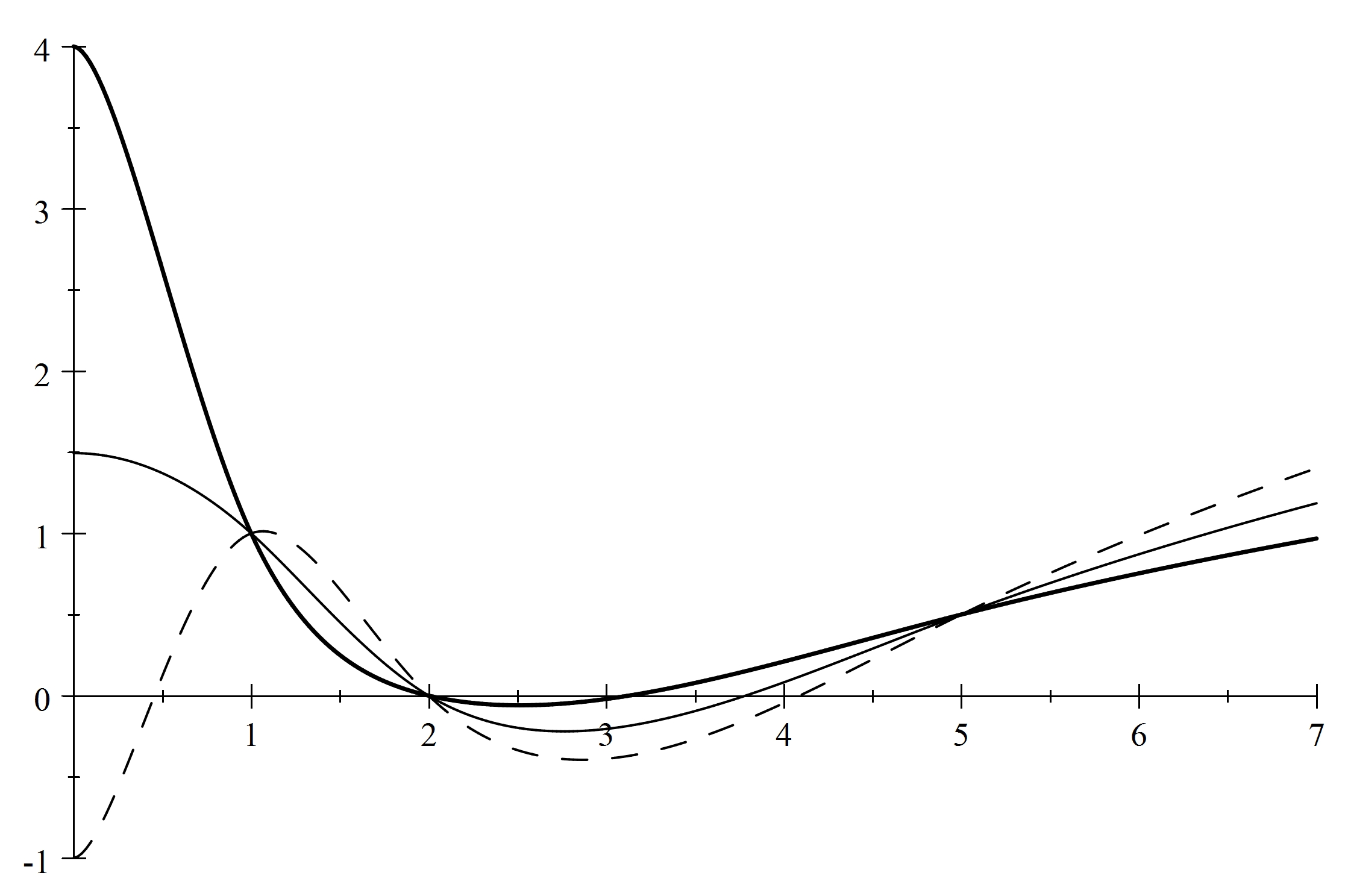
In this subsection, we illustrate some examples of Beppo Levi -splines that interpolate specific numerical data. Namely, we choose the cases of two knots in Figure 3 and three knots in Figure 4, with corresponding interpolation values , , . Note that this data is also used in Rabut’s numerical examples [21], except that in those examples has a value that is close to, but different from .

Using formula (22), our Beppo Levi -spline interpolants are expressed as
| (40) |
where in the case of only two knots. In each of the two figures, the thin line plot represents the non-singular interpolant of Theorem 2, whose coefficients satisfy the additional relation (23), i.e. , besides the interpolation conditions. The thick and dash line plots correspond to interpolants of the type of in Theorem 2, for which , a prescribed value.
Note that, in the case of two knots considered in Figure 3, there exists for which becomes a constant multiple of Johnson’s profile described in the previous subsection. This special value is used to generate the thick curve of Figure 3.
We remark that the thin line graphs of Figures 3 and 4 correspond to Rabut’s limit case in which and . In this case, Rabut’s observations [21, pp. 250–251] on the plot behaviour at and at can be explained, via our Proposition 1, by the form of the non-singular Beppo Levi -spline on the extreme subintervals.
6 Conclusion
We employed a -spline approach to the problem of minimizing the radial version (3) of the Beppo Levi energy integral over the full semi-axis , subject to interpolation conditions. This treatment led us to the identification of singular/non-singular solution profiles, which were expressed as linear combinations of dilates of a basis function. For and data functions from the radial energy space, our analysis proved the exact -approximation power of the -spline profiles. This result is further used in the sequel paper [8] to derive a -error bound for surface interpolation through curves prescribed on concentric circles.
Additional research is needed to establish the improved approximation order observed in our numerical experiments for data functions. Also, the close connections of Beppo Levi -splines with RBF and polyspline surfaces motivate the future extension of this work to higher order radially symmetric piecewise polyharmonic surfaces.
Acknowledgements. The author is grateful for the referees’ feedback, which has led to an improved presentation in the revised version.
References
- [1] J.H. Ahlberg, E.N. Nilson, J.L. Walsh, The Theory of Splines and Their Applications, Academic Press, New York, 1967.
- [2] R.S. Al-Sahli, -spline Interpolation and Biharmonic Polysplines on Annuli, MSc Thesis, Kuwait University (2012).
- [3] C. Arteaga, I. Marrero, A scheme for interpolation by Hankel translates of a basis function, J. Approx. Theory 164 (2012), 1540–1576.
- [4] A. Bejancu, Semi-cardinal polyspline interpolation with Beppo Levi boundary conditions, J. Approx. Theory 155 (2008), 52–73.
- [5] A. Bejancu, Transfinite thin plate spline interpolation, Constr. Approx. 34 (2011), 237–256.
- [6] A. Bejancu, Thin plate splines for transfinite interpolation at concentric circles, Math. Model. Anal. 18 (2013), 446–460.
- [7] A. Bejancu, Beppo Levi polyspline surfaces, in: The Mathematics of Surfaces XIV, R.J. Cripps, G. Mullineux, M.A. Sabin (Eds.), The Institute of Mathematics and its Applications, UK, 2013; ISBN 978-0-905091-30-3.
- [8] A. Bejancu, R.S. Al-Sahli, A new class of interpolatory -splines with adjoint end conditions, in: Curves and Surfaces 2014, J.-D. Boissonnat et al. (Eds.), LNCS 9213, Springer, 2015 (in press).
- [9] C. Bennett, R. Sharpley, Interpolation of Operators, Academic Press, Boston, 1988.
- [10] R. Cavoretto, G.E. Fasshauer, M.J. McCourt, An introduction to the Hilbert-Schmidt SVD using iterated Brownian bridge kernels, Numer. Algor. 68 (2015), 393–422.
- [11] J. Duchon, Interpolation des fonctions de deux variables suivant le principe de la flexion des plaques minces, RAIRO Anal. Numer. 10 (1976), 5–12.
- [12] R.L. Harder, R.N. Desmarais, Interpolation using surface splines, J. Aircraft 9 (1972), 189–191.
- [13] J. Jerome, J. Pierce, On spline functions determined by singular self-adjoint differential operators, J. Approx. Theory 5 (1972), 15–40.
- [14] M.J. Johnson, The -approximation order of surface spline interpolation for , Constr. Approx. 20 (2004), 303–324.
- [15] M.J. Johnson, Compactly supported, piecewise polyharmonic radial functions with prescribed regularity, Constr. Approx. 35 (2012), 201–223.
- [16] S. Karlin, Z. Ziegler, Tchebycheffian spline functions, SIAM J. Numer. Anal. 3 (1966), 514–543.
- [17] O.I. Kounchev, Minimizing the Laplacian of a function squared with prescribed values on interior boundaries—theory of polysplines, Trans. Am. Math. Soc. 350 (5) (1998), 2105–2128.
- [18] O.I. Kounchev, Multivariate Polysplines. Applications to Numerical and Wavelet Analysis, Academic Press, London, 2001.
- [19] E. Kreyszig, Introductory Functional Analysis with Applications, John Wiley & Sons, New York, 1978.
- [20] T.R. Lucas, A generalization of -splines, Numer. Math. 15 (1970), 359–370.
- [21] C. Rabut, Interpolation with radially symmetric thin plate splines, J. Comput. Appl. Math. 73 (1996), 241–256.
- [22] M.A. Sabin, Spline surfaces, Technical Report VTO/MS/156, Dynamics & Mathematical Services, British Aircraft Corporation Ltd., Weymouth, UK, 1969.
- [23] M.H. Schultz, R.S. Varga, -splines, Numer. Math. 10 (1967), 345–369.
- [24] L.L. Schumaker, Spline Functions: Basic Theory, third ed., Cambridge University Press, Cambridge, 2007.
- [25] J.P. Ward, M. Unser, Approximation properties of Sobolev splines and the construction of compactly supported equivalents, SIAM J. Math. Anal. 46 (2014), 1843–1858.
- [26] H. Wendland, Scattered Data Approximation. Cambridge University Press, Cambridge, 2005.