Scaling Algorithms for Weighted Matching in General Graphs

Abstract

We present a new scaling algorithm for maximum (or minimum) weight perfect matching on general, edge weighted graphs. Our algorithm runs in $O(m\sqrt{n}\log(nN))$ time, $O(m\sqrt{n})$ per scale, which matches the running time of the best cardinality matching algorithms on sparse graphs [36, 37, 20, 16]. Here $m,n,$ and $N$ bound the number of edges, vertices, and magnitude of any integer edge weight. Our result improves on a 25-year old algorithm of Gabow and Tarjan, which runs in $O(m\sqrt{n\log n\alpha(m,n)}\log(nN))$ time.

1 Introduction

In 1965 Edmonds [7, 8] proposed the complexity class $\mathbf{P}$ and proved that on general (non-bipartite) graphs, both the maximum cardinality matching and maximum weight matching problems could be solved in polynomial time. Subsequent work on general weighted graph matching focused on developing faster implementations of Edmonds’ algorithm [28, 12, 27, 21, 17, 14, 15] whereas others pursued alternative techniques such as cycle-canceling [3], weight-scaling [13, 20], or an algebraic approach using fast matrix multiplication [4]. Refer to Table 1 for a survey of weighted matching algorithms on general graphs. The fastest implementation of Edmonds’ algorithm [15] runs in $O(mn+n^{2}\log n)$ time on arbitrarily-weighted graphs. On graphs with integer edge-weights having magnitude at most $N$, Gabow and Tarjan’s [20] algorithm runs in $O(m\sqrt{n\alpha(m,n)\log n}\log(nN))$ time whereas Cygan, Gabow, and Sankowski’s runs in $O(Nn^{\omega})$ time with high probability, where $\omega$ is the matrix multiplication exponent. For reasonable values of $m,n,$ and $N$ the Gabow-Tarjan algorithm is theoretically superior to the others. However, it is an $\Omega(\sqrt{\log n\alpha(m,n)})$ factor slower than comparable algorithms for bipartite graphs [19, 30, 22, 6], and even slower than the interior point algorithm of [2] for sparse bipartite graphs. Moreover, its analysis is rather complex.

In this paper we present a new scaling algorithm for weighted matching on general graphs that runs in $O(m\sqrt{n}\log(nN))$ time. Each scale of our algorithm runs in $O(m\sqrt{n})$ time, which is asymptotically the same time required to compute a maximum cardinality matching in a sparse graph [36, 37, 20, 16]. Therefore, it is unlikely that our algorithm could be substantially improved without first finding a faster algorithm for the manifestly simpler problem of cardinality matching. Our algorithm’s time bound also matches that of the best bipartite scaling algorithms [19, 30, 22, 6], but is still slower than [2] on sufficiently sparse bipartite graphs.

Year Authors Time Complexity & Notes 1965 Edmonds $mn^{2}$    1974 Gabow    1976 Lawler $n^{3}$    1976 Karzanov $n^{3}+mn\log n$    1978 Cunningham & Marsh $\operatorname{poly}(n)$    1982 Galil, Micali & Gabow $mn\log n$    1985 Gabow $mn^{3/4}\log N$ integer weights    1989 Gabow, Galil & Spencer $mn\log\log\log_{d}n+n^{2}\log n$ $d=2+m/n$    1990 Gabow $mn+n^{2}\log n$    1991 Gabow & Tarjan $m\sqrt{n\alpha(n,m)\log n}\log(nN)$           integer weights    Cygan, Gabow    2012 & Sankowski $Nn^{\omega}$ randomized, integer weights    new $\operatorname{Edm}\cdot\sqrt{n}\log(nN)$ integer weights    $m\sqrt{n}\log(nN)$   

Table 1: Maximum Weight Perfect Matching (mwpm) algorithms for General Graphs. $\operatorname{Edm}$ is the time for one execution of Edmonds’ search on an integer-weighted graph.

1.1 Terminology

The input is a graph $G=(V,E,\hat{w})$ where $|V|=n,|E|=m$, and $\hat{w}:E\rightarrow\mathbb{R}$ assigns a real weight to each edge. A matching $M$ is a set of vertex-disjoint edges. A vertex is free if it is not adjacent to an $M$ edge. An alternating path is one whose edges alternate between $M$ and $E\setminus M$. An alternating path $P$ is augmenting if it begins and ends with free vertices, which implies that $M\oplus P\stackrel{{\scriptstyle\operatorname{def}}}{{=}}(M\cup P)\setminus(M\cap P)$ is also a matching and has one more edge. The maximum cardinality matching (mcm) problem is to find a matching $M$ maximizing $|M|$. The maximum weight perfect matching (mwpm) problem is to find a perfect matching $M$ (or, in general, one with maximum cardinality) maximizing $\hat{w}(M)=\sum_{e\in M}\hat{w}(e)$. The maximum weight matching problem (with no cardinality constraint) is reducible to mwpm [5] and may be a slightly easier problem [6, 25]. In this paper we assume that $\hat{w}:E\rightarrow\{0,\ldots,N\}$ assigns non-negative integer weights bounded by $N$.

1.2 Edmonds’ Algorithm

Edmonds’ mwpm algorithm begins with an empty matching $M$ and consists of a sequence of search steps, each of which performs zero or more dual adjustment, blossom shrinking, and blossom dissolution steps until a tight augmenting path emerges or the search detects that $|M|$ is maximum. (Blossoms, duals, and tightness are reviewed in Section 2.) The overall running time is therefore $O(n\cdot\operatorname{Edm})$, where $\operatorname{Edm}$ is the cost of one search. Gabow’s implementation [15] of Edmonds’ search runs in $O(m+n\log n)$ time, the same as one Hungarian search [10] on bipartite graphs.

1.3 Scaling Algorithms

The problem with Edmonds’ mwpm algorithm is that it finds augmenting paths one at a time, apparently dooming it to a running time of $\Omega(mn)$. The matching algorithms of [13, 20] take the scaling approach of Edmonds and Karp [9]. The idea is to expose the edge weights one bit at a time. In the $i$th scale the goal is to compute an optimum perfect matching with respect to the $i$ most significant bits of $\hat{w}$. Gabow [13] showed that each of $\log N$ scales can be solved in $O(mn^{3/4})$ time. Gabow and Tarjan [20] observed that it suffices to compute a $\pm O(n)$-approximate solution at each scale, provided there are additional scales; each of their $\log(nN)$ scales can be solved in $O(m\sqrt{n\alpha(m,n)\log n})$ time.

Scaling algorithms for general graph matching face a unique difficulty not encountered by scaling algorithms for other optimization problems. At the beginning of the $i$th scale we have inherited from the $(i-1)$th scale a nested set $\Omega^{\prime}$ of blossoms and near-optimal duals $y^{\prime},z^{\prime}$. (The matching primer in Section 2 reviews $y$ and $z$ duals.) Although $y^{\prime},z^{\prime}$ are numerically close to optimal, $\Omega^{\prime}$ may be structurally very far from optimal for scale $i$. The [13, 20] algorithms gradually get rid of inherited blossoms in $\Omega^{\prime}$ while simultaneously building up a new near-optimum solution $\Omega,y,z$. They decompose the tree of $\Omega^{\prime}$ blossoms into heavy paths and process the paths in a bottom-up fashion. Whereas Gabow’s method [13] is slow but moves the dual objective in the right direction, the Gabow-Tarjan method [20] is faster but may actually widen the gap between the dual objective and optimum. There are $\log n$ layers of heavy paths and processing each layer widens the gap by up to $O(n)$. Thus, at the final layer the gap is $O(n\log n)$. It is this gap that is the source of the $\sqrt{n\log n}$ factor in the running time of [20], not any data structuring issues.

Broadly speaking, our algorithm follows the scaling approach of [13, 20], but dismantles old blossoms in a completely new way, and further weakens the goal of each scale. Rather than compute an optimal [13] or near-optimal [20] perfect matching at each scale, we compute a near-optimal, near-perfect matching at each scale. The advantage of leaving some vertices unmatched (or, equivalently, artificially matching them up with dummy mates) is not at all obvious, but it helps speed up the dismantling of blossoms in the next scale. The algorithms are parameterized by a $\tau=\tau(n)$. A blossom is called large if it contains at least $\tau$ vertices and small otherwise. Each scale of our algorithm produces an imperfect matching $M$ with $y,z,\Omega$ that (i) leaves $O(n/\tau)$ vertices unmatched, and (ii) is such that the sum of $z(B)$ of all large $B\in\Omega$ is $O(n)$, independent of the magnitude of edge weights. After the last scale, the vertices left free by (i) will need to be matched up in $O(\operatorname{Edm}\cdot(n/\tau))$ time, at the cost of one Edmonds’ search per vertex. Thus, we want $\tau$ to be large. Part (ii) guarantees that large blossoms formed in one scale can be efficiently liquidated in the next scale (see Section 3), but getting rid of small blossoms (whose $z$-values are unbounded, as a function of $n$) is more complicated. Our methods for getting rid of small blossoms have running times that are increasing with $\tau$, so we want $\tau$ to be small. In the Liquidationist algorithm, all inherited small blossoms are processed in $O(\operatorname{Edm}\cdot\tau)$ time whereas in Hybrid (a hybrid of Liquidationist and Gabow’s algorithm [13]) they are processed in $O(m\tau^{3/4})$ time.

1.4 Organization

In Section 2 we review Edmonds’ LP formulation of mwpm and Edmonds’ search procedure. In Section 3 we present the Liquidationist algorithm running in $O(\operatorname{Edm}\cdot\sqrt{n}\log(nN))$ time. In Section 4 we give the Hybrid algorithm running in $O(m\sqrt{n}\log(nN))$ time.

Our algorithms depend on a having an efficient implementation of Edmonds’ search procedure. In Section 5 we give a detailed description of an implementation of Edmonds’ search that is very efficient on integer-weighted graphs. It runs in linear time when there are a linear number of dual adjustments. When the number of dual adjustments is unbounded it runs in $O(m\log\log n)$ time deterministically or $O(m\sqrt{\log\log n})$ time w.h.p. This implementation is based on ideas suggested by Gabow [13] and may be considered folklore in some quarters.

We conclude with some open problems in Section 6.

2 A Matching Primer

The mwpm problem can be expressed as an integer linear program

maximize $$\sum_{e\in E}x(e)\cdot\hat{w}(e)$$

subject to $$x(e)\in\{0,1\},\mbox{ for all $e\in E$}$$

and $$\sum_{e\ni v}x(e)=1,\mbox{ for all $v\in V$.}$$

The integrality constraint lets us interpret $\mathbf{x}$ as the membership vector of a set of edges and the $\sum_{e\ni v}x(e)=1$ constraint enforces that $\mathbf{x}$ represents a perfect matching. Birkhoff’s theorem [1] (see also von Neumann [38]) implies that in bipartite graphs the integrality constraint can be relaxed to $x(e)\in[0,1]$. The basic feasible solutions to the resulting LP correspond to perfect matchings. However, this is not true of non-bipartite graphs! Edmonds proposed exchanging the integrality constraint for an exponential number of the following odd set constraints, which are obviously satisfied for every $\mathbf{x}$ that is the membership vector of a matching.

$$\sum_{e\in E(B)}x(e)\leq\lfloor|B|/2\rfloor,\mbox{ for all $B\subset V$, $|B|\geq 3$ odd.}$$

Edmonds proved that the basic feasible solutions to the resulting LP are integral and therefore correspond to perfect matchings. Weighted matching algorithms work directly with the dual LP. Let $y:V\rightarrow\mathbb{R}$ and $z:2^{V}\rightarrow\mathbb{R}$ be the vertex duals and odd set duals.

minimize $$\sum_{v\in V}y(v)+\sum_{\begin{subarray}{c}B\subset V:\\ |B|\geq 3\,\operatorname{is}\,\operatorname{odd}\end{subarray}}z(B)\cdot\lfloor|B|/2\rfloor$$

subject to $$z(B)\geq 0,\mbox{ for all odd $B\subset V$,}$$

$$\hat{w}(u,v)\leq yz(u,v)\mbox{ for all $(u,v)\in E$,}$$

where, by definition, $$yz(u,v)\stackrel{{\scriptstyle\operatorname{def}}}{{=}}y(u)+y(v)+\sum_{B\supset\{u,v\}}z(B).$$

We generalize the synthetic dual $yz$ to an arbitrary set $S\subseteq V$ of vertices as follows.

$$yz(S)=\sum_{u\in S}y(u)\,+\,\sum_{B\subseteq S}z(B)\cdot\lfloor|B|/2\rfloor\,+\,\sum_{B\supset S}z(B)\cdot\lfloor|S|/2\rfloor.$$

Note that $yz(V)$ is exactly the dual objective.

Edmonds’ algorithm [7, 8] maintains a dynamic matching $M$ and dynamic laminar set $\Omega\subset 2^{V}$ of odd sets, each associated with a blossom subgraph. Informally, a blossom is an odd-length alternating cycle (w.r.t. $M$), whose constituents are either individual vertices or blossoms in their own right. More formally, blossoms are constructed inductively as follows. If $v\in V$ then the odd set $\{v\}$ induces a trivial blossom with edge set $\emptyset$. Suppose that for some odd $\ell\geq 3$, $A_{0},\ldots,A_{\ell-1}$ are disjoint sets associated with blossoms $E_{A_{0}},\ldots,E_{A_{\ell-1}}$. If there are edges $e_{0},\ldots,e_{\ell-1}\in E$ such that $e_{i}\in A_{i}\times A_{i+1}$ (modulo $\ell$) and $e_{i}\in M$ if and only if $i$ is odd, then $B=\bigcup_{i}A_{i}$ is an odd set associated with the blossom $E_{B}=\bigcup_{i}E_{A_{i}}\cup\{e_{0},\ldots,e_{\ell-1}\}$. Because $\ell$ is odd, the alternating cycle on $A_{0},\ldots,A_{\ell-1}$ has odd length, leaving $A_{0}$ incident to two unmatched edges, $e_{0}$ and $e_{\ell-1}$. One can easily prove by induction that $|B|$ is odd and that $E_{B}\cap M$ matches all but one vertex in $B$, called the base of $B$. Remember that $E(B)=E\cap{B\choose 2}$, the edge set induced by $B$, may contain many non-blossom edges not in $E_{B}$. Define $n(B)=|B|$ and $m(B)=|E(B)|$ to be the number of vertices and edges in the graph induced by $B$.

The set $\Omega$ of active blossoms is represented by rooted trees, where leaves represent vertices and internal nodes represent nontrivial blossoms. A root blossom is one not contained in any other blossom. The children of an internal node representing a blossom $B$ are ordered by the odd cycle that formed $B$, where the child containing the base of $B$ is ordered first. Edmonds [8, 7] showed that it is often possible to treat blossoms as if they were single vertices, by shrinking them. We obtain the shrunken graph $G/\Omega$ by contracting all root blossoms and removing the edges in those blossoms. To dissolve a root blossom $B$ means to delete its node in the blossom forest and, in the contracted graph, to replace $B$ with individual vertices $A_{0},\ldots,A_{\ell-1}$.

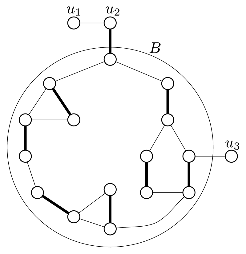
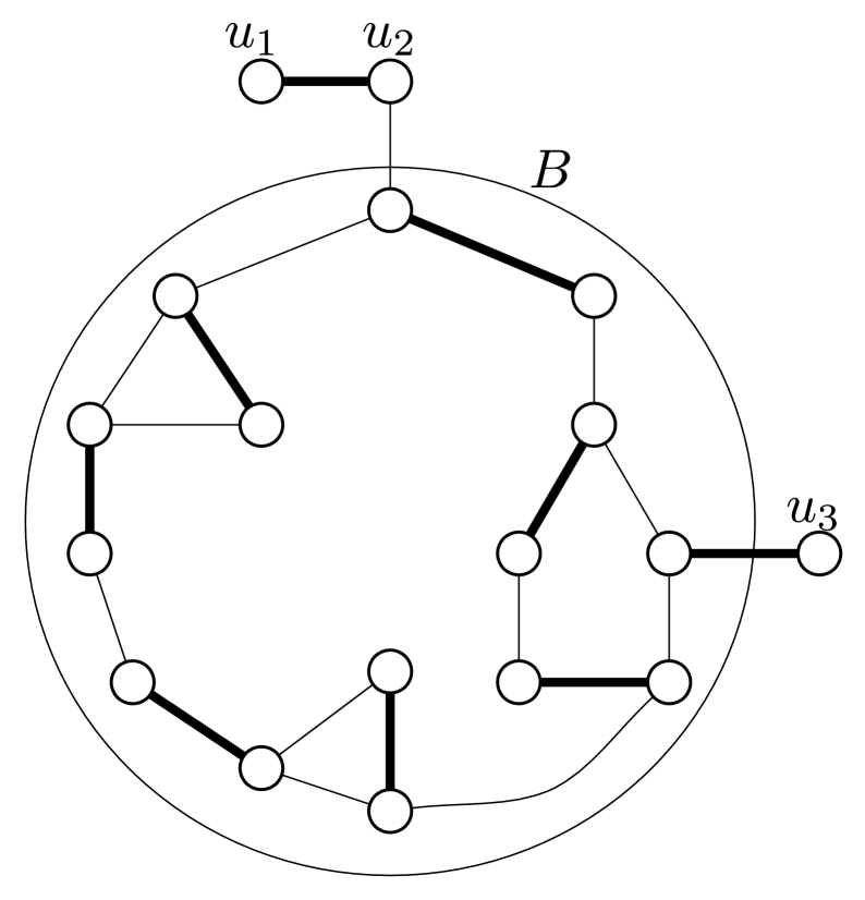
(a)	(b)

Figure 1: Matched edges are think, unmatched edges thin. Left: $B$ is a blossom consisting of 7 sub-blossoms, 4 of which are trivial (vertices) and the other three non-trivial blossoms. The path $P^{\prime}=(u_{1},u_{2},B,u_{3})$ is an augmenting path in the shrunken graph $G/\{B\}$. Right: augmenting along $P^{\prime}$ in $G/\{B\}$ enlarges the matching and has the effect of moving the base of $B$ to the vertex matched with $u_{3}$.

Blossoms have numerous properties. Our algorithms use two in particular.

1. The subgraph on $E_{B}$ is critical, meaning it contains a perfect matching on $B\backslash\{v\}$, for each $v\in B$. Phrased differently, any $v\in B$ can be made the base of $B$ by choosing the matching edges in $E_{B}$ appropriately.

2. As a consequence of (1), any augmenting path $P^{\prime}$ in $G/\Omega$ extends to an augmenting path $P$ in $G$, by replacing each non-trivial blossom vertex $B$ in $P^{\prime}$ with a corresponding path through $E_{B}$. Moreover, $\Omega$ is still valid for the matching $M\oplus P$, though the bases of blossoms intersecting $P$ may be relocated by augmenting along $P$. See Figure 1 for an example.

2.1 Relaxed Complementary Slackness

Edmonds’ algorithm maintains a matching $M$, a nested set $\Omega$ of blossoms, and duals $y:V\rightarrow\mathbb{Z}$ and $z:2^{V}\rightarrow\mathbb{N}$ that satisfy Property 1. Here $w$ is a weight function assigning even integers; it is generally not the same as the input weights $\hat{w}$.

Property 1.

(Complementary Slackness) Assume $w$ assigns only even integers.

1. Granularity. $z(B)$ is a nonnegative even integer and $y(u)$ is an integer.

2. Active Blossoms. $|M\cap E_{B}|=\lfloor|B|/2\rfloor$ for all $B\in\Omega$. If $B\in\Omega$ is a root blossom then $z(B)>0$; if $B\notin\Omega$ then $z(B)=0$. Non-root blossoms may have zero $z$-values.

3. Domination. $yz(e)\geq w(e)$, for each $e=(u,v)\in E$.

4. Tightness. $yz(e)=w(e)$, for each $e\in M\cup\bigcup_{B\in\Omega}E_{B}$.

Lemma 2.1.

If Property 1 is satisfied for a perfect matching $M$, blossom set $\Omega$, and duals $y,z$, then $M$ is necessarily a mwpm w.r.t. the weight function $w$.

The proof of Lemma 2.1 follows the same lines as Lemma 2.2, proved below. The Gabow-Tarjan algorithms and their successors [19, 20, 30, 22, 6, 5] maintain a relaxation of complementary slackness. By using Property 2 in lieu of Property 1 we introduce an additive error as large as $n$. This does not prevent us from computing exact mwpms but it does necessitate additional scales. Before the algorithm proper begins we compute the extended weight function $\bar{w}(e)=(\mbox{$\frac{n}{2}$}+1)\hat{w}(e)$. Note that the weight of every matching w.r.t. $\bar{w}$ is a multiple of $\mbox{$\frac{n}{2}$}+1$. After the final scale of our algorithms $w=2\bar{w}$ so if we can find a matching $M$ such that $w(M)$ is additively within $n$ of the mwpm, then $\bar{w}(M)$ is additively within $\frac{n}{2}$ of the mwpm, which implies that $M$ is exactly optimum w.r.t. both $\bar{w}(M)$ and $\hat{w}(M)$. These observations motivate the use of Property 2.

Property 2.

(Relaxed Complementary Slackness) Assume $w$ assigns only even integers. Property 1(1,2) holds and (3,4) are replaced with

1. Near Domination. $yz(e)\geq w(e)-2$ for each edge $e=(u,v)\in E$.

2. Near Tightness. $yz(e)\leq w(e)$, for each $e\in M\cup\bigcup_{B\in\Omega}E_{B}$.

The “-2” in Property 2 is due to the fact that $w$ is always even.

Lemma 2.2.

If Property 2 is satisfied for some perfect matching $M,$ blossom set $\Omega$, and duals $y,z$, then $w(M)\geq w(M^{*})-n$, where $M^{*}$ is an mwpm w.r.t. $w$.

Proof.

By Property 2 (near tightness and active blossoms), the definition of $yz$, and the perfection of $M$, we have

$$w(M) \geq\sum_{e\in M}yz(e)\>=\>\sum_{u\in V}y(u)+\sum_{B\in\Omega}z(B)\cdot|M\cap E(B)|\;\makebox[0.0pt][l]{$\displaystyle\>=\>\sum_{u\in V}y(u)+\sum_{B\in\Omega}z(B)\cdot\lfloor|B|/2\rfloor.$}$$

Since the mwpm $$M^{*} \lfloor|B|/2\rfloor B\in\Omega$$ puts at most edges in any blossom ,

$$w(M^{*}) \leq\sum_{e\in M^{*}}(yz(e)+2)$$ Property 2 (near domination)

$$=\sum_{u\in V}y(u)+\sum_{B\in\Omega}z(B)\cdot|M^{*}\cap E(B)|+2|M^{*}| yz$$ Defn. of

$$\leq\sum_{u\in V}y(u)+\sum_{B\in\Omega}z(B)\cdot\lfloor|B|/2\rfloor+n. |M^{*}|=n/2 z$$ , Non-negativity of

Therefore, we have $w(M)\geq w(M^{*})-n$. ∎

2.2 Edmonds’ Search

Suppose we have a matching $M$, blossom set $\Omega$, and duals $y,z$ satisfying Property 1 or 2. The goal of Edmonds’ search procedure is to manipulate $y,z,$ and $\Omega$ until an eligible augmenting path emerges. At this point $|M|$ can be increased by augmenting along such a path (or multiple such paths), which preserves Property 1 or 2. The definition of eligible needs to be compatible with the governing invariant (Property 1 or 2) and other needs of the algorithm. In our algorithms we use several implementations of Edmonds’ generic search: they differ in their governing invariants, definition of eligibility, and data structural details. For the time being the reader can imagine that Property 1 is in effect and that we use Edmonds’ original eligibility criterion [7].

Criterion 1.

An edge $e$ is eligible if it is tight, that is, $yz(e)=w(e)$.

Each scale of our algorithms begins with Property 1 as the governing invariant but switches to Property 2 when all inherited blossoms are gone. When Property 2 is in effect we use Criterion 2 if the algorithm aims to find augmenting paths in batches and Criterion 3 when augmenting paths are found one at a time. The reason for switching from Criterion 2 to 3 is discussed in more detail in the proof of Lemma 3.3.

Criterion 2.

An edge $e$ is eligible if at least one of the following holds.

1. $e\in E_{B}$ for some $B\in\Omega$.

2. $e\notin M$ and $yz(e)=w(e)-2$.

3. $e\in M$ and $yz(e)=w(e)$.

Criterion 3.

An edge is eligible if $yz(e)=w(e)$ or $yz(e)=w(e)-2$.

Regardless of which eligibility criterion is used, let $G_{\operatorname{elig}}=(V,E_{\operatorname{elig}})$ be the eligible subgraph and $\widehat{G}_{\operatorname{elig}}=G_{\operatorname{elig}}/\Omega$ be obtained from $G_{\operatorname{elig}}$ by contracting all root blossoms.

We consider a slight variant of Edmonds’ search that looks for augmenting paths only from a specified set $F$ of free vertices in $V$, that is, each augmenting path must have at least one end in $F$ and possibly both. (We also use $F$ to denote the corresponding free vertices in $\widehat{G}_{\operatorname{elig}}$.) The search iteratively performs Augmentation, Blossom Shrinking, Dual Adjustment, and Blossom Dissolution steps, halting after the first Augmentation step that discovers at least one augmenting path. We require that the $y$-values of all $F$ vertices have the same parity (even/odd). This is needed to keep $y,z$ integral and allow us to perform discrete dual adjustment steps without violating Property 1 or 2. See Figure 2 for the pseudocode.

$\mbox{\sc EdmondsSearch}(F)$           Precondition: $\{y(u)\;|\;u\in F\}$ must all be of the same parity. Repeatedly perform Augmentation, Blossom Shrinking, Dual Adjustment, and Blossom Dissolution steps. Halt after the first Augmentation step that finds at least one augmenting path. • Augmentation:
While $\widehat{G}_{\operatorname{elig}}$ contains an augmenting path from some free vertex in $F$, find such a path $\widehat{P}$ in $\widehat{G}_{\operatorname{elig}}$ and extend $\widehat{P}$ to an augmenting path $P$ in $G_{\operatorname{elig}}$. Set $M\leftarrow M\oplus P$ and update $\widehat{G}_{\operatorname{elig}}$. • Blossom Shrinking:
Let $\widehat{V}_{\operatorname{out}}\subseteq V(\widehat{G}_{\operatorname{elig}})$ be the vertices (that is, root blossoms) reachable from free vertices in $F$ by even-length alternating paths in $\widehat{G}_{\operatorname{elig}}$; let $\Omega_{\operatorname{new}}$ be a maximal set of (nested) blossoms on $\widehat{V}_{\operatorname{out}}$ (That is, if $(u,v)\in E(\widehat{G}_{\operatorname{elig}})\backslash M$ and $u,v\in\widehat{V}_{\operatorname{out}}$, then $u$ and $v$ must be in a common blossom in $\Omega_{\operatorname{new}}$.) Let $\widehat{V}_{\operatorname{in}}\subseteq V(\widehat{G}_{\operatorname{elig}})\backslash\widehat{V}_{\operatorname{out}}$ be those vertices reachable from free vertices in $F$ by odd-length alternating paths. Set $z(B)\leftarrow 0$ for $B\in\Omega_{\operatorname{new}}$ and set $\Omega\leftarrow\Omega\cup\Omega_{\operatorname{new}}$. Update $\widehat{G}_{\operatorname{elig}}$. • Dual Adjustment:
Let $V_{\operatorname{in}},V_{\operatorname{out}}\subseteq V$ be original vertices represented by vertices in $\widehat{V}_{\operatorname{in}}$ and $\widehat{V}_{\operatorname{out}}$. The $y$- and $z$-values for some vertices and root blossoms are adjusted: $\displaystyle y(u)$ $\displaystyle\leftarrow y(u)-1,\mbox{ for all $u\in V_{\operatorname{out}}$.}$ $\displaystyle y(u)$ $\displaystyle\leftarrow y(u)+1,\mbox{ for all $u\in V_{\operatorname{in}}$.}$ $\displaystyle z(B)$ $\displaystyle\leftarrow z(B)+2,\mbox{ if $B\in\Omega$ is a root blossom with $B\subseteq V_{\operatorname{out}}$.}$ $\displaystyle z(B)$ $\displaystyle\leftarrow z(B)-2,\mbox{ if $B\in\Omega$ is a root blossom with $B\subseteq V_{\operatorname{in}}$.}\hskip 142.26378pt$ • Blossom Dissolution:
After dual adjustments some (inner) root blossoms may now have zero $z$-values. Repeatedly dissolve such blossoms (remove them from $\Omega$) as long as they exist. Update $\widehat{G}_{\operatorname{elig}}$.

Figure 2: A generic implementation of Edmonds’ search procedure. Data structural issues are ignored, as is the eligibility criterion, which determines $\widehat{G}_{\operatorname{elig}}$.

The main data structure needed to implement EdmondsSearch is a priority queue for scheduling events (blossom dissolution, blossom formation, and grow events that add vertices to $V_{\operatorname{in}}\cup V_{\operatorname{out}}$). We refer to PQSearch as an implementation of EdmondsSearch when the number of dual adjustments is unbounded. See Gabow [15] for an implementation of PQSearch taking $O(m+n\log n)$ time, or Section 5 for one taking $O(m\sqrt{\log\log n})$ time, w.h.p. When the number of dual adjustments is $t=O(m)$ we can use a trivial array of buckets as a priority queue. Let BucketSearch be an implementation of EdmondsSearch running in $O(m+t)$ time; refer to Section 5 for a detailed description.

Regardless of what $t$ is or how the dual adjustments are handled, we still have options for how to implement the Augmentation step. Under Criterion 1 of eligibility, we can make the Augmentation step extend $M$ to a maximum cardinality matching in the subgraph of $G_{\operatorname{elig}}$ induced by $V(M)\cup F$. This can be done in $O((p+1)m)$ time if $p\geq 0$ augmenting paths are found [18], or in $O(m\sqrt{n})$ time, independent of $p$, using a cardinality matching algorithm, e.g., [29, 36, 37] or [20, §10] or [16].

When eligibility Criterion 2 is in effect the Augmentation step is qualitatively different. Observe that in the contracted graph $G/\Omega$, matched and unmatched edges have different eligibility criteria. It is easily proved that augmenting along a maximal set of augmenting paths eliminates all eligible augmenting paths, quickly paving the way for Blossom Shrinking and Dual Adjustment steps. Unlike PQSearch and BucketSearch, SearchOne only performs one dual adjustment and must be used with Criterion 2. Finding a maximal set of augmenting paths in $O(m)$ time is straightforward with depth first search [20, §8] and a union-find algorithm [18].

$\mbox{\sc SearchOne}(F)$          Precondition: $\{y(u)\;|\;u\in F\}$ must all be of the same parity. • Augmentation:
Find a maximal set $\Psi$ of vertex-disjoint augmenting paths from $F$ in $\widehat{G}_{\operatorname{elig}}$. Set $\displaystyle M\leftarrow M\oplus\bigcup_{P\in\Psi}P$. • Perform Blossom Shrinking, Dual Adjustment, and Blossom Dissolution steps from $F$, exactly as in EdmondsSearch.

Figure 3:

The following lemmas establish the correctness of EdmondsSearch (using either Property 1 or 2) and SearchOne (using Property 2 and Criterion 2).

Lemma 2.3.

After the Augmentation step of $\mbox{\sc SearchOne}(F)$ (using Criterion 2 for eligibility), $\widehat{G}_{\operatorname{elig}}$ contains no eligible augmenting paths from an $F$-vertex.

Proof.

Suppose that, after the Augmentation step, there is an augmenting path $P$ from an $F$-vertex in $\widehat{G}_{\operatorname{elig}}$. Since $\Psi$ was maximal, $P$ must intersect some $P^{\prime}\in\Psi$ at a vertex $v$. However, after the Augmentation step every edge in $P^{\prime}$ will become ineligible, so the matching edge $(v,v^{\prime})\in M$ is no longer in $\widehat{G}_{\operatorname{elig}}$, contradicting the fact that $P$ consists of eligible edges. ∎

Lemma 2.4.

If Property 1 is satisfied and the $y$-values of vertices in $F$ have the same parity, then $\mbox{\sc EdmondsSearch}(F)$ (under Criterion 1) preserves Property 1.

Proof.

Property 1 (granularity) is obviously maintained, since we are always adjusting $y$-values by 1 and $z$-values by 2. Property 1 (active blossoms) is also maintained since all the new root blossoms discovered in the Blossom Shrinking step are in $V_{\operatorname{out}}$ and will have positive $z$-values after adjustment. Furthermore, each root blossom whose $z$-value drops to zero is removed.

Consider the tightness and the domination conditions of Property 1. First note that if both endpoints of $e$ lie in the same blossom, $yz(e)$ will not change until the blossom is dissolved. When the blossom was formed, the blossom edges must be eligible (tight). The augmentation step only makes eligible edges matched, so tightness is satisfied.

Consider the effect of a dual adjustment on an edge $e=(u,v)$, whose endpoints lie in different blossoms. We divide the analysis into the following four cases. Refer to Figure 4 for illustrations of the cases.

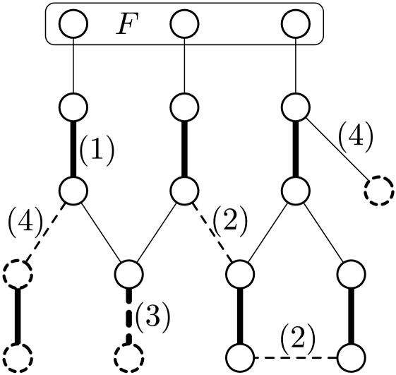
Figure 4: Thick edges are matched, thin unmatched. Dashed edges (whether thick or thin) are ineligible. Solid vertices are in $V_{\operatorname{in}}\cup V_{\operatorname{out}}$; all other vertices are dashed. Case (3) can only occur under Criteria 2 or 3 of eligibility.

1. Both $u$ and $v$ are in $V_{\operatorname{in}}\cup V_{\operatorname{out}}$ and $e\in M$. We cannot have both $u,v\in V_{\operatorname{out}}$ (otherwise they would be in a common blossom, since $e$ is eligible) nor can both be in $V_{\operatorname{in}}$, so $u\in V_{\operatorname{in}},v\in V_{\operatorname{out}}$ and $yz(e)$ is unchanged.

2. Both $u$ and $v$ are in $V_{\operatorname{in}}\cup V_{\operatorname{out}}$ and $e\notin M$. If at least one of $u$ or $v$ is in $V_{\operatorname{in}}$, then $yz(e)$ cannot decrease and domination holds. Otherwise we must have $u,v\in V_{\operatorname{out}}$. In this case, $e$ must be ineligible, for otherwise an augmenting path or a blossom would have been found. Ineligibility implies $yz(e)\geq w(e)+1$ but something stronger can be inferred. Since the $y$-values of free vertices have the same parity, all vertices reachable from free vertices by eligible alternating paths also have the same parity. Since $w(e)$ is even (by assumption) and $yz(e)$ is even (by parity) we can conclude that $yz(e)\geq w(e)+2$ before dual adjustment, and therefore $yz(e)\geq w(e)$ after dual adjustment.

3. $u$ but not $v$ is in $V_{\operatorname{in}}\cup V_{\operatorname{out}}$ and $e\in M$. This case cannot happen since in this case, $u\in V_{\operatorname{in}}$ and $e$ must be ineligible, but we know all matched edges are tight.

4. $u$ but not $v$ is in $V_{\operatorname{in}}\cup V_{\operatorname{out}}$ and $e\notin M$. If $u\in V_{\operatorname{in}}$, then $yz(e)$ increases and domination holds. Otherwise, $u\in V_{\operatorname{out}}$ and $e$ must be ineligible. In this case, we have $yz(e)\geq w(e)+1$ before the dual adjustment and $yz(e)\geq w(e)$ afterwards.

∎

Lemma 2.5.

If Property 2 is satisfied and the $y$-values of vertices in $F$ have the same parity, then $\mbox{\sc SearchOne}(F)$ (under Criterion 2) or $\mbox{\sc EdmondsSearch}(F)$ (under Criterion 3) preserves Property 2.

Proof.

The proof is similar to that of the previous lemma, except that we replace the tightness and domination by near tightness and near domination. We point out the differences in the following. An edge $e$ can be included in a blossom only if it is eligible. An eligible edge must have $yz(e)=w(e)$ or $yz(e)=w(e)-2$. Augmentations only make eligible edges matched. Therefore near tightness is satisfied after the Augmentation step.

When doing the dual adjustment, the following are the cases when $yz(e)$ is modified after the dual adjustment. In Case 2 of the previous proof, when $u,v\in V_{\operatorname{out}}$ but $e$ is ineligible we have $yz(e)\geq w(e)-1$. By parity this implies that $yz(e)\geq w(e)$ before the dual adjustment and $yz(e)\geq w(e)-2$ afterwards. Case 3 may happen in this situation. It is possible that $u\in V_{\operatorname{in}}$ and $e\in M$ is ineligible. Then we must have $yz(e)\leq w(e)-1$ before the dual adjustment and $yz(e)\leq w(e)$ afterwards. In Case 4, when $u\in V_{\operatorname{out}}$, we have $yz(e)\geq w(e)-1$ before the dual adjustment and $yz(e)\geq w(e)-2$ afterwards. ∎

3 The Liquidationist Algorithm

The most expedient way to get rid of an inherited blossom is to liquidate it (our term) by distributing its $z$-value over its constituents’ $y$-values, preserving Property 1 (domination).

Liquidate($B$) : $y(u)\leftarrow y(u)+z(B)/2$  for all $u\in B$ $z(B)\leftarrow 0$   (and dissolve $B$)

From the perspective of a single edge, liquidation has no effect on $yz(e)$ if $e$ is fully inside $B$ or outside $B$, but it increases $yz(e)$ by $z(B)/2$ if $e$ straddles $B$. From a global perspective, liquidation increases the dual objective $yz(V)$ by $|B|\cdot z(B)/2-\lfloor|B|/2\rfloor\cdot z(B)=z(B)/2$. Since $z(B)$ is generally unbounded (as a function of $n$), this apparently destroys the key advantage of scaling algorithms, that $yz(V)$ is within $O(n)$ of optimum. It is for this reason that [13, 20] did not pursue liquidation.

The Liquidationist algorithm (see Figure 5) is so named because it liquidates all inherited blossoms. Let $w^{\prime},y^{\prime},z^{\prime},M^{\prime},\Omega^{\prime}$ be the edge weights, dual variables, matching and blossom set at the end of the $(i-1)$th scale. Recall that a blossom is large if it contains at least $\tau$ vertices and small otherwise.

The first step is to compute the even weight function $w$ for the $i$th scale and starting duals $y,z$, as follows.

$$w(e) \leftarrow 2(w^{\prime}(e)+\mbox{the $i$th bit of $\bar{w}(e)$}),$$

$$y(u) \leftarrow 2y^{\prime}(u)+3,$$

$$z(B) \leftarrow 2z^{\prime}(B).$$

Lemma 3.1 proves that if $w^{\prime},y^{\prime},z^{\prime}$ satisfy Property 2 w.r.t. $M^{\prime}$, then $w,y,z$ satisfy Property 1 w.r.t. $M=\emptyset$, except for the Active Blossom property, a point that will be moot once we liquidate all blossoms in $\Omega^{\prime}$. It will be guaranteed that $\sum_{\operatorname{Large}\,B\in\Omega^{\prime}}z(B)=O(n)$, so liquidating all large blossoms increases $yz(V)$ by a tolerable $O(n)$. After liquidating large blossoms, but before liquidating small blossoms, we reweight the graph, setting

$$w(u,v) \leftarrow w(u,v)-y(u)-y(v) (u,v)$$ for each edge

$$y(u) \leftarrow 0 u$$ for each vertex

Reweighting is a conceptual trick that simplifies the presentation and some proofs. A practical implementation would simulate this step without actually modifying the edge weights.

Liquidating small blossoms increases $y(u)$ from 0 to $\sum_{\operatorname{Small}\,B\in\Omega^{\prime},\,u\in B}z(B)/2$, which temporarily destroys the property that $yz(V)$ is within $O(n)$ of optimal. Let $B^{\prime}$ be a maximal former small blossom. We repeatedly execute $\mbox{\sc PQSearch}(F)$ from the set $F$ of free vertices in $B^{\prime}$ with maximum $y$-value $Y$ until one of three events occurs (i) $|F|$ decreases, because an augmenting path is discovered, (ii) $|F|$ increases because $Y-Y^{\prime}$ dual adjustments have been performed, where $Y^{\prime}$ is the 2nd largest $y$-value of a free vertex in $B^{\prime}$, or (iii) the $y$-values of all vertices in $F$ become zero. Because $B^{\prime}$ is small there can be at most $O(|B^{\prime}|)=O(\tau)$ executions that stop due to (i) and (ii). We prove that conducting Edmonds’ searches in exactly this way has two useful properties. First, no edge straddling $B^{\prime}$ ever becomes eligible, so the search is confined to the subgraph induced by $B^{\prime}$, and second, when the $y$-values of free vertices are zero, $yz(V)$ is restored to be within $O(n)$ of optimal. Each of these Edmonds’ searches can form new weighted blossoms, but because of the first property they all must be small. The second property is essential for the next step: efficiently finding a near-perfect matching.

After inherited blossoms have been dealt with, we switch from satisfying Property 1 to Property 2 and call $\mbox{\sc SearchOne}(F)$ $\tau$ times using eligibility Criterion 2, where $F$ is the set of all free vertices. We prove that this leaves at most $O(n/\tau)$ free vertices. Note that large blossoms can only be introduced during the calls to SearchOne. Since we only perform $\tau$ dual adjustments, we can bound the sum of $z$-values of all new large blossoms by $O(n)$.

To end the $i$th scale we artificially match up all free vertices with dummy vertices and zero-weight edges, yielding a perfect matching. Thus, the input graph $G_{i+1}$ to scale $i+1$ is always $G$ supplemented with some dummy pendants (degree one vertices) that have accrued over scales 1 through $i$. Pendants can never appear in a blossom.

After the last scale, we have a perfect matching $M$ in $G_{\lceil\log((\frac{n}{2}+1)N)\rceil}$, which includes up to $O(n/\tau)\cdot\log((\frac{n}{2}+1)N)$ dummy vertices acquired over all the scales. We delete all dummy vertices and repeatedly call $\mbox{\sc PQSearch}(F)$ on the current set of free vertices until $F=\emptyset$. Since these calls make many dual adjustments, we switch from Criterion 2 (which is only suitable for use with SearchOne) to Criterion 3 of eligibility. Each call to PQSearch matches at least two vertices so the total time for finalization is $O(\operatorname{Edm}\cdot(n/\tau)\log(nN))$. See Figure 5 for a compact summary of the whole algorithm.

$\mbox{\sc Liquidationist}(G,\hat{w})$ • $G_{0}\leftarrow G,y\leftarrow 0,z\leftarrow 0,w\leftarrow 0$, $\Omega\leftarrow\emptyset$. • For scales $i=1,\cdots,\lceil\log((\frac{n}{2}+1)N)\rceil$, execute steps Initialization–Perfection. Initialization 1. Set $G_{i}\leftarrow G_{i-1}$, $y^{\prime}\leftarrow y$, $z^{\prime}\leftarrow z$, $w^{\prime}\leftarrow w$, $M\leftarrow\emptyset$, $\Omega^{\prime}\leftarrow\Omega$, and $\Omega\leftarrow\emptyset$. Scaling 2. Set $w(e)\leftarrow 2(w^{\prime}(e)+\mbox{(the $i^{\operatorname{th}}$ bit of $\bar{w}(e)$)})$ for each edge $e$, set $y(u)\leftarrow 2y^{\prime}(u)+3$ for each vertex $u$, and $z(B^{\prime})\leftarrow 2z^{\prime}(B^{\prime})$ for each $B^{\prime}\in\Omega^{\prime}$. Large Blossom Liquidation and Reweighting 3. $\mbox{\sc Liquidate}(B^{\prime})$ for each large $B^{\prime}\in\Omega^{\prime}$. 4. Reweight the graph: $\displaystyle w(u,v)$ $\displaystyle\leftarrow w(u,v)-y(u)-y(v)$ for each edge $(u,v)\in E$ $\displaystyle y(u)$ $\displaystyle\leftarrow 0$ for each vertex $u\in V$ Small Blossom Liquidation 5. $\mbox{\sc Liquidate}(B^{\prime})$ for each small $B^{\prime}\in\Omega^{\prime}$. 6. For each maximal old small blossom $B^{\prime}$:
      While $\max\{y(u)\;|\;u\in B^{\prime}\mbox{ is free}\}>0$, $\displaystyle Y$ $\displaystyle\leftarrow\max\{y(u)\,|\,u\in B^{\prime}\mbox{ is free}\}$ $\displaystyle F$ $\displaystyle\leftarrow\{u\in B^{\prime}\mbox{ is free}\,|\,y(u)=Y\}$ $\displaystyle Y^{\prime}$ $\displaystyle\leftarrow\max\{0,\max\{y(u)\,|\,u\in B^{\prime}\backslash F\mbox{ is free}\}\}\hskip 110.96556pt$ Run $\mbox{\sc PQSearch}(F)$ (Criterion 1) until an augmenting path is found and
            the matching is augmented or $Y-Y^{\prime}$ dual adjustments have been performed.
Free Vertex Reduction 7. Run $\mbox{\sc SearchOne}(F)$ (Criterion 2) $\tau$ times, where $F$ is the set of free vertices. Perfection 8. Delete all free dummy vertices. For each remaining free vertex $u$, create a dummy $\hat{u}$ with $y(\hat{u})=\tau$ and a zero-weight matched edge $(u,\hat{u})\in M$.
• Finalization
Delete all dummy vertices from $G_{\lceil\log((\frac{n}{2}+1)N)\rceil}$. Repeatedly call $\mbox{\sc PQSearch}(F)$ (Criterion 3) on the set $F$ of free vertices until $F=\emptyset$.

Figure 5:

3.1 Correctness

We first show that rescaling $w,y,z$ at the beginning of a scale restores Property 1 (except for Active Blossoms) assuming Property 2 held at the end of the previous scale.

Lemma 3.1.

Consider an edge $e\in E(G_{i})$ at scale $i$.

• After Step 2 (Scaling), $w(e)\leq yz(e)$. Moreover, if $e\in M^{\prime}\cup\bigcup_{B^{\prime}\in\Omega^{\prime}}E_{B^{\prime}}$ then $w(e)\geq yz(e)-6$. (In the first scale, $w(e)\geq yz(e)-6$ for every $e$.)

• After Step 4 (Large Blossom Liquidation and Reweighting), $w(e)$ is even for all $e\in E(G_{i})$ and $y(u)=0$ for all $y\in V(G_{i})$. Furthermore,

  $$w(e)\leq yz(e)=\sum_{\begin{subarray}{c}\operatorname{Small}\,B^{\prime}\in\Omega^{\prime}\;:\\ e\in E(B^{\prime})\end{subarray}}z(B^{\prime}).$$

Therefore, after Large Blossom Liquidation and Reweighting, $(M,\Omega,y,z,w)$ satisfy Property 1, excluding Active Blossoms.

Proof.

At the end of the previous scale, by Property 2(near domination), $y^{\prime}z^{\prime}(e)\geq w^{\prime}(e)-2$. After the Scaling step,

$$yz(e)=2y^{\prime}z^{\prime}(e)+6\geq 2w^{\prime}(e)+2\geq w(e).$$

If $e\in M^{\prime}\cup\bigcup_{B^{\prime}\in\Omega^{\prime}}E_{B^{\prime}}$ was an old matching or blossom edge then

$$yz(e)=2y^{\prime}z^{\prime}(e)+6\leq 2w^{\prime}(e)+6\leq w(e)+6.$$

In the first scale, $yz(e)=6$ and $w(e)\in\{0,2\}$. Step 3 will increase some $yz$-values and $w(e)\leq yz(e)$ will be maintained. After Step 4 (reweighting), $w(u,v)$ will be reduced by $y(u)+y(v)$, so

$$w(u,v)\leq\sum_{\begin{subarray}{c}\operatorname{Small}\,B^{\prime}\in\Omega^{\prime}:\\ (u,v)\in E(B^{\prime})\end{subarray}}z(B^{\prime}).$$

From Property 2(1) (granularity) in the previous scale, after Step 2 all $y$-values are odd and $z$-values are multiples of 4. Therefore $y$-values remain odd after Step 3. Since $w(u,v)$ is even initially, it remains even after subtracting off odd $y(u),y(v)$ in Step 4. ∎

Lemma 3.2.

After Step 5 in Small Blossom Liquidation, we have $w(u,v)\leq 2\cdot\min\{y(u),y(v)\}$ for all edges $(u,v)$, hence, $w(u,v)\leq y(u)+y(v)$. Furthermore, Property 1 holds after Small Blossom Liquidation.

Proof.

Fix any edge $(u,v)$. According to Lemma 3.1, after Step 5 we have

$$y(u)=\sum_{\begin{subarray}{c}\operatorname{Small}\,B^{\prime}\in\Omega^{\prime}:\\ u\in B^{\prime}\end{subarray}}z(B^{\prime})/2\;\geq\;\sum_{\begin{subarray}{c}\operatorname{Small}\,B^{\prime}\in\Omega^{\prime}:\\ (u,v)\in E(B^{\prime})\end{subarray}}z(B^{\prime})/2\;\geq\;w(u,v)/2.$$

Therefore, $w(u,v)\leq 2y(u)$ and by symmetry, $w(u,v)\leq 2y(v)$. After Step 5, $z=0$ and $\Omega=\emptyset$, so Property 1 (including Active Blossoms) holds. In Step 6 of Small Blossom Liquidation, PQSearch is always searching from the free vertices with the same $y$-values and the edge weights are even. Therefore, by Lemma 2.4, Property 1 holds afterwards. ∎

Lemma 3.3.

The Liquidationist algorithm returns a maximum weight perfect matching of $G$.

Proof.

First we claim that at the end of each scale $i$, $M$ is a perfect matching in $G_{i}$ and Property 2 is satisfied. By Lemma 3.2, Property 1 is satisfied after the Small Blossom Liquidation step. The calls to SearchOne in the Free Vertex Reduction step always search from free vertices with the same $y$-values. Therefore, by Lemma 2.5, Property 2 holds afterwards. The perfection step adds/deletes dummy free vertices and edges to make the matching $M$ perfect. The newly added edges have $w(e)=yz(e)$, and so Property 2 is maintained at the end of scale $i$.

Therefore, Property 2 is satisfied at the end of the last scale $\lceil\log((\mbox{$\frac{n}{2}$}+1)N)\rceil$. Consider the shrunken blossom edges at this point in the algorithm. Each edge $e$ was made a blossom edge when it was eligible according to Criterion 1 (in Step 6) or Criterion 2 (in Step 7) and may have participated in augmenting paths while its blossom was still shrunken. Thus, all we can claim is that $yz(e)-w(e)\in\{0,-2\}$. In the calls to PQSearch in the Finalization step we switch to eligibility Criterion 3 in order to ensure that edges inside shrunken blossoms remain eligible whenever the blossoms are dissolved in the course of the search. By Lemma 2.5, each call to PQSearch maintains Property 2 while making the matching perfect. After Finalization, $w(M)\geq w(M^{*})-n$. Note that in the last scale ${w}(e)=2\bar{w}(e)$ for each edge $e$, so $\bar{w}(M)\geq\bar{w}(M^{*})-n/2$. By definition of $\bar{w}$, $\bar{w}(M)$ is a multiple of $\mbox{$\frac{n}{2}$}+1$, so $M$ maximizes $\bar{w}(M)$ and hence $\hat{w}(M)$ as well. ∎

3.2 Running time

Next, we analyze the running time.

Lemma 3.4.

In Step 6, we only need to consider the edges within small blossoms of the previous scale. The total time needed for Step 6 in one scale is $O((m+n\log n)\tau)$ (using [15]) or $O(m\sqrt{\log\log n}\cdot\tau)$ w.h.p. (see Section 5).

Proof.

We first analyze the behavior of Step 6 assuming we only consider edges with both endpoints in the same maximal small blossom, i.e., straddling edges are ignored. Then we argue that straddling edges can never become eligible in Step 6, so a correct implementation may ignore them.

Let $Y$ denote the current maximum $y$-value of a free vertex in a maximal small blossom $B$ processed in Step 6. We prove by induction that the $y$-values of all vertices in $V_{\operatorname{in}}\cup V_{\operatorname{out}}$ are at least $Y$. The proof is by induction. After Initialization, since $M=\emptyset$, we have $V_{\operatorname{in}}\cup V_{\operatorname{out}}=F$. Suppose that it is true before a dual adjustment in $\mbox{\sc PQSearch}(F)$. After the dual adjustment, the maximum $y$-value of a free vertex is now $Y-1$. Vertices can have their $y$-values decreased by at most one which may cause new edges straddling $V_{\operatorname{in}}\cup V_{\operatorname{out}}$ to become eligible. Suppose that $(u,v)\in E(B)$ becomes eligible after the dual adjustment, adding $v\in B$ to the set $V_{\operatorname{in}}\cup V_{\operatorname{out}}$. The eligibility criterion is tightness (Criterion 1), so we must have $w(u,v)=y(u)+y(v)\geq(Y-1)+y(v)$. On the other hand, by Lemma 3.2 and since $y(v)$ has not been changed since Step 5, we have $w(u,v)\leq 2y(v)$. Therefore, $y(v)\geq Y-1$.

Now consider an edge $(u,v)$ with $u$ and $v$ in different maximal small blossoms. Just before we liquidate small blossoms, $w(u,v)\leq yz(u,v)=y(u)+y(v)=0$; after liquidation we have $yz(u,v)=Y_{u}+Y_{v}$ where $Y_{x}=\sum_{\operatorname{Small}\,B\in\Omega^{\prime}:x\in B}z(B)/2$. As argued above, when we process $u$’s (resp., $v$’s) maximal small blossom, $u$ (resp., $v$) will participate in at most $Y_{u}$ (resp., $Y_{v}$) dual adjustments before the free vertices’ $y$-values reach zero. Thus, $(u,v)$ will never become eligible during any search in Step 6.

Thus, we only consider the edge set $E(B^{\prime})$ when processing $B^{\prime}$ in Step 6. Sorting the $y$-values takes $O(n\log n)$ time. Before $Y$ reaches 0, each call to $\mbox{\sc PQSearch}(F)$ takes $O(m(B^{\prime})+n(B^{\prime})\log n(B^{\prime}))$ time (using [15]) or $O(m(B^{\prime})\sqrt{\log\log n(B^{\prime})})$ time w.h.p. (Section 5) and either matches at least two more vertices in $B^{\prime}$ or enlarges the set $F$ of free vertices with maximum $y$-value in $B^{\prime}$. Thus there can be at most $O(n(B^{\prime}))=O(\tau)$ calls to PQSearch on $B^{\prime}$. Summed over all maximal small $B^{\prime}\in\Omega^{\prime}$, the total time for Step 6 is $O((m+n\log n)\tau)$ or $O(m\sqrt{\log\log n}\cdot\tau)$ w.h.p. ∎

Lemma 3.5.

The sum of $z$-values of large blossoms at the end of a scale is at most $2n$.

Proof.

By Lemma 3.4, Small Blossom Liquidation only operates on subgraphs of at most $\tau$ vertices and therefore cannot create any large blossoms. Every dual adjustment performed in the Free Vertex Reduction step increases the $z$-values of at most $n/\tau$ large root blossoms, each by exactly 2. (The dummy vertices introduced in the Perfection step of scales $1$ through $i-1$ are pendants and cannot be in any blossom. Thus, the ‘$n$’ here refers to the number of original vertices, not $|V(G_{i})|$.) There are at most $\tau$ dual adjustments in Free Vertex Reduction, which implies the lemma. ∎

Lemma 3.6.

Let $M^{\prime}$ be the perfect matching obtained in the previous scale. Let $M^{\prime\prime}$ be any (not necessarily perfect) matching. After Large Blossom Liquidation we have $w(M^{\prime\prime})\leq w(M^{\prime})+8n$.

Proof.

Consider the perfect matching $M^{\prime}$ obtained in the previous scale, whose blossom set $\Omega^{\prime}$ is partitioned into small and large blossoms. (For the first scale, $M^{\prime}$ is any perfect matching and $\Omega^{\prime}=\emptyset$.) Define $K$ to be the increase in the dual objective due to Large Blossom Liquidation,

$$K\;=\;\sum_{\operatorname{Large}\,B^{\prime}\in\Omega^{\prime}}z(B^{\prime})/2\;=\;\sum_{\operatorname{Large}\,B^{\prime}\in\Omega^{\prime}}z^{\prime}(B^{\prime}).$$

By Lemma 3.5, $K\leq 2n$. Let $y_{i},z_{i}$ denote the duals after Step $i$ of Liquidationist. Let $w_{0}$ be the weight function before Step 4 (reweighting) and $w$ be the weight afterwards. We have:

$$w_{0}(M^{\prime}) \geq-6|M^{\prime}|+\sum_{e\in M^{\prime}}y_{2}z_{2}(e)$$ Lemma 3.1

$$=-6|M^{\prime}|-K+\sum_{e\in M^{\prime}}y_{3}z_{3}(e)$$ see above

$$w(M^{\prime}) \geq-6|M^{\prime}|-2n+\sum_{e\in M^{\prime}}y_{4}z_{4}(e)$$

$$\geq-6|M^{\prime}|-2n+\sum_{\operatorname{Small}\,B^{\prime}\in\Omega^{\prime}}z_{4}(B^{\prime})\cdot\lfloor|B^{\prime}|/2\rfloor y_{4}=0$$ Since

$$\geq-8n+\sum_{\operatorname{Small}\,B^{\prime}\in\Omega^{\prime}}z_{4}(B^{\prime})\cdot\lfloor|B^{\prime}|/2\rfloor \leq n$$ (#dummy vertices)

$$\geq-8n+\sum_{e\in M^{\prime\prime}}\sum_{\begin{subarray}{c}\operatorname{Small}\,B^{\prime}\in\Omega^{\prime}:\\ e\in E(B^{\prime})\end{subarray}}z_{4}(B^{\prime}) |M^{\prime\prime}\cap E(B^{\prime})|\leq\lfloor|B^{\prime}|/2\rfloor$$

$$\geq-8n+\sum_{e\in M^{\prime\prime}}w(e)\;=\;-8n+w(M^{\prime\prime})$$ by Lemma 3.1

Observe that this Lemma would not be true as stated without the Reweighting step, which allows us to directly compare the weight of perfect and imperfect matchings. ∎

The next lemma is stated in a more general fashion than is necessary so that we can apply it again later, in Section 4. In the Liquidationist algorithm, after Step 6 all $y$-values of free vertices are zero, so the sum $\sum_{u\notin V(M)}y_{6}(u)$ seen below vanishes.

Lemma 3.7.

Let $y_{6},z_{6}$ be the duals after Step 6, just before the Free Vertex Reduction step. Let $M$ be the matching after Free Vertex Reduction and $f$ be the number of free vertices with respect to $M$. Suppose that there exists some perfect matching $M^{\prime}$ such that $w(M)\leq w(M^{\prime})+8n-\sum_{u\notin V(M)}y_{6}(u)$. Then, $f\leq 10n/\tau$.

Proof.

Let $y_{7},z_{7},\Omega$ denote the duals and blossom set after Free Vertex Reduction. By Property 2,

$$w(M^{\prime}) \leq\sum_{e\in M^{\prime}}(y_{7}z_{7}(e)+2)$$ near domination

$$=\sum_{u\in V}y_{7}(u)+\sum_{e\in M^{\prime}}\sum_{\begin{subarray}{c}B\in\Omega:\\ e\in E(B)\end{subarray}}z_{7}(B)+2|M^{\prime}|$$

$$\leq\sum_{u\in V}y_{7}(u)+\sum_{B\in\Omega}z_{7}(B)\cdot\lfloor|B|/2\rfloor+2n \leq n$$ (#dummy vertices)

$$\leq\left(\sum_{u\in V(M)}y_{7}(u)+\sum_{B\in\Omega}z_{7}(B)\cdot\lfloor|B|/2\rfloor\right)+\sum_{u\notin V(M)}y_{7}(u)+2n$$

$$=\sum_{e\in M}y_{7}z_{7}(e)+\sum_{u\notin V(M)}y_{7}(u)+2n$$

$$\leq w(M)+\sum_{u\notin V(M)}y_{7}(u)+2n$$ near tightness

$$=w(M)+\sum_{u\notin V(M)}y_{6}(u)-f\tau+2n y_{7}(u)=y_{6}(u)-\tau$$

$$\leq w(M^{\prime})+10n-f\tau M^{\prime}$$ by assumption of

Therefore, $f\tau\leq 10n$, and $f\leq 10n/\tau$. ∎

Theorem 3.8.

The Liquidationist algorithm runs in $O((m+n\log n)\sqrt{n}\log(nN))$ time, or $O(m\sqrt{n\log\log n}\log(nN))$ time w.h.p.

Proof.

Initialization, Scaling, and Large Blossom Liquidation take $O(n)$ time. By Lemma 3.4, the time needed for Small Blossom Liquidation is $O(\operatorname{Edm}\cdot\tau)$, where $\operatorname{Edm}$ is the cost of one Edmonds’ search. Each iteration of SearchOne takes $O(m)$ time, so the time needed for Free Vertex Reduction is $O(m\tau)$. By Lemmas 3.6 and 3.7, at most $10(n/\tau)\lceil\log((\mbox{$\frac{n}{2}$}+1)N)\rceil$ free vertices emerge after deleting dummy vertices. Since we have rescaled the weights many times, we cannot bound the weighted length of augmenting paths by $O(m)$. The cost for rematching vertices in the Finalization step is $O(\operatorname{Edm}\cdot(n/\tau)\log(nN))$. The total time is therefore $O((m\tau+\operatorname{Edm}\cdot(\tau+n/\tau))\log(nN))$, which is minimized when $\tau=\sqrt{n}$. Depending on the implementation of PQSearch this is $O((m+n\log n)\sqrt{n}\log(nN))$ or $O(m\sqrt{n\log\log n}\log(nN))$ w.h.p. ∎

4 The Hybrid Algorithm

In this section, we describe an mwpm algorithm called Hybrid that runs in $O(m\sqrt{n}\log(nN))$ time even on sparse graphs. In the Liquidationist algorithm, the Small Blossom Liquidation and the Free Vertex Reduction steps contribute $O(\operatorname{Edm}\cdot\tau)$ and $O(m\tau)$ to the running time. If we could do these steps faster, then it would be possible for us to choose a slightly larger $\tau$, thereby reducing the number of vertices that emerge free in the Finalization step. The time needed to rematch these vertices is $O(\operatorname{Edm}\cdot(n/\tau)\log(nN))$, which is at most $O(m\sqrt{n}\log(nN))$ for, say, $\tau=\sqrt{n}\log n$.

The pseudocode for Hybrid is given in Figure 6. It differs from the Liquidationist algorithm in two respects. Rather than do Small Blossom Liquidation, it uses Gabow’s method on each maximal small blossom $B^{\prime}\in\Omega^{\prime}$ in order to dissolve $B^{\prime}$ and all its sub-blossoms. (Lemma 4.1 lists the salient properties of Gabow’s algorithm; it is proved in Section 4.2.) The Free Vertex Reduction step is now done in two stages since we cannot afford to call SearchOne $\tau=\omega(\sqrt{n})$ times. The first $\sqrt{n}$ dual adjustments are performed by SearchOne with eligibility Criterion 2 and the remaining $\tau-\sqrt{n}$ dual adjustments are performed in calls to BucketSearch with eligibility Criterion 3.

Lemma 4.1.

Fix a $B\in\Omega^{\prime}$. Suppose that Property 1 holds, that all free vertices in $B$ have the same parity, and that $yz(e)\leq w(e)+6$ for all $e\in E_{B}$. After calling Gabow’s algorithm on $B$ the following hold.

• All the old blossoms $B^{\prime}\subseteq B$ are dissolved.

• Property 1 holds and the $y$-values of free vertices in $B$ have the same parity.

• $yz(V)$ does not increase.

Futhermore, Gabow’s algorithm runs in $O(m(B)(n(B))^{3/4})$ time.

$\mbox{\sc Hybrid}(G,\hat{w})$ • $G_{0}\leftarrow G,y\leftarrow 0,z\leftarrow 0,w\leftarrow 0,\Omega\leftarrow\emptyset$. • For scales $i=1,\cdots,\lceil\log((\mbox{$\frac{n}{2}$}+1)N)\rceil$, execute steps Initialization through Perfection. Initialization, Scaling, and Large Blossom Liquidation are performed exactly as in Liquidationist. (There is no need to do Reweighting after Large Blossom Liquidation.) Small Blossom Dissolution 1. Run Gabow’s algorithm on each maximal small blossom $B^{\prime}\in\Omega^{\prime}$. Free Vertex Reduction Let $F$ always denote the current set of free vertices and $\delta$ the number of dual adjustments performed so far in Steps 2 and 3. 2. Run $\mbox{\sc SearchOne}(F)$ (Criterion 2) $\sqrt{n}$ times. 3. While $\delta<\tau$ and $M$ is not perfect, call $\mbox{\sc BucketSearch}(F)$ (Criterion 3), terminating when an augmenting path is found and the matching is augmented or when $\delta=\tau$. Perfection is performed as in Liquidationist. • Finalization is performed as in Liquidationist.

Figure 6:

4.1 Correctness and Running Time

We first argue scale $i$ functions correctly. Assuming Property 2 holds at the end of scale $i-1$, Property 1 (except Active Blossoms) holds after Initialization at scale $i$. Note that Lemma 3.5 was not sensitive to the value of $\tau$, so it holds for Hybrid as well as Liquidationist. We can conclude that Large Blossom Liquidation increases the dual objective by $\sum_{\operatorname{Large}\,B^{\prime}\in\Omega^{\prime}}z^{\prime}(B^{\prime})\leq 2n$. By Lemma 4.1, the Small Blossom Dissolution step dissolves all remaining old blossoms and restores Property 1. By Lemma 2.5, the Free Vertex Reduction step maintains Property 2. The rest of the argument is the same as in Section 3.1.

In order to bound the running time we need to prove that the Free Vertex Reduction step runs in $O(m\sqrt{n})$ time, independent of $\tau$, and that afterwards there are at most $O(n/\tau)$ free vertices.

We now prove a lemma similar to Lemma 3.6 that allows us to apply Lemma 3.7.

Lemma 4.2.

Let $M^{\prime}$ be the perfect matching obtained in the previous scale and $M^{\prime\prime}$ be any matching, not necessarily perfect. We have $w(M^{\prime\prime})\leq w(M^{\prime})+8n-\sum_{u\notin V(M^{\prime\prime})}y(u)$ after the Small Blossom Dissolution step of Hybrid.

Proof.

Let $y_{0},z_{0}$ denote the duals immediately before Small Blossom Dissolution and $y,z,\Omega$ denote the duals and blossom set after Small Blossom Dissolution. Similar to the proof of Lemma 3.6, we have, for $K=\sum_{\operatorname{Large}\,B^{\prime}\in\Omega^{\prime}}z^{\prime}(B^{\prime})$,

$$w(M^{\prime}) \geq-6|M^{\prime}|-K+\sum_{e\in M^{\prime}}y_{0}z_{0}(e)$$ Lemma 3.1

$$\geq-8n+y_{0}z_{0}(V) K\leq 2n$$

$$\geq-8n+yz(V)$$ By Lemma 4.1

$$=-8n+\sum_{u\in V}y(u)+\sum_{B^{\prime}\in\Omega}z(B^{\prime})\cdot\lfloor|B^{\prime}|/2\rfloor$$

$$\geq-8n+\sum_{u\notin V(M^{\prime\prime})}y(u)+\left(\sum_{u\in V(M^{\prime\prime})}y(u)+\sum_{B^{\prime}\in\Omega}z(B^{\prime})\cdot\lfloor|B^{\prime}|/2\rfloor\right)$$

$$\geq-8n+\sum_{u\notin V(M^{\prime\prime})}y(u)+\sum_{e\in M^{\prime\prime}}yz(e)$$

$$\geq-8n+\sum_{u\notin V(M^{\prime\prime})}y(u)+w(M^{\prime\prime})$$ Property 1 (domination)

∎

Therefore, because Lemma 4.2 holds for any matching $M^{\prime\prime}$, we can apply Lemma 3.7 to show the number of free vertices after Free Vertex Reduction is bounded by $O(n/\tau)$.

Theorem 4.3.

Hybrid computes an mwpm in time

$$O\left(\left[m\sqrt{n}+m\tau^{3/4}+\operatorname{Edm}\cdot(n/\tau)\right]\log(nN)\right).$$

Proof.

Initialization, Scaling, and Large Blossom Liquidation still take $O(n)$ time. By Lemma 4.1, the Small Blossom Dissolution step takes $O(m(B)(n(B))^{3/4})$ time for each maximal small blossom $B\in\Omega^{\prime}$, for a total of $O(m\tau^{3/4})$. We now turn to the Free Vertex Reduction step. After $\sqrt{n}$ iterations of $\mbox{\sc SearchOne}(F)$, we have performed $\lceil\sqrt{n}\rceil$ units of dual adjustment from all the remaining free vertices. By Lemma 4.2 and Lemma 3.7, there are at most $10n/\lceil\sqrt{n}\rceil=O(\sqrt{n})$ free vertices. Throughout the Free Vertex Reduction step, the difference $w(M)-yz(V)$ is $O(n)$, since $w(M)-w(M^{\prime})$ is $O(n)$ by Lemma 3.6 for the perfect matching $M^{\prime}$ of the previous scale, and $w(M^{\prime})-yz(V)$ is $O(n)$ by domination. Since each dual adjustment reduces $yz(V)$ by at least 1, we can implement BucketSearch with an array of $O(n)$ buckets for the priority queue. See Section 5 for details. A call to $\mbox{\sc BucketSearch}(F)$ that finds $p\geq 0$ augmenting paths takes $O(m(p+1))$ time. Only the last call to BucketSearch may fail to find at least one augmenting path, so the total time for all such calls is $O(m\sqrt{n})$.

By Lemma 3.7 again, after Free Vertex Reduction, there can be at most $10n/\tau$ free vertices. Therefore, in the Finalization step, at most $(10n/\tau)\lceil\log((\mbox{$\frac{n}{2}$}+1)N)\rceil$ free vertices emerge after deleting dummy vertices. It takes $O(\operatorname{Edm}\cdot(n/\tau)\log(nN))$ time to rematch them with Edmonds’ search. ∎

Here we can afford to use any reasonably fast $O(m\log n)$ implementation of PQSearch, such as [21, 17, 15] or the one presented in Section 5. Setting $\tau\in[\sqrt{n}\log n,n^{2/3}]$, we get a running time of $O(m\sqrt{n}\log(nN))$ with any $O(m\log n)$ implementation of PQSearch.

4.2 Gabow’s Algorithm

The input is a maximal old small blossom $B\in\Omega^{\prime}$ containing no matched edges, where $yz(e)\geq w(e)$ for all $e\in B$ and $yz(e)\leq w(e)+6$ for all $e\in E_{B}$. Let $T$ denote the old blossom subtree rooted at $B$. The goal is to dissolve all the old blossoms in $T$ and satisfy Property 1 without increasing the dual objective value $yz(V)$. Gabow’s algorithm achieves this in $O({m}(B)({n}(B))^{3/4})$ time. This is formally stated in Lemma 4.1.

Gabow’s algorithm decomposes $T$ into major paths. Recall that a child $B_{1}$ of $B_{2}$ is a major child if $|B_{1}|>|B_{2}|/2$. A node $R$ is a major path root if $R$ is not a major child, so $B$ is a major path root. The major path $P(R)$ rooted at $R$ is obtained by starting at $R$ and moving to the major child of the current node, so long as it exists.

Gabow’s algorithm is to traverse each node $R$ in $T$ in postorder, and if $R$ is a major path root, to call $\mbox{\sc DismantlePath}(R)$. The outcome of $\mbox{\sc DismantlePath}(R)$ is that all remaining old sub-blossoms of $R$ are dissolved, including $R$. Define the rank of $R$ to be $\lfloor\log{n}(R)\rfloor$. Suppose that $\mbox{\sc DismantlePath}(R)$ takes $O({m}(R)({n}(R))^{3/4})$ time. If blossoms $R$ and $R^{\prime}$ correspond to major path roots with the same rank, then $R\cap R^{\prime}=\emptyset$. In particular, each edge has its endpoints in at most one major path root of each rank. Thus, summing over all ranks, the total time to dissolve $B$ and its sub-blossoms is therefore

$$O\left(\sum_{r=1}^{\lfloor\log{n}(B)\rfloor}{m}(B)\cdot(2^{r+1})^{3/4}\right)=O\left(({m}(B)({n}(B))^{3/4}\right).$$

Thus, our focus will be on the analysis of $\mbox{\sc DismantlePath}(R)$. In this algorithm inherited blossoms from $\Omega^{\prime}$ coexist with new blossoms in $\Omega$. We enforce a variant of Property 1 that additionally governs how old and new blossoms interact.

Property 3.

Property 1(1,3,4) holds and (2) (Active Blossoms) is changed as follows. Let $\Omega^{\prime}$ denote the set of as-yet undissolved blossoms from the previous scale and $\Omega,M$ be the blossom set and matching from the current scale.

1. $\Omega^{\prime}\cup\Omega$ is a laminar (hierarchically nested) set.

2. There do not exist $B\in\Omega,B^{\prime}\in\Omega^{\prime}$ with $B^{\prime}\subseteq B$.

3. No $e\in M$ has exactly one endpoint in some $B^{\prime}\in\Omega^{\prime}$.

4. If $B\in\Omega$ and $z(B)>0$ then $|E_{B}\cap M|=\lfloor|B|/2\rfloor$. An $\Omega$-blossom is called a root blossom if it is not contained in any other $\Omega$-blossom. All root blossoms have positive $z$-values.

$\mbox{\sc DismantlePath}(R)$: $R$ is a major path root. Let $F$ be the set of free vertices that are still in undissolved blossoms of $P(R)$. 1. While $P(R)$ contains undissolved blossoms and $|F|\geq 2$, • Sort the undissolved atomic shells in non-increasing order by the number of free vertices, excluding those with less than 2 free vertices. Let $S_{1},S_{2},\ldots,S_{k}$ be the resulting list. • For $i\leftarrow 1\ldots k$, call $\mbox{\sc ShellSearch}(S_{i})$ (Criterion 1). 2. If $P(R)$ contains undissolved blossoms (implying $|F|=1$) • Let $\omega$ be the free vertex in $R$. Let $B_{1}\subset B_{2}\subset\cdots\subset B_{\ell}$ be the undissolved blossoms in $P(R)$ and $T=\sum_{i}z(B_{i})/2$. • For $i=1,2,\ldots,\ell$, $\mbox{\sc Liquidate}(B_{i})$ • Call $\mbox{\sc PQSearch}(\{\omega\})$ (Criterion 1), halting after $T$ dual adjustments.

$\mbox{\sc ShellSearch}(C,D)$ Let $C^{*}\supseteq C$ be the smallest undissolved blossom containing $C$.
Let $D^{*}\subseteq D$ be the largest undissolved blossom contained in $D$, or $\emptyset$ if none exists.
Let $F^{*}$ be the set of free vertices in $G(C^{*},D^{*})$. Repeat Augmentation, Blossom Shrinking, Dual Adjustment, and Blossom Dissolution steps until a halting condition occurs (enumerated below). • Augmentation:
Augment $M$ to contain an mcm in the eligible subgraph of $G(C^{*},D^{*})$ and update $F^{*}$. (This step may find zero augmenting paths and not change $M$.) • Blossom Shrinking:
Find and shrink blossoms reachable from $F^{*}$, exactly as in Edmonds’ algorithm. • Dual Adjustment:
Peform dual adjustments (from $F^{*}$) as in Edmonds’ algorithm, and perform a unit translation on $C^{*}$ and $D^{*}$ as follows: $\displaystyle z(C^{*})$ $\displaystyle\leftarrow z(C^{*})-2$ $\displaystyle z(D^{*})$ $\displaystyle\leftarrow z(D^{*})-2$ if $D^{*}\neq\emptyset$ $\displaystyle y(u)$ $\displaystyle\leftarrow y(u)+2$ for all $u\in D^{*}$ $\displaystyle y(u)$ $\displaystyle\leftarrow y(u)+1$ for all $u\in C^{*}\setminus D^{*}$ • Blossom Dissolution:
Dissolve root blossoms in $\Omega$ with zero $z$-values as long as they exist. In addition, If $z(C^{*})=0$,  set $\Omega^{\prime}\leftarrow\Omega^{\prime}\backslash\{C^{*}\}$  and update $C^{*}$. If $z(D^{*})=0$,  set $\Omega^{\prime}\leftarrow\Omega^{\prime}\backslash\{D^{*}\}$  and update $D^{*}$. Update $F^{*}$ to be the set of free vertices in $G(C^{*},D^{*})$. Halting Conditions: 1. The Augmentation step discovers at least one augmenting path. 2. $G(C^{*},D^{*})$ absorbs vertices already searched in the same iteration of DismantlePath. 3. $C^{*}$ was the outermost undissolved blossom and dissolves during Blossom Dissolution.

Figure 7: $\mbox{\sc ShellSearch}(C,D)$

4.2.1 The procedure $\mbox{\sc DismantlePath}(R)$

Because DismantlePath is called on the sub-blossoms of $B$ in postorder, upon calling $\mbox{\sc DismantlePath}(R)$ the only undissolved blossoms in $R$ are those in $P(R)$. Let $C,D\in P(R)\cup\{\emptyset\}$ with $C\supset D$. The subgraph induced by $C\backslash D$ is called a shell, denoted $G(C,D)$. Since all blossoms have an odd number of vertices, $G(C,D)$ is an even size shell if $D\neq\emptyset$ and an odd size shell if $D=\emptyset$. Moreover, the number of free vertices in an even (odd) shell is always even (odd). It is an undissolved shell if both $C$ and $D$ are undissolved, or $C$ is undissolved and $D=\emptyset$. We call an undissolved shell atomic if there is no undissolved blossom $C^{\prime}\in\Omega^{\prime}$ with $D\subset C^{\prime}\subset C$.

The procedure $\mbox{\sc DismantlePath}(R)$ has two stages. The first consists of iterations. Each iteration begins by surveying the undissolved blossoms in $P(R)$, say they are $B_{k}\supset B_{k-1}\supset\cdots\supset B_{1}$. Let the corresponding atomic shells be $S_{i}=G(B_{i},B_{i-1})$, where $B_{0}\stackrel{{\scriptstyle\operatorname{def}}}{{=}}\emptyset$. We sort the set of atomic shells $\{S_{i}\}$ in non-increasing order by their number of free vertices and call $\mbox{\sc ShellSearch}(S_{i})$ in this order, but refrain from making the call unless $S_{i}$ contains at least two free vertices.

The procedure $\mbox{\sc ShellSearch}(C,D)$ (see Figure 7) is simply an instantiation of EdmondsSearch with the following features and differences.

1. There is a current atomic shell $G(C^{*},D^{*})$, which is initially $G(C,D)$, and the Augmentation, Blossom Shrinking, and Dual Adjustment steps only search from the set of free vertices in the current atomic shell. By definition $C^{*}$ is the smallest undissolved blossom containing $C$ and $D^{*}$ the largest undissolved blossom contained in $D$, or $\emptyset$ if no such blossom exists.

2. An edge is eligible if it is tight (Criterion 1) and in the current atomic shell. Tight edges that straddle the shell are specifically excluded.

3. Each unit of dual adjustment is accompanied by a unit translation of $C^{*}$ and $D^{*}$, if $D^{*}\neq\emptyset$. This may cause either/both of $C^{*}$ and $D^{*}$ to dissolve if their $z$-values become zero, which then causes the current atomic shell to be updated. See Figure 8.

4. Like EdmondsSearch, ShellSearch halts after the first Augmentation step that discovers an augmenting path. However, it halts in two other situations as well. If $C^{*}$ is the outermost undissolved blossom in $P(R)$ and $C^{*}$ dissolves, ShellSearch halts immediately. If the current shell $G(C^{*},D^{*})$ ever intersects a shell searched in the same iteration of $\mbox{\sc DismantlePath}(R)$, ShellSearch halts immediately. Therefore, at the end of an iteration of $\mbox{\sc DismantlePath}(R)$, every undissolved atomic shell contains at least two vertices that were matched (via an augmenting path) in the iteration.

Figure 8: Left: a dual adjustment performed in a shell $G(C,D)$ decrements some $y$-values and may violate Property 1 (domination) for edges $(u,v)$ crossing the shell, with $u\in C\backslash D$ and $v\not\in C$ or $v\in D$. Right: a unit-translation of $C$ and $D$ decreases $z(C)$ and $z(D)$ by 2 and increases the $y$-values of vertices in $C$ as indicated. This increases $yz(u,v)$ for each crossing edge $(u,v)$, and preserves domination.

Blossom translations are used to preserve Property 1(domination) for all edges, specifically those crossing the shell boundaries. We implement $\mbox{\sc ShellSearch}(C,D)$ using an array of buckets for the priority queue, as in BucketSearch, and execute the Augmentation step using a cardinality matching algorithm such as [29, 36, 37] or [20, §10] or [16]. Let $t$ be the number of dual adjustments, $G(C^{*},D^{*})$ be the current atomic shell before the last dual adjustment, and $p\geq 0$ be the number of augmenting paths discovered before halting. The running time of $\mbox{\sc ShellSearch}(C,D)$ is $O(t+m(C^{*},D^{*})\cdot\min\{p+1,\sqrt{n(C^{*},D^{*})}\})$. We will show that $t$ is bounded by $O({n}(C^{*},D^{*})))$ as long as the number of free vertices inside $G(C^{*},D^{*})$ is at least 2. See Corollary 4.8.

The first stage of $\mbox{\sc DismantlePath}(R)$ ends when either all old blossoms in $P(R)$ have dissolved (in which case it halts immediately) or there is exactly one free vertex remaining in an undissolved blossom. In the latter case we proceed to the second stage of $\mbox{\sc DismantlePath}(R)$ and liquidate all remaining old blossoms. This preserves Property 1 but screws up the dual objective $yz(R)$, which must be corrected before we can halt. Let $\omega$ be the last free vertex in an undissolved blossom in $R$ and $T=\sum_{i}z(B_{i})/2$ be the aggregate amount of translations performed when liquidating the blossoms. We perform $\mbox{\sc PQSearch}(\{\omega\})$, halting after exactly $T$ dual adjustments. The search is guaranteed not to find an augmenting path. It runs in $O({m}(R)+{n}(R)\log{n}(R))$ time [15] or $O(m(R)\sqrt{\log\log n(R)})$ w.h.p.; see Section 5.

To summarize, $\mbox{\sc DismantlePath}(R)$ dissolves all old blossoms in $P(R)$, either in stage 1, through gradual translations, or in stage 2 through liquidation. Moreover, Property 1 is maintained throughout $\mbox{\sc DismantlePath}(R)$. In the following, we will show that $\mbox{\sc DismantlePath}(R)$ takes $O({m}(R)({n}(R))^{3/4})$ time and the dual objective value $yz(S)$ does not increase for every $S$ such that $R\subseteq S$. In addition, we will show that at all times, the $y$-values of all free vertices have the same parity.

4.2.2 Properties

We show the following lemmas to complete the proof of Lemma 4.1. Let $y_{0},z_{0}$ denote the initial duals, before calling Gabow’s algorithm.

Lemma 4.4.

After the call to $\mbox{\sc DismantlePath}(R)$, we have $y(u)\geq y_{0}(u)$ for all $u\in R$. Moreover, the $y$-values of free vertices in $R$ are always odd.

Proof.

We will assume inductively that this holds after every recursive call of $\mbox{\sc DismantlePath}(R^{\prime})$ for every $R^{\prime}$ that is a non-major child of a $P(R)$ node. Then, it suffices to show $y(u)$ does not decrease and the parity of free vertices always stays the same during $\mbox{\sc DismantlePath}(R)$. Consider doing a unit of dual adjustment inside the shell $G(C^{*},D^{*})$. Due to the translations of $C^{*}$ and $D^{*}$, every vertex in $D^{*}$ has its $y$-value increased by 2 and every vertex in $C^{*}$ either has its $y$-value unchanged or increased by 1 or 2. The $y$-values of the free vertices in $C^{*}\backslash D^{*}$ remain unchanged. (The dual adjustment decrements their $y$-values and the translation of $C^{*}$ increments them again.)

Consider the second stage of DismantlePath$(R)$. In $\mbox{\sc ShellSearch}(C,D)$, only augmenting paths within atomic shells can be found, so only the smallest atomic shell can contain odd number of free vertices. Therefore $\omega$ is in $B_{1}$, the smallest undissolved blossom. When liquidating blossoms $\{B_{i}\}$, $y(\omega)$ increases by $T\stackrel{{\scriptstyle\operatorname{def}}}{{=}}\sum_{i}z(B_{i})/2$ before the call to $\mbox{\sc PQSearch}(\{\omega\})$. Define $w^{\prime}(u,v)=yz(u,v)-w(u,v)$. The eligible edges must have $w^{\prime}(u,v)=0$. We can easily see that when we dissolve $B_{i}$ and increase the $y$-values of vertices in $B_{i}$, the $w^{\prime}$-distance from $\omega$ to any vertex outside the largest undissolved blossom $B_{\ell}$ increases by $z(B_{i})/2$. Therefore, the total distance from $\omega$ to any vertex outside $B_{\ell}$ increases by $T$ after dissolving all the blossoms, since $\omega\in B_{1}$. Every other vertex inside $B_{\ell}$ is matched, so $\mbox{\sc PQSearch}(\{\omega\})$ will perform $T$ dual adjustments and halt before finding an augmenting path. We conclude that $y(\omega)$ is restored to the value it had before the second stage of DismantlePath(R). ∎

Lemma 4.5.

If Property 3 holds and $y$-values of free vertices have the same parity, then Property 3 holds after calling $\mbox{\sc ShellSearch}(C,D)$.

Proof.

The current atomic shell $G(C^{*},D^{*})$ cannot contain any old undissolved blossoms, since we are calling $\mbox{\sc DismantlePath}(R)$ in postorder. Because we are simulating $\mbox{\sc EdmondsSearch}(F^{*})$ from the set $F^{*}$ of free vertices in $G(C^{*},D^{*})$, whose $y$-values have the same parity, by Lemma 2.4, Property 3 holds within $G(C^{*},D^{*})$. It is easy to check that Property 3(1) (granularity) holds in $G$. Now we consider Property 3(3,4) (domination and tightness) for the edges crossing $C^{*}$ or $D^{*}$. By Property 3(2c) there are no crossing matched edges and all the newly created blossoms lie entirely in $G(C^{*},D^{*})$. Therefore, tightness must be satisfied. The translations on blossoms $C^{*}$ and $D^{*}$ keep the $yz$-values of edges straddling $C^{*}\backslash D^{*}$ non-decreasing, thereby preserving domination.

Now we claim Property 3(2) holds. We only consider the effect on the creation of new blossoms, since the dissolution of $C^{*}$ or $D^{*}$ cannot violate Property 3(2). Since edges straddling the atomic shell $G(C^{*},D^{*})$ are automatically ineligible, we will only create new blossoms inside $G(C^{*},D^{*})$. Since $G(C^{*},D^{*})$ does not contain any old undissolved blossoms and the new blossoms in $G(C^{*},D^{*})$ form a laminar set, Property 3(2a,2b) holds. Similarly, the augmentation only takes place in $G(C^{*},D^{*})$ which does not contain old undissolved blossoms, Property 3(2c) holds. ∎

Lemma 4.6.

The value of $yz(V)$ is non-increasing after the call to $\mbox{\sc DismantlePath}(R)$.

Proof.

Consider a dual adjustment in $\mbox{\sc ShellSearch}(C,D)$ in which $F^{*}$ is the set of free vertices in the current atomic shell $G(C^{*},D^{*})$. By Property 3(tightness), each dual adjustment within the shell decreases $yz(R)$ by $|F^{*}|$ since free vertices’ $y$-values are decremented and $yz(e)$ is unchanged for each matched edge $e$. The translation on $C^{*}$ increases $yz(R)$ by 1, and if $D^{*}\neq\emptyset$, the translation of $D^{*}$ also increases $yz(R)$ by 1. Therefore, a dual adjustment in ShellSearch decreases $yz(R)$ by $|F^{*}|-2$, if $D^{*}\neq\emptyset$, and by $|F^{*}|-1$ if $D=\emptyset$. Since $G(C^{*},D^{*})$ contains at least 2 free vertices, $yz(R)$ does not increase during the first stage of $\mbox{\sc DismantlePath}(R)$.

Suppose the second stage of DismantlePath$(R)$ is reached, that is, there is exactly one free vertex $\omega$ in an undissolved blossom in $R$. When we liquidate all remaining blossoms in $R$, $yz(R)$ increases by $T$. As shown in the proof of Lemma 4.4, $\mbox{\sc PQSearch}(\{\omega\})$ cannot stop until it reduces $yz(\omega)$ by $T$. Since Property 3(tightness) is maintained, this also reduces $yz(R)$ by $T$, thereby restoring $yz(R)$ back to its value before the second stage of $\mbox{\sc DismantlePath}(R)$. Since $\mbox{\sc DismantlePath}(R)$ only affects the graph induced by $R$, the arguments above show that $yz(S)$ is non-increasing, for every $S\supseteq R$. ∎

The following lemma considers a not necessarily atomic undissolved shell $G(C,D)$ at some point in time, which may, after blossom dissolutions, become an atomic shell. Specifically, $C$ and $D$ are undissolved but there could be many undissolved $C^{\prime}\in\Omega^{\prime}$ for which $D\subset C^{\prime}\subset C$.

Lemma 4.7.

Consider a call to $\mbox{\sc DismantlePath}(R)$ and any shell $G(C,D)$ in $R$. Throughout the call to DismantlePath, so long as $C$ and $D$ are undissolved (or $C$ is undissolved and $D=\emptyset$) $yz(C)-yz(D)\geq y_{0}z_{0}(C)-y_{0}z_{0}(D)-3{n}(C\setminus D)$.

Proof.

If $D=\emptyset$, we let $D^{\prime}$ be the singleton set consisting of an arbitrary vertex in $C$. Otherwise, we let $D^{\prime}=D$. Let $\omega$ be a vertex in $D^{\prime}$. Since blossoms are critical, we can find a perfect matching $M_{\omega}$ that is also perfect when restricted to $D^{\prime}\setminus\{\omega\}$ or $C^{\prime}\setminus D^{\prime}$, for any $C^{\prime}\in\Omega^{\prime}$ with $C^{\prime}\supset D^{\prime}$. ($M_{\omega}$ can be derived from the matching $M^{\prime}$ from the previous scale, by changing the base of $R$ to $\omega$. We only case about the part of $M_{\omega}$ within $C$.) By Lemma 3.1, every $e\in M_{\omega}\cap E_{R}$ has $y_{0}z_{0}(e)\leq w(e)+6$. Therefore,

$$\sum_{e\in M_{\omega}\cap E(C\setminus D^{\prime})}w(e)$$

$$\geq\sum_{e\in M_{\omega}\cap E(C\setminus D^{\prime})}y_{0}z_{0}(e)-6{n}(C\setminus D^{\prime})/2$$

$$=\sum_{u\in V(C\setminus D^{\prime})}y_{0}(u)+\sum_{\begin{subarray}{c}C^{\prime}\in\Omega^{\prime}:\\ D^{\prime}\subset C^{\prime}\end{subarray}}z_{0}(C^{\prime})\cdot\frac{|C^{\prime}\cap C|-|D^{\prime}|}{2}+\sum_{\begin{subarray}{c}C^{\prime\prime}\in\Omega^{\prime}:\\ C^{\prime\prime}\subset C\setminus D^{\prime}\end{subarray}}z_{0}(C^{\prime\prime})\lfloor\frac{C^{\prime\prime}}{2}\rfloor-3{n}(C\setminus D^{\prime})$$

$$=y_{0}z_{0}(C)-y_{0}z_{0}(D^{\prime})-3{n}(C\setminus D^{\prime}).$$

On the other hand, by Property 3(domination), we have

$$\sum_{e\in M_{\omega}\cap E(C\setminus D^{\prime})}w(e)$$

$$\leq\sum_{e\in M_{\omega}\cap E(C\setminus D^{\prime})}yz(e)$$

$$=\sum_{u\in V(C\setminus D^{\prime})}y(u)+\sum_{\begin{subarray}{c}C^{\prime}\in\Omega^{\prime}:\\ D^{\prime}\subset C^{\prime}\end{subarray}}z(C^{\prime})\cdot\frac{|C^{\prime}\cap C|-|D^{\prime}|}{2}+\sum_{B\in\Omega}z(B)\cdot{|M_{\omega}\cap E(B\cap C\setminus D^{\prime})|}$$

$$\leq\sum_{u\in V(C\setminus D^{\prime})}y(u)+\sum_{\begin{subarray}{c}C^{\prime}\in\Omega^{\prime}:\\ D^{\prime}\subset C^{\prime}\end{subarray}}z(C^{\prime})\cdot\frac{|C^{\prime}\cap C|-|D^{\prime}|}{2}+\sum_{\begin{subarray}{c}B\in\Omega:\\ B\subset C\end{subarray}}z(B)\cdot\lfloor\frac{|B|-|B\cap D^{\prime}|}{2}\rfloor$$

Consider a $$B\in\Omega \Omega\cup\Omega^{\prime} B\subseteq D B\subseteq C\setminus D B |B\cap D^{\prime}|\leq 1 D=\emptyset D^{\prime} B z(B)\cdot\lfloor|B|/2\rfloor \Omega\cup\Omega^{\prime} D^{\prime}\subset C^{\prime} C^{\prime}\cap C C^{\prime} C |C^{\prime}\cap C| |D^{\prime}|$$ that contributes a non-zero term to the last sum. By Property 3, is laminar so either or . In the first case contributes nothing to the sum. In the second case we have (it can only be 1 when and is a singleton set intersecting ) so it contributes exactly . Also, since is laminar and , is either or , so and are odd. Continuing on,

$$=\sum_{u\in V(C\setminus D^{\prime})}y(u)+\sum_{\begin{subarray}{c}C^{\prime}\in\Omega^{\prime}:\\ D^{\prime}\subset C^{\prime}\end{subarray}}z(C^{\prime})\cdot\frac{|C^{\prime}\cap C|-|D^{\prime}|}{2}+\sum_{\begin{subarray}{c}B\in\Omega:\\ B\subset(C\setminus D)\end{subarray}}z(B)\cdot\lfloor\frac{|B|}{2}\rfloor$$

$$=yz(C)-yz(D^{\prime}).$$

Therefore, $yz(C)-yz(D^{\prime})\geq y_{0}z_{0}(C)-y_{0}z_{0}(D^{\prime})-3{n}(C\setminus D^{\prime})$. When $D=\emptyset$ we have $yz(D^{\prime})=y(\omega)\geq y_{0}(\omega)$. Therefore, regardless of $D$, $yz(C)-yz(D)\geq y_{0}z_{0}(C)-y_{0}z_{0}(D)-3{n}(C\setminus D)$. ∎

Corollary 4.8.

The number of dual adjustments in $\mbox{\sc ShellSearch}(C,D)$ is bounded by $O(n(C^{*}\setminus D^{*}))$ where $G(C^{*},D^{*})$ is the current atomic shell when the last dual adjustment is performed.

Proof.

We first claim that the recursive calls to $\mbox{\sc DismantlePath}(R^{\prime})$ on the descendants $R^{\prime}$ of $P(R)$ do not decrease $yz(C^{*})-yz(D^{*})$. If $R^{\prime}\subset D^{*}$, then any dual adjustments done in $\mbox{\sc DismantlePath}(R^{\prime})$ changes $yz(C^{*})$ and $yz(D^{*})$ by the same amount. Otherwise, $R^{\prime}\subset G(C^{*},D^{*})$. In this case, $\mbox{\sc DismantlePath}(R^{\prime})$ has no effect on $yz(D^{*})$ and does not increase $yz(C^{*})$ by Lemma 4.6. Therefore, $yz(C^{*})-yz(D^{*})\leq y_{0}z_{0}(C^{*})-y_{0}z_{0}(D^{*})$.

First consider the period in the execution of $\mbox{\sc ShellSearch}(C,D)$ when $D^{*}\neq\emptyset$. During this period ShellSearch performs some number of dual adjustments, say $k$. There must exist at least two free vertices in $G(C^{*},D^{*})$ that participate in all $k$ dual adjustments. Note that a unit translation on an old blossom $C^{\prime\prime}\in\Omega^{\prime}$, where $D^{*}\subseteq C^{\prime\prime}\subseteq C^{*}$, has no net effect on $yz(C^{*})-yz(D^{*})$, since it increases both $yz(C^{*})$ and $yz(D^{*})$ by 1. Thus, each dual adjustment reduces $yz(C^{*})-yz(D^{*})$ by the number of free vertices in the given shell, that is, by at least $2k$ over $k$ dual adjustments. (See the proof of Lemma 4.6.) By Lemma 4.7, $yz(C^{*})-yz(D^{*})$ decreases by at most $3n(C^{*}\setminus D^{*})$ overall, which implies that $k\leq 3/2\cdot n(C^{*}\setminus D^{*})$.

Now consider the period when $D^{*}=\emptyset$. Let $G(C^{\prime},D^{\prime})$ to be the current atomic shell just before the smallest undissolved blossom $D^{\prime}$ dissolves and let $k^{\prime}$ be the number of dual adjustments performed in this period, after $D^{\prime}$ dissolves. By Lemma 4.6, all prior dual adjustments have not increased $yz(C^{*})$. There exists at least 3 free vertices in $C^{*}$ that participate in all $k^{\prime}$ dual adjustments. Each translation of $C^{*}$ increases $yz(C^{*})$ by 1. According to the proof of Lemma 4.6, $yz(C^{*})$ decreases by at least $3k^{\prime}-k^{\prime}=2k^{\prime}$ due to the $k^{\prime}$ dual adjustments and translations performed in tandem. By Lemma 4.7, $yz(C^{*})$ can decrease by at most $3n(C^{*})$, so $k^{\prime}\leq 3/2\cdot n(C^{*})$. The total number of dual adjustments is therefore $k+k^{\prime}\leq 3/2(n(C^{\prime}\setminus D^{\prime})+n(C^{*}))<3n(C^{*})$. ∎

The following two lemmas are adapted from [13].

Lemma 4.9.

Let $F$ be the set of free vertices in an undissolved blossom of $P(R)$, at some point in the execution of $\mbox{\sc DismantlePath}(R)$. For any fixed $\epsilon>0$, the number of iterations of $\mbox{\sc DismantlePath}(R)$ with $|F|\geq({n}(R))^{\epsilon}$ is $O(({n}(R))^{1-\epsilon})$.

Proof.

Consider an iteration in $\mbox{\sc DismantlePath}(R)$. Let $f$ be the number of free vertices before this iteration. Call an atomic shell big if it contains strictly more than 2 free vertices. We consider two cases depending on whether more than $f/2$ vertices are in big atomic shells or not. Suppose big shells do contain more than $f/2$ free vertices. The free vertices in an atomic shell will not participate in any dual adjustment only if some adjacent shells have dissolved into it. Suppose a shell containing $f^{\prime}$ free vertices dissolves into (at most 2) adjacent shells and, simultaneously, the call to ShellSearch finds an augmenting path and halts. This prevents at most $2f^{\prime}$ free vertices in the formerly adjacent atomic shells from participating in a dual adjustment, since we sorted the shells in non-increasing order by number of free vertices. Since there are more than $f/2$ vertices in big atomic shells, at least $f/6$ free vertices in the big shells participate in at least one dual adjustment. Let $S_{i}$ be a big even shell with $f_{i}$ free vertices. If they are subject to a dual adjustment then, according to the proof of Lemma 4.6, $yz(R)$ decreases by at least $(f_{i}-2)\geq f_{i}/2$, since the shell is big. If $S_{i}$ is a big odd shell then the situation is even better. In this case $yz(R)$ is reduced by $(f_{i}-1)\geq\frac{2}{3}f_{i}$. Therefore, when $f/2$ free vertices are in big shells, $yz(R)$ decreases by at least $f/12$.

The case when more than $f/2$ free vertices are in small atomic shells can only happen $O(\log n)$ times. In this case, there are at least $\lfloor f/4\rfloor$ small shells. In each shell, there must be vertices that were matched during the previous iteration, which implies that there must have been at least $f+2\lfloor f/4\rfloor$ free vertices in the previous iteration. Thus, we can only be in this situation $\lceil\log_{3/2}n(R)\rceil$ times, since the number of free vertices shrinks by a 3/2 factor each time.

By Lemma 4.6, $yz(R)$ does not increase in the calls to DismantlePath on the descendants of $P(R)$. By Lemma 4.7, since $yz(R)$ decreases by at most $3{n}(R)$, the number of iterations with $|F|\geq({n}(R))^{\epsilon}$ is at most $O({n}(R)^{1-\epsilon}+\log n(R))=O({n}(R)^{1-\epsilon})$. ∎

Lemma 4.10.

$\mbox{\sc DismantlePath}(R)$ takes at most $O(m(R)(n(R))^{3/4})$ time.

Proof.

Recall that ShellSearch is implemented like BucketSearch, using an array for a priority queue; see Section 5. This allows all operations (insert, deletemin, decreasekey) to be implemented in $O(1)$ time, but incurs an overhead linear in the number of dual adjustments/buckets scanned. By Corollary 4.8 this is $\sum_{i}O(n(S_{i}))=O({n}(R))$ per iteration. By Lemma 4.9, there are at most $O(({n}(R))^{1/4})$ iterations with $|F|\geq({n}(R))^{3/4}$. Consider one of these iterations. Let $\{S_{i}\}$ be the shells at the end of the iteration. The augmentation step takes $\sum_{i}O({m}(S_{i})\sqrt{{n}(S_{i})})=O({m}(R)\sqrt{{n}(R)})$ time. Therefore, the total time of these iterations is $O({m}(R)({n}(R))^{3/4})$. There can be at most $({n}(R))^{3/4}$ more iterations afterwards, since each iteration matches at least 2 free vertices. Therefore, the cost for all subsequent Augmentation steps is $O({m}(R)({n}(R))^{3/4})$. Finally, the second stage of $\mbox{\sc DismantlePath}(R)$, when there is exactly one free vertex in an undissolved blossom, involves a single Edmonds search. This takes $O({m}(R)+{n}(R)\log{n}(R))$ time [15] or $O(m(R)\sqrt{\log\log n(R)})$ time w.h.p.; see Section 5. Therefore, the total running time of $\mbox{\sc DismantlePath}(R)$ is $O({m}(R)({n}(R))^{3/4})$. ∎

Let us summarize what has been proved. By the inductive hypothesis, all calls to DismantlePath preceding $\mbox{\sc DismantlePath}(R)$ have (i) dissolved all old blossoms in $R$ excluding those in $P(R)$, (ii) kept the $y$-values of all free vertices in $R$ the same parity (odd) and kept $yz(R)$ non-increasing, and (iii) maintained Property 3. If these preconditions are met, the call to $\mbox{\sc DismantlePath}(R)$ dissolves all remaining old blossoms in $P(R)$ while satisfying (ii) and (iii). Futhermore, $\mbox{\sc DismantlePath}(R)$ runs in $O(m(R)(n(R))^{3/4})$ time. This concludes the proof of Lemma 4.1.

5 Implementing Edmonds’ Search

This section gives the details of a reasonably efficient implementation of Edmonds’ search. Previous algorithms for real-weighted inputs, such as Galil et al.’s [21] and Gabow’s [15], implement specialized priority queues for dealing with blossom formulation/dissolution. These data structures do not benefit from having integer-valued duals. Indeed, their per-operation running times are $\Omega(\log n)$ for reasons that have nothing to do with the $n\log n$ lower bound on comparison-based sorting.

The implementation of Edmonds’ algorithm presented here was suggested by Gabow [13]. It uses an “off the shelf” priority queue (among other data structures), and can therefore be sped up when the graph happens to be integer-weighted. When the duals are integers and the number of dual adjustments is $t$ it runs in $O(m+t)$ time using a bucket array for the priority queue; this is called BucketSearch. When the number of dual adjustments is unbounded we call it PQSearch; it runs in $O(mq)$ time, given a priority queue supporting insert and delete-min in $O(q)$ amortized time.

Let us first walk through a detailed execution of the search for an augmenting path, which illustrates some of the unusual data structural challenges of implementing Edmonds’ algorithm. In Figure 9 edges are labeled by their initial slacks and blossoms are labeled by their initial $z$-values; we are performing a search from the set $F=\{u\}$. All matched and blossom edges are tight and we are using Criterion 1 (tightness) for eligibility. It is convenient to conflate the number of units of dual adjustment performed by Edmonds’ algorithm with time.

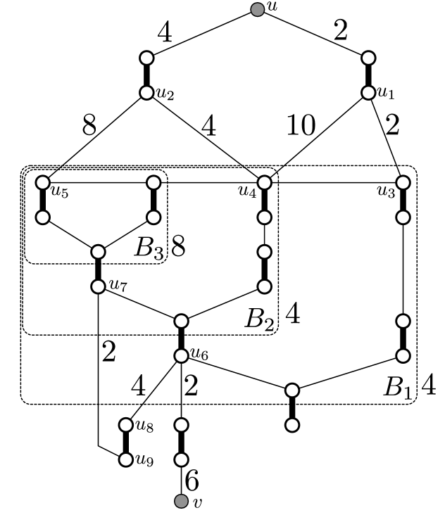
Figure 9: Edges are labeled with their initial slack; blossoms are labeled with their $z$-values.

At time zero $u$ is outer and all other vertices are not in the search structure.

At time 2 $u_{1}$ becomes outer and the edges $(u_{1},u_{3})$ and $(u_{1},u_{4})$ are scanned. Both edges connect to blossom $B_{1}$ and $(u_{1},u_{3})$ has less slack, but, as we shall see, $(u_{1},u_{4})$ cannot be discarded at this point.

At time 4 $B_{1}$ becomes an inner blossom and $u_{2}$ becomes outer, causing $(u_{2},u_{4})$ and $(u_{2},u_{5})$ to be scanned. Note that since $u_{4}$ is inner (as part of $B_{1}$), further dual adjustments will not change the slack on $(u_{2},u_{4})$ (slack 4) or $(u_{1},u_{4})$ (now slack 8). Nonetheless, in the future $u_{4}$ may not be in the search structure, so we note that the edge with least slack incident to it is $(u_{2},u_{4})$ and discard $(u_{1},u_{4})$.

At time 6 $B_{1}$ dissolves: the path from $u_{3}$ to $B_{1}$’s base enters the search structure and everything else ($B_{2}$ and $u_{6}$) are split off. At this point further dual adjustments do change the slack on edges incident to $B_{2}$.

At time 10 $(u_{2},u_{4})$ becomes tight, $B_{2}$ becomes inner and $u_{6}$ becomes outer. At time 12 $B_{2}$ dissolves. At this point $u_{6}$ has experienced 2 dual adjustments as an inner vertex (as part of $B_{1}$) and 2 dual adjustments as an outer vertex, while $u_{7}$ has experienced 4 dual adjustments as an inner vertex (as part of $B_{1}$ and $B_{2}$). Thus, the slacks on $(u_{6},u_{8})$ and $(u_{7},u_{9})$ are 4 and 6 respectively.

At time 16 $(u_{2},u_{5})$ and $(u_{6},u_{8})$ become tight, making $B_{3}$ inner and $u_{7}$ and $u_{9}$ outer. The edge $(u_{7},u_{9})$ still has slack 6. At time 19 $(u_{7},u_{9})$ becomes tight, forming a new blossom $B_{4}$ based at $u_{2}$. At time 20 the final edge on the augmenting path from $u$ to $v$ becomes tight.

Observe that a vertex can enter into and exit from the search structure an unbounded number of times. Merely calculating a vertex’s current $y$-value requires that we consider the entire history of the vertex’s involvement in the search structure. For example, $u_{5}$ participated as an inner vertex in dual adjustments during the intervals $[4,6),[10,12),$ and $[16,19)$ and as an outer vertex during $[19,20)$.

5.1 An Overview of the Data Structures

In order to implement Edmonds’ algorithm efficiently we need to address three data structuring problems:

1. a union-find type data structure for maintaining the (growing) outer blossoms. This data structure is used to achieve two goals. First, whenever an outer-outer edge $e=(u,u^{\prime})$ is scanned (like $(u_{7},u_{9})$ in the example), we need to tell whether $u,u^{\prime}$ are in the same outer blossom, in which case $e$ is ignored, or whether they are in different blossoms, in which case we must schedule a blossom formation event after $\operatorname{slack}(e)/2$ further dual adjustments. Second, when forming an outer blossom, we need to traverse its odd cycle in time proportional to its length in the contracted graph. E.g., when $(u_{7},u_{9})$ triggers the formation of $B_{4}$, we walk up from $u_{7}$ and $u_{9}$ to the base $u_{2}$ enumerating the vertices/root blossoms encountered. The walk must “hop” from $u_{7}$ to $u_{5}$ (representing $B_{3}$), without spending time proportional to $|B_{3}|$.

2. a split-findmin data structure for maintaining the (dissolving) inner blossoms. The data structure must be able to dissolve an inner blossom into the components along its odd cycle. It must be able to determine the edge with minimum slack connecting an inner blossom to an outer vertex, and to do the same for individual vertices in the blossom. For example, when $(u_{2},u_{4})$ is scanned we must check whether its slack is better than the other edges incident to $u_{4}$, namely $(u_{1},u_{4})$.

3. a priority queue for scheduling three types of events: blossom dissolutions, blossom formations, and grow steps, which add a new (tight) edge and vertex to the search structure.

Before we get into the implementation details let us first make some remarks on the existing options for (1)–(3).

A standard union-find algorithm will solve (1) in $O(m\alpha(m,n)+n)$ time. Gabow and Tarjan [18] observed that a special case of union-find can be solved in $O(m+n)$ time if the data structure gets commitments on future union operations. Let $\{\{1\},\{2\},\ldots,\{n\}\}$ be the initial set partition and $T=\emptyset$ be an edge set on the vertex set $\{1,\ldots,n\}$. We must maintain the invariant that $T$ is a single connected tree at all times. The data structure handles intermixed sequences of three operations.

• $\mathsf{addedge}(u,v)$ : $T\leftarrow T\cup\{(u,v)\}$.
  It is required that $T$ is connected. If $v$ was previously not in $T$, record $u$ as the parent of $v$.

• $\mathsf{unite}(u,v)$ : Replace the sets containing $u$ and $v$ with their union.
  This is only permitted if $(u,v)\in T$.

• $\mathsf{find}(u)$ : Find the representative of $u$’s set.

It is not too difficult to cast Edmonds’ search in this framework. We explain exactly how in Section 5.2.

Gabow introduced the split-findmin structure in [13] to manage blossom dissolutions in Edmonds’ algorithm, but did not fully specify how it should be applied. The data structure maintains a set $\mathcal{L}$ of lists of elements, each associated with a key. It supports the following operations.

• $\mathsf{init}(u_{1},\ldots,u_{n})$ : Set $\mathcal{L}\leftarrow\{(u_{1},\ldots,u_{n})\}$ and $\operatorname{key}(u_{i})\leftarrow\infty$ for all $i$.

• $\mathsf{list}(u)$ : Return a pointer to the list in $\mathcal{L}$ containing $u$.

• $\mathsf{split}(u)$ : Suppose $\mathsf{list}(u)=(u^{\prime},\ldots,u,u^{\prime\prime},\ldots,u^{\prime\prime\prime})$. Update $\mathcal{L}$ as follows:

  $$\mathcal{L}\leftarrow\mathcal{L}\,\backslash\,\{\mathsf{list}(u)\}\cup\{(u^{\prime},\ldots,u),\;(u^{\prime\prime},\ldots,u^{\prime\prime\prime})\}.$$

• $\mathsf{decreasekey}(u,x)$ : Set $\operatorname{key}(u)\leftarrow\min\{\operatorname{key}(u),x\}$.

• $\mathsf{findmin}(L\in\mathcal{L})$ : Return $\min_{u\in L}\operatorname{key}(u)$.

The idea is that $\mathsf{init}$ should be called with a permutation of the vertex set such that each initial blossom (maximal or not) is contiguous in the list. Splits are performed whenever necessary to maintain the invariant that non-outer root blossoms are identified with lists in $\mathcal{L}$. The value $\operatorname{key}(u)$ is used to encode the minimum slack of any edge $(v,u)$ ($v$ outer) incident to $u$. We associate other useful information with elements and lists; for example, $u$ stores a pointer to the edge $(v,u)$ corresponding to $\operatorname{key}(u)$.

Pettie [32] improved the running time of Gabow’s split-findmin structure from $O(m\alpha(m,n)+n)$ to $O(m\log\alpha(m,n)+n)$, $m$ being the number of $\mathsf{decreasekey}$ operations. Thorup [33] showed that with integer keys, split-findmin could be implemented in optimal $O(m+n)$ time using atomic heaps [11].

For (3) we can use a standard priority queue supporting insert and deletemin. Note however, that although there are ultimately only $O(n)$ events, we may execute $\Theta(n+m)$ priority operations. The algorithm may schedule $\Omega(m)$ blossom formation events but, when each is processed, discover that the endpoints of the edge in question have already been contracted into the same outer blossom. (A decreasekey operation, if it is available, is useful for rescheduling grow events but cannot directly help with blossom formation events.) Gabow’s specialized priority queue [15] schedules all blossom formation events in $O(m+n\log n)$ time. Unfortunately, the $\Omega(n\log n)$ term in Gabow’s data structure cannot be reduced if the edge weights happen to be small integers. Let $t_{\max}$ be the maximum number of dual adjustments performed by a search. In the BucketSearch implementation we shall allocate an array of $t_{\max}$ buckets to implement the priority queue, bucket $i$ being a linked list of events scheduled for time $i$. With this implementation all priority queue operations take $O(1)$ time, plus $O(t_{\max})$ for scanning empty buckets. When $t_{\max}$ is unknown/unbounded we use a general integer priority queue [23, 24, 35] and call the implementation PQSearch.

In the remainder of this section we explain how to implement Edmonds’ search procedure using the data structures mentioned above. This is presumably close to the implementation that Gabow [13] had in mind, but it is quite different from the other $\tilde{O}(m)$ implementations of [21, 17, 15]. Theorem 5.1 summarizes the properties of this implementation.

Theorem 5.1.

The time to perform Edmonds’ search procedure on an integer-weighted graph, using specialized union-find [18], split-findmin [33], and priority queue [23, 24, 35] data structures, is $O(m+t)$ (where $t$ is the number of dual adjustments, using a trivial priority queue) or $O(m\log\log n)$ (using [23, 35]) or $O(m\sqrt{\log\log n})$ with high probability (using [24, 35]). On real-weighted graphs the time is $O(m+n\log n)$ using [15], or $O(m\log n)$ using any $O(\log n)$-time priority queue.

5.2 Implementation Details

We explicitly maintain the following quantities, for each $v$ and each blossom $B$. A vertex $B$ not in any blossom is considered a root blossom, trivially.

$$t_{\operatorname{now}} =\mbox{The current {\em time}. (The number of dual adjustments performed so far.)}$$

$$y_{0}(v) =\mbox{The initial value of $y(v)$.}$$

$$z_{0}(B) =\mbox{The initial value of $z(B)$ ($B$ not necessarily a root blossom).}$$

$$t_{\operatorname{root}}(B) =\mbox{The time $B$ became a root blossom.}$$

$$t_{\operatorname{in}}(B) =\mbox{The time $B$ became an inner root blossom.}$$

$$t_{\operatorname{out}}(B) =\mbox{The time $B$ became (part of) an outer root blossom.}$$

$$\Delta(B) =\mbox{The number of dual adjustments experienced by vertices in $B$ as inner vertices,}$$

in the interval $$[0,\max\{t_{\operatorname{root}}(B),t_{\operatorname{out}}(B)\}]$$.

It is straightforward to keep these values up to date. To give a sense of what is involved, we illustrate how they change in two cases: when an inner blossom dissolves and when an outer blossom is formed. Whenever an inner blossom $$B^{\prime} B$$ is dissolved we visit each subblossom on its odd-cycle and set

$$t_{\operatorname{root}}(B) \leftarrow t_{\operatorname{now}}$$

$$\Delta(B) \leftarrow\Delta(B^{\prime})+(t_{\operatorname{now}}-t_{\operatorname{in}}(B^{\prime}))$$

and if $$B t_{\operatorname{in}}(B)\leftarrow t_{\operatorname{now}} t_{\operatorname{out}}(B)\leftarrow t_{\operatorname{now}} B^{\prime} B B$$ is immediately inserted into the search structure as an inner or outer blossom we set or accordingly. When an outer blossom is created we visit each subblossom on its odd-cycle. For each formerly inner , we update its values as follows

$$t_{\operatorname{out}}(B) \leftarrow t_{\operatorname{now}}$$

$$\Delta(B) \leftarrow\Delta(B)+(t_{\operatorname{now}}-t_{\operatorname{in}}(B))$$

From these quantities we can calculate the current $$y z \mathsf{split} \mathsf{list}(v)=B v v v$$- and -values as follows. Remember that s are performed so that was the last root blossom containing just before became outer, or the current root blossom containing if it is non-outer.

$$y(v) =\makebox[0.0pt][l]{$y_{0}(v)$}\;\;\;\;\;\;\;\;\;+\left\{\begin{array}[]{l@{\hcm[.3]}l}\makebox[0.0pt][l]{$\Delta(B)+t_{\operatorname{now}}-t_{\operatorname{in}}(B)$}\hfil\hskip 8.5359pt&\mbox{ if $B=\mathsf{list}(v)$ is an inner root blossom}\\ \makebox[0.0pt][l]{$\Delta(B)-(t_{\operatorname{now}}-t_{\operatorname{out}}(B))$}\hfil\hskip 8.5359pt&\mbox{ if $B=\mathsf{list}(v)$ is in an outer blossom}\\ \makebox[0.0pt][l]{$\Delta(B)$}\hfil\hskip 8.5359pt&\mbox{ otherwise}\end{array}\right.$$

$$z(B) =\makebox[0.0pt][l]{$z_{0}(B)$}\;\;\;\;\;\;\;\;\;+\left\{\begin{array}[]{l@{\hcm[.3]}l}\makebox[0.0pt][l]{$0$}\hfil\hskip 8.5359pt&\mbox{ if $t_{\operatorname{root}}(B)$ is undefined}\\ \makebox[0.0pt][l]{$-2\Delta(B)-2(t_{\operatorname{now}}-t_{\operatorname{in}}(B))$}\hfil\hskip 8.5359pt&\mbox{ if $B$ is an inner root blossom}\\ \makebox[0.0pt][l]{$-2\Delta(B)+2(t_{\operatorname{now}}-t_{\operatorname{out}}(B))$}\hfil\hskip 8.5359pt&\mbox{ if $B$ is in an outer blossom}\end{array}\right.$$

Note that if $$B z_{0}(B)=\Delta(B)=0 (u,v) \operatorname{slack}(u,v)=y(u)+y(v)-w(u,v) \operatorname{slack}^{\star}(u,v)$$ was not a weighted blossom at time zero, . The slack of an edge not in any blossom is calculated as . However, when using Criteria 2 or 3 of eligibility we really want to measure the distance from the edge being eligible. Define as follows.

$$\operatorname{slack}^{\star}(e) =\left\{\begin{array}[]{ll}\operatorname{slack}(e)&\mbox{ Criterion~{}\ref{crit1}}\\ \operatorname{slack}(e)+2&\mbox{ Criterion~{}\ref{crit2} and $e\not\in M$}\\ -\operatorname{slack}(e)&\mbox{ Criterion~{}\ref{crit2} and $e\in M$}\\ \operatorname{slack}(e)&\mbox{ Criterion~{}\ref{crit3} and $\operatorname{slack}(e)\geq 0$}\\ \operatorname{slack}(e)+2&\mbox{ Criterion~{}\ref{crit3} and $\operatorname{slack}(e)\in\{-1,-2\}$}\end{array}\right.$$

Dual adjustments can change the slack of many edges, but we can only afford to update the split-findmin structure when edges are scanned. We maintain the invariant that if $u$ is not in an outer blossom, $\operatorname{key}(u)$ is equal to $\min_{\operatorname{outer}\;v}\operatorname{slack}^{\star}(v,u)$, up to some offset that is common to all vertices in $\mathsf{list}(u)$. Consider an edge $(v,u)$ with $v$ outer and $u$ non-outer. When $u$ is not in the search structure each dual adjustment reduces the slack on $(v,u)$ whereas when $u$ is inner each dual adjustment has no effect. We maintain the following invariant for each non-outer element $u$ in the split-findmin structure.

$$\min_{\operatorname{outer}\;v}\operatorname{slack}^{\star}(v,u) =\left\{\begin{array}[]{l@{\hcm[1]}l}\operatorname{key}(u)-(t_{\operatorname{in}}(B)-\Delta(B))\hfil\hskip 28.45274pt&\mbox{ if $B=\mathsf{list}(u)$ is inner}\\ \operatorname{key}(u)-(t_{\operatorname{now}}-\Delta(B))\hfil\hskip 28.45274pt&\mbox{ if $B=\mathsf{list}(u)$ is neither inner nor outer}\end{array}\right.$$

Let $F$ be the set of free vertices that we are conducting the search from. In accordance with our earlier assumptions we assume that $\{y_{0}(v)\;|\;v\in F\}$ have the same parity and that all edge weights are even. We will grow a forest $T$ of $|F|$ trees, each rooted at an $F$-vertex, such that the outer blossoms form connected subtrees of $T$, thereby allowing us to apply the union-find algorithm [18] to each tree. Let $\operatorname{rt}(u)$ be the free vertex at the root of $u$’s tree. We initialize the split-findmin structure to reflect the structure of initial blossoms at time $t_{\operatorname{now}}=0$ and call $\mathsf{grow}(v,\perp)$ for each $v\in F$. In general, we iteratively process any events scheduled for $t_{\operatorname{now}}$, incrementing $t_{\operatorname{now}}$ when there are no such events. Eventually an augmenting path will be discovered (during the course of processing a grow or blossom formation event) or the priority queue becomes empty, in which case we conclude that there are no augmenting paths from any vertices in $F$.

The $\mathsf{grow}(v,e)$ procedure.

The first argument ($v$) is a new vertex to be added to the search structure. The second argument $e=(u,v)$ is an edge with $\operatorname{slack}^{\star}(e)=0$ connecting $v$ to an existing $u$ in the search structure, or $\perp$ if $v$ is free. If $e\neq\perp$ we begin by calling $\mathsf{addedge}(e)$.

We first consider the case when $e\in M$ or $e=\perp$, so $v$ is designated outer. If $v$ is not contained in any blossom we call $\mathsf{schedule}(v)$ to schedule grow and blossom formation events for all unmatched edges incident to $v$. If $B=\mathsf{list}(v)$ is a non-trivial (outer) blossom we call $\mathsf{addedge}(v^{\prime},v)$ and $\mathsf{unite}(v^{\prime},v)$, for each $v^{\prime}\in B\backslash\{v\}$, then call $\mathsf{schedule}(v^{\prime})$ for each $v^{\prime}\in B$. (Recall that in order to apply [18], the members of every outer blossom must form a contiguous subset of $T$.)

Suppose $e=(u,v)\not\in M$ and that $v$ is not contained in any blossom. If $v$ is free then we have found an augmenting path and are done. Otherwise we call $\mathsf{schedule}(v)$ to schedule the grow step for $v$’s matched edge. If $B=\mathsf{list}(v)$ is a non-trivial (inner) blossom, find the base $b$ of $B$ and the even-length path $P$ from $v$ to $b$ in $E_{B}$, in $O(|P|)$ time. For each edge $e\in P$ call $\mathsf{addedge}(e)$ in order to include $P$ in $T$. If $b$ is free then we have found an augmenting path; if not then we call $\mathsf{schedule}(b)$ to schedule $B$’s blossom dissolution event and the grow event for $b$’s matched edge.

The $\mathsf{schedule}(u)$ procedure.

The purpose of this procedure is to schedule future events associated with $u$ or edges incident to $u$. First consider the case when $u$ is inner. If $B=\mathsf{list}(u)$ is a non-trivial blossom we schedule a $\mathsf{dissolve}(B)$ event at time $t_{\operatorname{now}}+z_{0}(B)/2$. Let $e=(u,v)\in M$ be the matched edge incident to $u$. If $v$ is neither inner nor outer then schedule a $\mathsf{grow}(v,e)$ event at time $t_{\operatorname{now}}+\operatorname{slack}^{\star}(e)$. If $v$ is currently inner we cancel the existing event for $\mathsf{grow}(u,e)$ and schedule a $\mathsf{blossom}(e)$ event at time $t_{\operatorname{now}}+\operatorname{slack}^{\star}(e)/2$.

When $u$ is outer we perform the following steps for each unmatched edge $e=(u,v)\in E(G)$. If $\mathsf{find}(u)=\mathsf{find}(v)$ then $(u,v)$ can be discarded. If $v$ is also outer and $\mathsf{find}(u)\neq\mathsf{find}(v)$ then schedule a $\mathsf{blossom}(e)$ event at time $t_{\operatorname{now}}+\operatorname{slack}^{\star}(e)/2$. If $v$ is inner let $(u^{\prime},v)$ be the existing edge with $u^{\prime}$ outer minimizing $\operatorname{slack}^{\star}(u^{\prime},v)$. If $\operatorname{slack}^{\star}(e)<\operatorname{slack}^{\star}(u^{\prime},v)$ then we perform a $\mathsf{decreasekey}(v,x)$ operation with the new key $x$ corresponding to $\operatorname{slack}^{\star}(e)$. If $B=\mathsf{list}(v)$ is neither inner nor outer and updating $\operatorname{key}(v)$ causes $\mathsf{findmin}(B)$ to change, we cancel the existing grow event associated with $B$ and schedule $\mathsf{grow}(v,e)$ for time $t_{\operatorname{now}}+\operatorname{slack}^{\star}(e)$.

The $\mathsf{dissolve}(B)$ procedure.

Let $P=T\cap E_{B}$ be the even-length alternating path from some $v\in B$ to the base $b$ of $B$. For each subblossom $B^{\prime}$ on $B$’s odd cycle we call $\mathsf{split}(u^{\prime})$ on the last vertex $u^{\prime}\in B$, thereby splitting $B$ into its constituents. The subblossoms $B^{\prime}$ are of three kinds: they either (i) intersect $P$ as inner vertices/blossoms, (ii) intersect $P$ as outer vertices/blossoms, or (iii) do not intersect $P$. If $B^{\prime}$ is of type (i) then subsequent dual adjustments will reduce $z(B^{\prime})$. We schedule a $\mathsf{dissolve}(B^{\prime})$ event for time $t_{\operatorname{now}}+z_{0}(B^{\prime})/2$. If $B^{\prime}$ is type (ii) let $b^{\prime}$ be its base. Every vertex $v^{\prime}\in B^{\prime}$ is now outer. For each $v^{\prime}\in B^{\prime}\backslash\{b^{\prime}\}$ we call $\mathsf{addedge}(v^{\prime},b^{\prime}),\mathsf{unite}(v^{\prime},b^{\prime})$ and for each $v^{\prime}\in B^{\prime}$ we call $\mathsf{schedule}(v^{\prime})$ to schedule events for unmatched edges incident to $v^{\prime}$. When $B^{\prime}$ is type (iii) we call $\mathsf{findmin}(B^{\prime})$ to determine the unmatched edge $e=(u,v)$ ($u$ outer, $v\in B^{\prime}$) minimizing $\operatorname{slack}^{\star}(u,v)$. We schedule a $\mathsf{grow}(v,e)$ event at time $t_{\operatorname{now}}+\operatorname{slack}^{\star}(u,v)$.

The $\mathsf{blossom}(u,v)$ procedure.

When a $\mathsf{blossom}(u,v)$ event occurs either $\operatorname{slack}^{\star}(u,v)=0$ or $u$ and $v$ have already been contracted into a common outer blossom. If $\mathsf{find}(u)=\mathsf{find}(v)$ we are done. If $\operatorname{rt}(u)\neq\operatorname{rt}(v)$ then we have discovered an eligible augmenting path from $\operatorname{rt}(u)$ to $\operatorname{rt}(v)$ via $(u,v)$. If $\operatorname{rt}(u)=\operatorname{rt}(v)$ then a new blossom $B$ must be formed. The base of $b$ will be the least common ancestor of $u$ and $v$ in $T$. We walk from $u$ up to $b$ and from $v$ up to $b$, making sure that all members of $B$ are in the same set defined by $\mathsf{unite}$ operations. Here we must be more specific about which vertex in a blossom is the “representative” returned by $\mathsf{find}(\cdot)$. The representative of a blossom is its most ancestral node in $T$. For outer blossoms this is always the base; for inner blossoms this is the vertex $v$ in the call to $\mathsf{grow}(v,(u,v))$ that caused $v$’s blossom to become inner.

Let $u^{\prime}$ be the current vertex under consideration on the path from $u$ to $b$. If $u^{\prime}$ is outer, in a non-trivial blossom, but not the base of the blossom, set $u^{\prime}\leftarrow\mathsf{find}(u^{\prime})$ to be the base of the blossom and continue. Suppose $u^{\prime}$ is the base of an outer blossom and $v^{\prime}$ is its (inner) parent. Call $\mathsf{unite}(u^{\prime},v^{\prime})$; set $u^{\prime}\leftarrow v^{\prime}$ and continue. If $u^{\prime}$ is inner, not in any blossom, and $v^{\prime}$ is its parent, call $\mathsf{unite}(u^{\prime},v^{\prime})$; set $u^{\prime}\leftarrow v^{\prime}$ and continue. Suppose $u^{\prime}$ is in a non-trivial inner blossom $B^{\prime}=\mathsf{list}(u^{\prime})$. Let $P^{\prime}=E_{B^{\prime}}\cap T$ be the (possibly empty) path from $u^{\prime}$ to the representative $v^{\prime}$ of $B^{\prime}$ and let $u^{\prime\prime}$ be the parent of $v^{\prime}$. Call $\mathsf{unite}(e)$ for each $e\in P^{\prime}$ then, for each $v^{\prime\prime}\in B^{\prime}\backslash V(P^{\prime})$, call $\mathsf{addedge}(v^{\prime\prime},v^{\prime})$ and $\mathsf{unite}(v^{\prime\prime},v^{\prime})$. Call $\mathsf{unite}(v^{\prime},u^{\prime\prime})$; set $u^{\prime}\leftarrow u^{\prime\prime}$ and continue. The same procedure is repeated on the path from $v$ up to $b$. Note that the time required to construct $B$ is linear in the number of $B$-vertices that make the transition from inner to outer. Thus, the total time for forming all outer blossoms is $O(n)$.

For each $v^{\prime}\in B$ that was not already outer before the formation of $B$, call $\mathsf{schedule}(v^{\prime})$ to schedule events for unmatched edges incident to $v^{\prime}$.

5.3 Postprocessing

Once a single augmenting path is found we explicitly record all $y$- and $z$-values, in $O(n)$ time. At this moment the (relaxed) complementary slackness invariants (Property 1 or 2) are satisfied, except possibly the Active Blossom invariant. Any blossoms that were formed at the same time that the first augmenting path was discovered will have zero $z$-values. Also, a non-root blossom with zero $z$-value may become a root blossom just as the first augmenting path is found. Thus, we must dissolve root blossoms with zero $z$-values as long as they exist.

6 Conclusion

We have presented a new scaling algorithm for mwpm on general graphs that runs in $O(m\sqrt{n}\log(nN))$ time. This algorithm improves slightly on the running time of the Gabow-Tarjan algorithm [20]. However, its analysis is simpler than [20] and is generally more accessible. Historically there were two barriers to computing weighted matching in less than $O(m\sqrt{n}\log(nN))$ time. The first barrier was that the best cardinality matching algorithms took $O(m\sqrt{n})$ time [36, 37, 20, 16], and cardinality matching seems easier than a single scale of weighted matching. The second barrier was that even on bipartite graphs, where blossoms are not an issue, the best matching algorithms took $O(m\sqrt{n}\log(nN))$ time [19, 30, 22, 6]. Recent work by Cohen, Mądry, Sankowski, and Vladu [2] has broken the second barrier on sufficiently sparse graphs. They showed that several problems, including weighted bipartite matching, can be computed in $\tilde{O}(m^{10/7}\log N)$ time.

We highlight several problems left open by this work.

• The Liquidationist mwpm algorithm is relatively simple and streamlined, and among the scaling algorithms for mwpm so-far proposed [13, 20], the one with the clearest potential for practical impact. However, on sparse graphs it is theoretically an $O(\sqrt{\log\log n})$ factor slower than the Hybrid algorithm. Can the efficiency of Hybrid be matched by an algorithm that is as simple as Liquidationist?

• There is now some evidence that the maximum weight (not necessarily perfect) matching problem [6, 31, 25, 26] may be slightly easier than mwpm. Is it possible to compute a maximum weight matching of a general graph in $O(m\sqrt{n}\log N)$ time, matching the bound of Duan and Su [6] for bipartite graphs?

• The implementation of Edmonds’ algorithm described in Section 5 uses an (integer) priority queue supporting insert and delete-min, but does not take advantage of fast decrease-keys. Given an integer priority queue supporting $O(1)$ time decrease-key and $O(q)$ time insert and delete-min, is it possible to implement Edmonds’ search in $O(m+nq)$ time, matching the bound for a Hungarian search [10, 34] on a bipartite graph?

Acknowledgement.

We would like to thank the two anonymous reviewers, whose careful reading lead to numerous improvements to the presentation.

References

- [1] G. Birkhoff. Tres observaciones sobre el elgebra lineal. Universidad Nacional de Tucuman, Revista A, 5(1–2):147–151, 1946.
- [2] M. B. Cohen, A. Madry, P. Sankowski, and A. Vladu. Negative-weight shortest paths and unit capacity minimum cost flow in time. In Proceedings 28th Annual ACM-SIAM Symposium on Discrete Algorithms (SODA), pages 752–771, 2017.
- [3] W. H. Cunningham and A. B. Marsh, III. A primal algorithm for optimum matching. Mathematical Programming Study, 8:50–72, 1978.
- [4] M. Cygan, H. N. Gabow, and P. Sankowski. Algorithmic applications of Baur-Strassen’s theorem: Shortest cycles, diameter, and matchings. J. ACM, 62(4):28, 2015.
- [5] R. Duan and S. Pettie. Linear-time approximation for maximum weight matching. J. ACM, 61(1):1, 2014.
- [6] R. Duan and H.-H. Su. A scaling algorithm for maximum weight matching in bipartite graphs. In Proceedings 23rd ACM-SIAM Symposium on Discrete Algorithms (SODA), pages 1413–1424, 2012.
- [7] J. Edmonds. Maximum matching and a polyhedron with -vertices. J. Res. Nat. Bur. Standards Sect. B, 69B:125–130, 1965.
- [8] J. Edmonds. Paths, trees, and flowers. Canadian Journal of Mathematics, 17:449–467, 1965.
- [9] J. Edmonds and R. M. Karp. Theoretical improvements in algorithmic efficiency for network flow problems. J. ACM, 19(2):248–264, 1972.
- [10] M. L. Fredman and R. E. Tarjan. Fibonacci heaps and their uses in improved network optimization algorithms. J. ACM, 34(3):596–615, 1987.
- [11] M. L. Fredman and D. E. Willard. Trans-dichotomous algorithms for minimum spanning trees and shortest paths. J. Comput. Syst. Sci., 48(3):533–551, 1994.
- [12] H. N. Gabow. An efficient implementation of Edmonds’ algorithm for maximum matching on graphs. J. ACM, 23:221–234, April 1976.
- [13] H. N. Gabow. A scaling algorithm for weighted matching on general graphs. In Proc. 26th Annual Symposium on Foundations of Computer Science (FOCS’85), pages 90–100, 1985.
- [14] H. N. Gabow. Data structures for weighted matching and nearest common ancestors with linking. In Proceedings First Annual ACM-SIAM Symposium on Discrete Algorithms (SODA), pages 434–443, 1990.
- [15] H. N. Gabow. Data structures for weighted matching and extensions to -matching and -factors. CoRR, abs/1611.07541, 2016.
- [16] H. N. Gabow. The weighted matching approach to maximum cardinality matching. Fundam. Inform., 154(1–4):109–130, 2017.
- [17] H. N. Gabow, Z. Galil, and T. H. Spencer. Efficient implementation of graph algorithms using contraction. J. ACM, 36(3):540–572, 1989.
- [18] H. N. Gabow and R. E. Tarjan. A linear-time algorithm for a special case of disjoint set union. J. Comput. Syst. Sci., 30(2):209–221, 1985.
- [19] H. N. Gabow and R. E. Tarjan. Faster scaling algorithms for network problems. SIAM J. Comput., 18(5):1013–1036, 1989.
- [20] H. N. Gabow and R. E. Tarjan. Faster scaling algorithms for general graph-matching problems. J. ACM, 38(4):815–853, 1991.
- [21] Z. Galil, S. Micali, and H. N. Gabow. An algorithm for finding a maximal weighted matching in general graphs. SIAM J. Comput., 15(1):120–130, 1986.
- [22] A. V. Goldberg and R. Kennedy. Global price updates help. SIAM J. Discr. Math., 10(4):551–572, 1997.
- [23] Y. Han. Deterministic sorting in time and linear space. In Proc. 34th ACM Symp. on Theory of Comput. (STOC), pages 602–608. ACM Press, 2002.
- [24] Y. Han and M. Thorup. Integer sorting in expected time and linear space. In Proc. 43rd Symp. on Foundations of Computer Science (FOCS), pages 135–144, 2002.
- [25] C.-C. Huang and T. Kavitha. Efficient algorithms for maximum weight matchings in general graphs with small edge weights. In Proceedings of the Twenty-Third Annual ACM-SIAM Symposium on Discrete Algorithms (SODA), pages 1400–1412, 2012.
- [26] M.-Y. Kao, T. W. Lam, W.-K. Sung, and H.-F. Ting. A decomposition theorem for maximum weight bipartite matchings. SIAM J. Comput., 31(1):18–26, 2001.
- [27] A. V. Karzanov. Efficient implementations of Edmonds’ algorithms for finding matchings with maximum cardinality and maximum weight. In A. A. Fridman, editor, Studies in Discrete Optimization, pages 306–327. Nauka, Moscow, 1976.
- [28] E. Lawler. Combinatorial Optimization: Networks and Matroids. Holt, Rinehart & Winston, New York, 1976.
- [29] S. Micali and V. Vazirani. An algorithm for finding maximum matching in general graphs. In Proc. 21st IEEE Symposium on Foundations of Computer Science (FOCS), pages 17–27, 1980.
- [30] J. B. Orlin and R. K. Ahuja. New scaling algorithms for the assignment and minimum mean cycle problems. Math. Program., 54:41–56, 1992.
- [31] S. Pettie. A simple reduction from maximum weight matching to maximum cardinality matching. Inf. Process. Lett., 112(23):893–898, 2012.
- [32] S. Pettie. Sensitivity analysis of minimum spanning trees in sub-inverse-Ackermann time. J. Graph Algorithms and Applications, 19(1):375–391, 2015.
- [33] M. Thorup. Undirected single-source shortest paths with positive integer weights in linear time. J. ACM, 46(3):362–394, 1999.
- [34] M. Thorup. Integer priority queues with decrease key in constant time and the single source shortest paths problem. In Proc. 35th ACM Symp. on Theory of Computing (STOC), pages 149–158, 2003.
- [35] M. Thorup. Equivalence between priority queues and sorting. J. ACM, 54(6), 2007.
- [36] V. V. Vazirani. An improved definition of blossoms and a simpler proof of the MV matching algorithm. CoRR, abs/1210.4594, 2012.
- [37] V. V. Vazirani. A proof of the MV matching algorithm. In submission, 2014.
- [38] J. von Neumann. A certain zero-sum two-person game equivalent to the optimal assignment problem. In H. W. Kuhn and A. W. Tucker, editors, Contributions to the Theory of Games, volume II, pages 5–12. Princeton University Press, 1953.