The Spherical Ratio of Two Points
and Its Integral Properties
Abstract
At the end of 19-th century, 1874, Hermann Schwartz found that for every point inside a planar disk, a two-dimensional Poisson Kernel can be written as a ratio of two segments, which he called as the geometric interpretation of that Kernel [1]. About 90 years later, Lars Ahlfors, in his textbook, called this ratio as interesting [2]. We shall see here that every two different points, in a multidimensional space also define a similar ratio of two segments. The main goal of this paper is to study some integral properties of the ratio as well as introduce and proof One Radius Theorem for Spherical Ratio of two points. In particular, we introduce a new integration technique involving the ratio of two segments and a non-trivial integral equivalence leading to an integral relationship between Newtonian Potential and Poisson Kernel in any multi-dimensional space.
1 Introduction
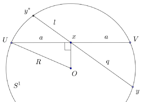
In this paper we introduce a new mathematical value , called the spherical ratio of two points. Such ratio is a generalization of the ratio of two segments originally introduced by Hermann Schwartz at the end of 19-th century, ([1], pp. 359-361) or ([2], pp. 168-169). While studying complex analysis, he found that for a point inside a planar disk, the Poisson Kernel can be written as a ratio of two segments. For the notations in the formula below, look at Figure 1.
| (1) |
We shall see that a similar ratio can be defined for every two different points in a multidimensional space and can serve as a useful tool for integration of some functions over sphere. The technique of integration together with the results obtained here can be applied for spectral analysis in a hyperbolic space. This happens because the ratio of two segments represents an eigenfunction of the hyperbolic Laplacian, while the averaging of over sphere represents a radial eigenfunction of the hyperbolic Laplacian. Therefore, all statements obtained in this paper can be restated in terms of radial eigenfunctions and used to obtain some results related, for example, to Dirichlet Eigenvalue Problem in a disc of constant negative curvature.
The main goal of this article is to describe the constraints for complex numbers and for a fixed point under which the following equivalence holds.
| (2) |
where is the spherical ratio of two points that is defined below.
2 Definitions and Basic Results
Definition 2.1 (Spherical Ratio of Two Points).
Let and assume that . Let denotes the -dimensional sphere of radius centered at the origin . Then, let us introduce and as follows. If the line defined by and is tangent to , then we set . Otherwise, be the point of such that and are collinear. Note that in case . Similarly, if the line through is tangent to , then we set . Otherwise, be the point of such that and are collinear. Note again that in the case . Then, we can observe that and denote
We call the ratio of these two segments and , as the spherical ratio of two points and , i.e.,
| (3) |
where the last expression is exactly the 2-D Poisson Kernel for a planar disk.
Corollary 2.2.
Theorem 2.3 (One Radius Theorem for ).
Let , , be a -dimensional sphere of radius centered at the origin , such that and is defined in (3). Until further notice we assume that and a point are fixed. Then, the following Statements hold.
- (A)
-
If and , then
(4) - (B)
-
If are real, then
(5) - (C)
-
For every there are infinitely many numbers such that
(6) - (D)
-
Suppose that for the fixed point
(7) Then
(8)
Remark 2.4.
Remark 2.5.
Observe that Statement (B) is a special case of Statement (D). Indeed, if are real, then (7) holds for every .
Corollary 2.6.
| (9) |
Moreover, for every natural number
| (10) |
and for every
| (11) |
which is the Taylor decomposition of at .
Corollary 2.7.
If and , then
| (12) |
Remark 2.8.
It is clear that formula (12) can be obtained from Statement (A) if we rewrite formula (4) in terms of distance between and . In particular, for and for every , formula (12) yields
| (13) |
Note that for the integrand on the left is the Newtonian potential in and the integrand on the right is exactly the Poisson kernel in .
Corollary 2.9.
If , then for every and ,
| (14) |
Corollary 2.10.
If , then
| (15) |
In particular, if ,
| (16) |
3 Proof of the basic results
Proof of Theorem 2.3..
We are going to prove successively all of the Statements (A), (B), (C) and (D) from the Theorem.
Proof of Statement (A), p. (A)..
Case 1 (). For notation refer to Figure 2. Let be an arbitrary point of . Here, is defined as an intersection of the sphere and line . Angle is defined as and is defined as . The circle appears on the cross-sectional plane defined by the points , and . Let and and let the segments be perpendicular to .
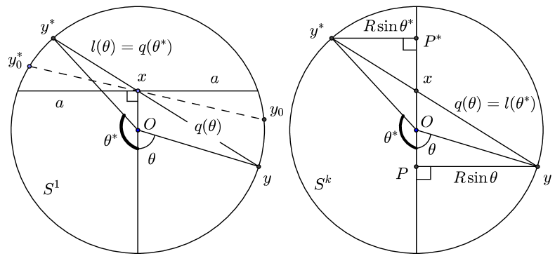
One can easily check that
| (17) |
since and, by Pythagorean theorem, .
In the next step we are going to use the change of variables from to , introduced also by Hermann Schwarz in [1] (pp. 359-361). Notice, first, that is similar to and therefore,
| (18) |
It is not hard to see that
| (19) |
Therefore, (18) combined with (19) yields
| (20) |
Let and be orthogonal projections of and to line respectively. Clearly, is similar to and thus
| (21) |
| (22) |
where is the area of -dimensional unit sphere. The formula holds, since our integrand depends only on angle when is fixed.
Proof of Statement (B), p.(B)..
Fix a real number . We have to show that the equation
| (24) |
has only two solutions with respect to the variable ; namely, and . First note that, since , we have for every . Therefore, the function is symmetric with respect to the point . The Leibnitz rule of differentiation under the integral sign yields
| (25) |
We can apply the same rule one more time,
| (26) |
Therefore, the graph of our function , plotted in the -plane, is convex and symmetric with respect to the line . This means that is the minimum point for . Therefore, for every , the equation has only two solutions and . This completes the proof of Statement (B) from p.(B). ∎
Proof of Statement (C), p. (C).
Let , where . Then, the Statement (C) can be obtained as a consequence of the following Picard’s Great Theorem.
Theorem 3.1 (Picard’s Great Theorem).
Let be an isolated essential singularity of . Then, in every neighborhood of , assumes every complex number as a value with at most one exception infinitely many times, see [3], (p.240).
Indeed, the direct computation shows that is an entire function, which means that is an isolated singularity of . Note that the Taylor decomposition presented in (11), p. 11 shows that is the essential singularity for , since all even Taylor coefficients are positive.
It is clear also, we can not meet an exception mentioned in Picard’s theorem above, since we are looking for complex numbers , satisfying for some . This means that the value is already assumed by , and then, by Picard’s Great Theorem, must attain this value infinitely many times in every neighborhood of an isolated essentially singular point, i.e., at every neighborhood of , in our case. This completes the proof of Statement (C). ∎
Proof of Statement (D), p. (D)..
Denote
| (27) |
Recall that and are fixed. Then,
| (28) |
where , and it is clear that for every possible . Observe also that is increasing while . Therefore,
| (29) |
Let be an arbitrary non-negative number such that
| (30) |
The direct computations show that the second inequality in (30), in itself, implies
| (31) |
Therefore, combining (29) and (31), we have
| (32) |
or, equivalently,
| (33) |
If and , then, clearly, (33) implies
| (34) |
Hence,
| (35) |
and for every . Fix a number satisfying (35) or, equivalently (7), p. 7 and introduce the set
| (36) |
Consider the function
| (37) |
Note now that Statement (E) will be proven if we show that for any , the equation has only two solutions in , i.e., and . To accomplish this goal let us split our argument into the following four steps.
- Step 1.
-
Fix any and set the equation as the following system of two equations
(38) Then, we establish a symmetry property for and . We shall see that is symmetric with respect to the two lines and , while is skew-symmetric with respect to the same lines. This step is described on p. 3.
- Step 2.
- Step 3.
-
Here we shall study the behavior of along any of the curves from Step 2. Proposition 3.8, p. 3.8 shows that is a strictly increasing function along any of the level curves inside the first quadrant , which implies that the system (38) has the unique solution in the first quadrant for any , i.e., the solution is itself. This step is carried out on p. 3.
- Step 4.
Now let us follow this plan described in the Steps 1-4 above.
Step 1. It is convenient to introduce the notation for the real and the imaginary parts of . Since and are fixed, we can denote
| (39) |
and similarly,
| (40) |
Fix some and rewrite system (38) in the new notation.
| (41) |
which is going to be solved. As we saw in Statement (A), for every and then, the direct computation yields
| (42) |
which pictured on the diagram below, see Figure 3.
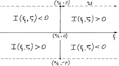
The symmetry relations presented in (42) imply that is symmetric with respect to the two perpendicular lines and in the plane . Similarly, is symmetric with respect to point and skew-symmetric with respect to the lines and .
Step 2. Because of the symmetry, without loss of generality, we may assume that , which is the upper-right quadrant. Now we are ready to solve the equation . First we need to describe all solutions for the real parts of this equation, i.e., . Let us define two quadrants , and the level set by
| (43) |
It is clear that is the closure of . The following proposition describes all possible types of such level sets.
Proposition 3.2 (Level curves description).
-
1.
For every fixed the set of solutions for the equation
(44) is a continuous curve .
-
2.
The function is and for every point such that .
-
3.
No two of these curves have common points in .
Remark 3.3.
According to Theorem 6.1, ([4], p. 128), if a level curve starts at the corner , then it bisects the corner and if a level curve starts at the lower or at the left edge of , then it must be perpendicular to the edge. No two of these level curves have a common point in .
Proof of the Proposition 3.2.
First, we need to analyze the behavior of partial derivatives of in .
Claim 3.4.
| (45) |
Proof of the claim 3.4.
Note that is function of both variables and, according to (42), is symmetric with respect to as a function of for every . This implies that
| (46) |
Note also that according to (35), p. 35,
| (47) |
for every defined in (36). It is clear that (46) and (47) imply (45). This completes the proof of Claim 3.4. ∎
Claim 3.5.
| (48) |
Proof of the Claim 3.5.
Here we are going to use similar symmetry and second derivative arguments used in the proof of previous Claim. Recall that is function of both variables and, according to (42), is symmetric with respect to as a function of for every . This implies that
| (49) |
Note also that according to (35),
| (50) |
for every defined in (36), p. 36. It is clear that (49) and (50) imply (48). This completes the proof of Claim 3.5. ∎
For the next step we need the following notation for the boundary parts of . With every we associate two curves and as shown on the Figure 4 below and defined as follows.
| (51) |
| (52) |
Note then, according to (45) and (48), the value of is a continuous and strictly increasing function as the point runs along from to and
| (53) |
On the other hand, . Therefore, there exists the unique point such that .
Note also that by (48), is continuous and strictly decreasing along the vertical segment connecting and . Thus, . Then, when the point runs along from to , the value of is continuously and strictly increasing to , according to (45) and (47). Therefore, there exists the unique point such that . Clearly, .
Now we are ready to describe the level set for any fixed .
Claim 3.6.
| (54) |
Proof of the Claim 3.6.
Claim 3.7.
can be interpreted as the graph of a function , i.e.,
| (55) |
Proof.
Fix any . Then, for the vertical segment connecting two points and we can observe that
| (56) |
since, according to (45), the value of is a strictly increasing function along every horizontal line in . Note also that the value of , according to (48), is strictly decreasing for . Hence, there exists the unique value of , such that , which completes the proof of Claim 3.7. ∎
To complete the proof of Proposition 3.2, from p. 3.2, we need to study the functional properties of the function . First, let us observe that for every , since the value of , according to (45), is a strictly increasing function along the lower edge of . Therefore, by the Implicit Function Theorem, for every there exists some neighborhood , where is continuously differentiable times for any natural and then, according to (45) and (48), we have
| (57) |
A possible curve starting with the horizontal edge of is sketched on Figure 4, page 4. Note also that is continuous in , since is monotone in and is continuous in . Now the proof of the Proposition 3.2 from p. 3.2 is complete. ∎
Step 3. The goal of this step is to obtain the following proposition.
Proposition 3.8.
If , then the equation has the unique solution , i.e., .
Proof of the Corollary 3.8..
It is clear that a solution may appear only on the level curve described above. For a point to be a solution we need . So, let us study the behavior of along . By the direct computation we can observe that
| (58) |
which together with (57) leads to
| (59) |
for every , where the last inequality holds because of (48) from Claim 3.5, p. 3.5. Therefore, the value of is a strictly increasing function on and then, the function assumes each of its values for only once. Hence, the equation must have only one solution in . This completes the proof of the Proposition 3.8. ∎
Step 4. The next and the last stage in the proof of Statement (D) is to analyze the behavior of in
Proposition 3.9.
| (60) |
| (61) |
The signum of behavior is sketched on Figure 5 below.
Proof of Proposition 3.9..
Using the skew-symmetry of introduced in (42), p. 42, we can observe that
| (62) |
On the other hand, we can observe that the condition yields
| (63) |
for every value of , except and then, for every point , one of following relations depending on the signum of holds
| (64) |
which to together with (62) implies (60) and (61). This completes the proof of Proposition 3.9. ∎
∎
Proof of Corollary 2.6, p. 2.6..
Proof of Corollary 2.9 from p. 2.9..
Note that the condition: is sufficient to find and such that and the equalities hold. Note also that if we integrate a -periodic function over the period from 0 to , we can replace by and vice versa without changing the result of the integration. Thus, the function under the integral can be reduced to the Poisson kernel, which yields
Proof of Corollary 2.10 from p. 2.10..
We organize the proof as the chain of identities, which will be explained at each step.
- Step 1.
-
Using the Statement (A) from p. (A) and comparing imaginary parts for both integrals with and , we have
(71) - Step 2.
-
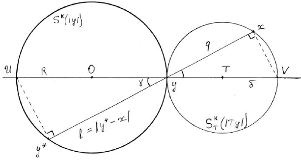
Let be the unit sphere centered at point . Then, we can observe that
(72) where all notations are pictured on the Figure 6 below that can be used for a reference. Thus, the last integral in (71) can be written as
(73) 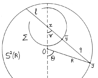
Figure 6: Reference picture. - Step 3.
- Step 4.
-
Observe that the last integrand is symmetric with respect to . Indeed, and
(76) where the symbol denotes composition. Hence, the integral in (75) can be written as
(77) - Step 5.
- Step 6.
-
The last integral can be computed directly and then the integral in (78) yields
(79) - Step 7.
The partial case stated in (16), p. 16 can be obtained by taking limit at both parts of (15) as . This limit exists since the integrand in (15), p. 15 or equivalently, in (71), p. 71 converges uniformly as . This completes the proof of Corollary 2.10, p. 2.10. ∎
4 Appendix
The main goal of this section is to use the ratio of two segments and defined above, to analyze the behavior of as approaches . We show that and depends on the path chosen for to approach .
Lemma 4.1.
Let be any point on the line such that and let be the sphere of radius centered at , where is the distance from to . Then
| (82) |
Proof of Lemma 4.1.
Let us choose as it is shown on Figure 7 below.
Let , and be the intersections of line with the spheres and respectively. is defined by the definition 2.1. Let . Observe that since the segments and are diameters. Therefore,
| (83) |
and
| (84) |
Hence, the combination of (3), (83) and (84) yields
| (85) |
Therefore, for the chosen point formula (82) is justified. A similar argument yields (82) for all other positions of on the line . This completes the proof of Lemma 4.1. ∎
Corollary 4.2.
Let be the path through and let . Then
| (86) |
where the value depends on the path chosen and can assume any value from the closed interval .
Proof of Corollary 4.2.
Note first, if , then for every and therefore, . If , then, by (82),
| (87) |
which can be any number from depending on chosen on the line . In particular, if , then , which corresponds to the case when belongs to the tangent hyperplane to at point . In this case for every . Finally, to get , must be a curve non-tangential to at point . Indeed, let be the angle between and line at point as it is pictured on Figure 8 below.
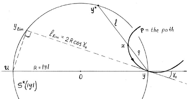
Note that is the diameter which implies that , and then,
| (88) |
while
| (89) |
Therefore,
| (90) |
which completes the proof of Corollary (4.2). ∎
References
- [1] H.A. Schwarz, Gesammelte Mathematische Abhandlungen, Chelsea Publishing Company Bronx, New York, 1972, (pp. 359-361).
- [2] Lars V. Ahlfors, Complex Analysis, McGraw-Hill, Inc., 1966, (pp. 168-169).
- [3] Reinhold Remmert, Classical Topics in Complex Function Theory, Springer-Verlag New York, Inc., 1998.
- [4] S.Artamoshin, Geometric Interpretation of the 2-D Poisson Kernel and Its Applications, http://arxiv.org/pdf/0912.0223v1.pdf, 2009.