Bethe-Heitler emission in BL Lacs: filling the gap between X-rays and $\gamma$-rays

Abstract

We present the spectral signatures of the Bethe-Heitler pair production ($pe$) process on the spectral energy distribution (SED) of blazars, in scenarios where the hard $\gamma$-ray emission is of photohadronic origin. If relativistic protons interact with the synchrotron blazar photons producing $\gamma$ rays through photopion processes, we show that, besides the $\sim 2-20$ PeV neutrino emission, the typical blazar SED should have an emission feature due to the synchrotron emission of $pe$ secondaries that bridges the gap betweeen the low-and high-energy humps of the SED, namely in the energy range $40$ keV – $40$ MeV. We first present analytical expressions for the photopion and $pe$ loss rates in terms of observable quantities of blazar emission. For the $pe$ loss rate in particular, we derive a new approximate analytical expression for the case of a power-law photon distribution, which has an excellent accuracy with the numerically calculated exact one, especially at energies above the threshold for pair production. We show that for typical blazar parameters, the photopair synchrotron emission emerges in the hard X-ray/soft $\gamma$-ray energy range with a characteristic spectral shape and non negligible flux, which may be even comparable to the hard $\gamma$-ray flux produced through photopion processes. We argue that the expected “$pe$ bumps” are a natural consequence of leptohadronic models, and as such, they may indicate that blazars with a three-hump SED are possible emitters of high-energy neutrinos.

1 Introduction

Blazars are a subclass of active galactic nuclei with a non-thermal continuum emission spanning many orders of magnitude in energy, i.e. from radio frequencies up to high-energy $\gamma$-rays. Their spectral energy distribution (SED) has a double humped appearance (e.g. Ulrich et al. 1997; Fossati et al. 1998) with a broad low-energy component extending from radio up to UV, or in some extreme cases to $\gtrsim 1$ keV X-rays (Costamante et al., 2001), and the high-energy one covering the X-ray and $\gamma$-ray energy regime with a peak energy around $0.1$ TeV, but this is not always clear (see e.g. Abdo et al. 2011b for Mrk 421). Although they exhibit variability in almost all frequencies (e.g. Raiteri et al. 2012), the rapid high-energy variability is one of their striking features. Variability timescales may range between $\sim$ day and several hours (Kataoka et al., 2001; Sobolewska et al., 2014), while in some extreme cases they may reach down to a few minutes in GeV and TeV energies (Aharonian et al., 2007; Aleksić et al., 2011; Foschini et al., 2013). Their variable emission when combined with the large inferred isotropic luminosities provides strong evidence that blazar emission originates in relativistic jets that are closely aligned with our line of sight.

It is generally accepted that the low-energy component is the result of synchrotron radiation from relativistic electrons in the jet, yet the origin of the high-energy component remains an open issue. Theoretical models for blazar emission are divided into leptonic and leptohadronic, according to the type of particles responsible for the high-energy emission. It is noteworthy that both have been successfully applied to blazars (for a review, see Böttcher 2010). In pure leptonic scenarios, the high-energy component is the result of inverse Compton scattering of electrons in a photon field. As seed photons can serve the synchrotron photons produced by the same electron population (SSC models: Maraschi et al. 1992; Bloom & Marscher 1996; Mastichiadis & Kirk 1997; Konopelko et al. 2003) or/and photons from an external region (EC models), such as the accretion disk (Dermer et al., 1992; Dermer & Schlickeiser, 1993) or the broad line region (BLR) (Sikora et al., 1994; Ghisellini & Madau, 1996; Böttcher & Dermer, 1998). EC models in particular, are more relevant for flat spectrum radio quasars (FSRQs) and/or low-peaked blazars (LBLs); for modelling of specific sources belonging to both classes, see Böttcher et al. (2013).

In principle, both protons and electrons can be accelerated to relativistic energies (Biermann & Strittmatter 1987; Sironi et al. 2013; Globus et al. 2014 and references, therein). This argument consists the basis of leptohadronic models, where the low-energy component of the SED is still explained by electron synchrotron radiation, but the high-energy emission is now explained in terms of relativistic proton interactions in the jet. Models that invoked interactions of relativistic protons with ambient matter (gas) through $pp$ collisions (e.g. Stecker et al. 1991; Beall & Bednarek 1999; Schuster et al. 2002) required high densities of the gas to explain the observed luminosities. Attention was then drawn to proton interactions with low energy photons (photohadronic interactions), since their density in astrophysical environments usually exceeds that of the gas. In these models, target photons may be provided either externally from the jet (same as in EC models), i.e. from the accretion disk (Bednarek & Protheroe, 1999) and the BLR (Atoyan & Dermer, 2001), or they can be internally produced by the co-accelerated electrons. The similarity to the SSC models is again obvious. The high-energy component can be the result of (i) the emission from an electromagnetic (EM) cascade initiated by the absorption of very high-energy (VHE) $\gamma$ rays produced through the $p\pi$ process (Mannheim et al., 1991; Mannheim & Biermann, 1992; Mannheim, 1993); (ii) synchrotron radiation of secondary pairs produced by the decays of charged pions (Petropoulou & Mastichiadis, 2012; Mastichiadis et al., 2013); (iii) neutral pion decay (Sahu et al., 2013; Cao & Wang, 2014); or proton synchrotron radiation, for high enough magnetic fields (Aharonian, 2000; Mücke & Protheroe, 2001; Mücke et al., 2003; Petropoulou, 2014b).

Photohadronic interactions are comprised of two processes of astrophysical interest:

• Bethe-Heitler pair production ($pe$)

  $$p+\gamma\rightarrow e^{+}+e^{-}.$$ (1)

• Photopion production ($p\pi$)

  $$p+\gamma \rightarrow \pi^{0}+p$$ (2)

  $$\pi^{0} \rightarrow \gamma+\gamma$$

  or

  $$p+\gamma \rightarrow \pi^{\pm}+n\left(\Delta^{++}\right),$$ (3)

  $$\pi^{\pm} \rightarrow \mu^{\pm}+\nu_{\mu}(\overline{\nu}_{\mu}),$$

  $$\mu^{\pm} \rightarrow e^{\pm}+\overline{\nu}_{\mu}(\nu_{\mu})+\nu_{\rm e}(\overline{\nu}_{\rm e}).$$

Bethe-Heitler pair production is an often overlooked process since it is not related with neutrino and neutron production, which is of particular interest to high-energy astrophysics and a natural outcome of $p\pi$ interactions (Sikora et al., 1987; Kirk & Mastichiadis, 1989; Begelman et al., 1990; Giovanoni & Kazanas, 1990; Waxman & Bahcall, 1997; Atoyan & Dermer, 2001, 2003). Moreover, it is considered to be a subdominant proton cooling process, at least for protons that satisfy the threshold condition for $p\pi$ production (e.g. Sikora et al. 1987) and thus, is often neglected in models of blazar emission (e.g. Cerruti et al. 2011; Böttcher et al. 2013; Weidinger & Spanier 2013). However, as we shall show in the present study, $pe$ secondaries are injected at different energies than photopion ones. Therefore, even in cases where $pe$ is subdominant, it can still leave a radiative signature on the blazar spectrum. An illustration of the $pe$ contribution to the injection of secondaries can be found in Fig. 8 of Dimitrakoudis et al. (2012)–henceforth DMPR12, and Petropoulou (2014a).

The aim of the present work is to study in more detail the contribution of pairs injected by the $pe$ process to the SED of blazars. We focus on BL Lac objects, a subclass of blazars named after the prototype object BL Lacartae (Schmitt, 1968) because of two reasons: the majority of BL Lac objects is detected in high-energy $\gamma$ rays ($\gtrsim 100$ GeV) and is characterized by an extreme weakness of emission lines in the optical spectra, which suggests that any external radiation fields play a subdominant role in the formation of their spectra. BL Lacs, as less “contaminated” sources than FSRQs, consistute a more suitable class of objects for studying the emission signatures of photohadronic interactions. The role of the $pe$ process in the emission of FSRQs will be the subject of a future work.

The theoretical framework that we adopt is described as follows: the low-energy emission is explained by synchrotron radiation of relativistic electrons, whereas the observed high-energy (GeV-TeV) emission is the result of synchrotron radiation from pairs produced by charged pion decays. Pions in their turn, are the by-product of $p\pi$ interactions of co-accelerated protons with the internally produced synchrotron photons. We restrict our analysis to cases where the high-energy spectra are not (severely) modified by EM cascades, which allows us to identify the observed $\gamma$-ray emission as the emission from the $p\pi$ component. Thus, in this framework, the $\gamma$-ray blazar emission is directly associated with neutrino emission at energies $\sim 2-20$ PeV, which may be of particular interest in the light of the recent detection of astrophysical high-energy neutrinos (IceCube Collaboration, 2013; Aartsen et al., 2014).

Our work is structured as follows. We begin in §2 with a description of our model. In §3 we derive analytical expressions for the typical energies of synchrotron photons emitted by secondary pairs produced through the $pe$ and $p\pi$ processes, and compare the respective proton cooling rates for typical blazar parameters. In §4 we back up our analytical predictions with numerical examples. We discuss our results in §5 and conclude in §6 with a summary.

2 The model

We assume that the region responsible for the blazar emission can be described as a spherical blob of size $r_{\rm b}$ that contains a tangled magnetic field of strength $B$, moving with a Doppler factor $\delta=\Gamma^{-1}\left(1-\beta\cos\theta\right)^{-1}$, where $\Gamma$ is the bulk Lorentz factor and $\theta$ is the angle between the line of sight and the jet axis. We also assume that both protons and primary electrons are injected uniformely with a constant rate into the emission region, after having been accelerated to relativistic energies; their distribution is described by a power-law with index $s_{i}$ and high-energy cutoff $\gamma_{\rm i,\max}$, where the subscript $i$ is used to discriminate between protons ($p$) and electrons ($e$). Electrons lose energy through the synchrotron and inverse Compton processes, while synchrotron radiation and photohadronic interactions count to the main energy loss processes for relativistic protons. In the present context, we assume that the target photons for the photohadronic interactions, which include both $pe$ and photopion production processes, are internally (or locally) produced, i.e. they are the result of primary electron (and proton) synchrotron radiation. Photohadronic interactions eventually lead to an increase of the lepton number density in the emission region, since both $pe$ and $p\pi$ processes result in the injection of secondary pairs. Thus, synchrotron and inverse Compton radiation of secondary pairs is an inevitable outcome of photohadronic interactions, which, depending on the parameters, may be imprinted on the blazar SED.

In the present work we investigate a typical leptohadronic scenario that relates the observed blazar $\gamma$-ray emission with a high-energy neutrino signal. In this context, the synchrotron emission from primary electrons and from the $p\pi$ process contributes to the low and the high parts of the spectrum respectively. On the other hand, the $pe$ process typically injects pairs with lower energy than the $p\pi$ secondaries, and we thus expect their synchrotron radiation to emerge between the two spectral humps. This is exemplified in Fig. 1 where a fiducial blazar SED is shown schematically. Besides the low-and high-energy humps (black lines), the contribution of the $pe$ pairs to the SED is shown as a third component (red line) that emerges between the two (grey colored region). We argue that the $pe$ emission that bridges the two humps of the SED is a robust prediction of this model. In the following sections we investigate this argument in detail using both analytical and numerical means.

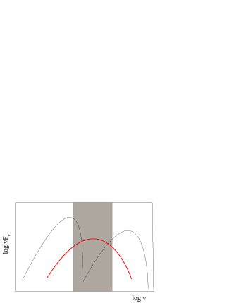
Figure 1: Sketch of a typical blazar SED in $\nu F_{\nu}$ units with the low and high energy humps shown with black lines. Synchrotron emission from Bethe-Heitler pairs is expected to appear as a third bump (red line) in the hard X-ray/soft $\gamma$-ray regime (grey colored zone).

3 Analytical estimates

When one fixes the primary electron and proton population so they can explain the characteristic double humps observed in blazars, then the $pe$ component is determined automatically without the use of any additional parameter. We present analytical expressions for the typical synchrotron photon energies emitted by secondary $pe$ and $p\pi$ pairs, which we express in terms of observable quantities of blazar emission. We continue with the calculation of the $pe$ and photopion energy loss rates for monoenergetic and power-law target photon fields, and compare them for parameter values typical for blazar emission. We note that the analysis that follows is valid as long as the photon spectra are not modified by electromagnetic cascades initiated by internal photon-photon absorption (see e.g. Mannheim et al. 1991).

3.1 Characteristic energies

We estimate the characteristic energies of synchrotron photons emitted by secondary electrons, which are the products of $pe$ pair production and charged pion decay, and express them using observable quantities, such as the peak frequencies of the low-and high-energy humps of the blazar SED. We list below the basic relations we used and note that primed variables denote quantities measured in the comoving frame of the region, whereas unprimed variables are used for quantities measured in the observer’s frame:

1. The low-energy bump of the SED is explained in terms of primary electron synchrotron radiation. Its peak frequency $\nu_{\rm s}$ is then written as $\nu_{\rm s}=\delta(1+z)^{-1}h^{-1}(B/B_{\rm cr})m_{\rm e}c^{2}\gamma_{e}^{2}$, where $z$ is the redshift of the source, $B_{\rm cr}=4.4\times 10^{13}$ G and $\gamma_{e}$ is the Lorentz factor of primary injected electrons. Using $10^{16}$ Hz as a typical value for the peak frequency we derive the first relation

   $$\delta B\gamma_{e}^{2}=3.5\times 10^{9}\nu_{\rm s,16}.$$ (4)

2. The proton threshold energy for $p\pi$ interactions with the synchrotron photons of energy $\epsilon^{\prime}_{\rm s}=h\nu_{\rm s}(1+z)/\delta$ is given by

   $$\gamma_{\rm p,p\pi}^{\rm(th)}\simeq\frac{x_{\rm th}}{x_{\rm s}},$$ (5)

   where $x_{\rm th}=m_{\pi}/m_{\rm e}$ for single pion production, $m_{\pi}\simeq 145$ MeV/$c^{2}$ and $x_{\rm s}=\epsilon^{\prime}_{\rm s}/m_{\rm e}c^{2}$ or

   $$x_{\rm s}=8\times 10^{-5}(1+z)\nu_{\rm s,16}\delta^{-1},$$ (6)

   in terms of the obsverved peak frequency. Inserting the above expression into eq. (5) we find

   $$\gamma_{\rm p,p\pi}^{\rm(th)}\simeq 3.5\times 10^{6}(1+z)^{-1}\delta\nu_{\rm s,16}^{-1}.$$ (7)

3. The proton threshold energy for $pe$ pair production on synchrotron photons of energy $\epsilon^{\prime}_{\rm s}$ is given by

   $$\gamma_{\rm p,pe}^{\rm(th)}\simeq 1.2\times 10^{4}(1+z)^{-1}\delta\nu_{\rm s,16}^{-1},$$ (8)

   which is lower than the respective one for pion production by a factor of $m_{\rm e}/m_{\pi}$.

4. We assume that the secondary electrons produced through $p\pi$ interactions from parent protons having energy $\gamma_{\rm p,p\pi}^{\rm(th)}$ emit synchrotron radiation at high-energy $\gamma$ rays, e.g. $\nu_{\gamma}\gtrsim 10^{25}$ Hz. The secondary electrons are produced roughly with a Lorentz factor $\gamma_{\rm e}^{p\pi}\simeq\kappa_{\rm p}\gamma_{\rm p,p\pi}^{\rm(th)}m_{\rm p}/4m_{\rm e}$, where $\kappa_{\rm p}\simeq 0.2$ is the mean inelasticity of $p\pi$ interactions. Using eq. (7) we find the constraint

   $$\delta^{3}B\simeq 30(1+z)^{3}\nu_{\rm s,16}^{2}\nu_{\gamma,25}.$$ (9)

Finally, the typical Lorentz factor of primary electrons is derived by combining eqs. (4) and (9)

$$\gamma_{\rm e}\simeq 10^{3}\delta(1+z)^{-1}\left(\nu_{\rm s,16}\nu_{\gamma,25}\right)^{-1/2}.$$ (10)

Before continuing to the calculation of the proton energy loss rates due to photohadronic processes, it is useful to have an estimate of the energy range where the synchrotron emission from $pe$ pairs emerges.

For proton-photon collisions taking place close to the threshold, the maximum Lorentz factor of the produced pairs is $\gamma_{\rm e}^{\rm pe}\approx\gamma_{\rm p}$ (Mastichiadis & Kirk, 1995; Kelner & Aharonian, 2008). Using the expressions (8) and (9) we find

$$\nu_{\rm s}^{\rm pe}\simeq 5.2\times 10^{16}\nu_{\gamma,25}\ {\rm Hz},$$ (11)

which falls in the UV/soft X-ray energy band. However, $pe$ emission at these energies should not have any observable effect on the SED, since the injection rate of $pe$ pairs close to the threshold is small. This is a direct outcome of the fact that the product of the $pe$ cross section and proton inelasticity has its maximum at $\gamma_{\rm p}x\approx 16$, where $x$ is the energy of an arbitrary photon in $m_{\rm e}c^{2}$ units (see e.g. Fig. 1 in Mastichiadis et al. 2005). For a power-law proton distribution, which is the case under consideration here, protons with energies above the photopair threshold, i.e. $\gamma_{\rm p}\gtrsim\gamma_{\rm p,pe}^{\rm(th)}$, will also interact with photons of energy $\epsilon^{\prime}_{\rm s}$. In this case, however, the interactions occur away from the threshold. For $\bar{\epsilon}=2\gamma_{\rm p}\epsilon^{\prime}_{\rm s}\gg m_{\rm e}c^{2}$, where $\bar{\epsilon}$ is the energy of the synchrotron photons as measured in the proton’s rest frame, the pairs acquire a higher maximum Lorentz factor given by $\gamma_{\rm e}^{\rm pe}\approx 4\gamma_{\rm p}^{2}x_{\rm s}\gtrsim 4\left(\gamma_{\rm p,pe}^{\rm(th)}\right)^{2}x_{\rm s}$ (Kelner & Aharonian, 2008). Using eqs. (6), (8) and (9) we find that

$$\nu_{\rm s}^{\rm pe}\gtrsim 3.3\times 10^{18}\nu_{\gamma,25}\ {\rm Hz},$$ (12)

which corresponds to the hard X-ray/soft $\gamma$-ray regime, where the emission from $pe$ pairs is expected to have its peak. We shall show this in §4 with numerical examples that take into account the exact injection distribution of $pe$ pairs. Concluding, expressions (11) and (12) indicate that the synchrotron emission from $pe$ pairs spans over a wide range of energies (see also Fig. 4 in DMPR12), and may contribute to the soft $\gamma$-ray emission affecting therefore the spectral shape of the SED.

3.2 Proton energy loss rates

The proton energy loss rate due to the $i$ process is defined as $t_{\rm i}^{-1}=-(d\gamma_{\rm p}/dt)_{\rm i}\gamma_{\rm p}^{-1}$. The energy loss timescale due to $p\pi$ interactions is given by (Stecker 1968; Begelman et al. 1990– henceforth, BSR90):

$$t_{\rm p\pi}^{-1}\left(\gamma_{\rm p}\right)=\frac{c}{2\gamma_{\rm p}^{2}}\int_{\bar{\epsilon_{\rm th}}}^{\infty}d\bar{\epsilon}\sigma_{p\pi}(\bar{\epsilon})\kappa_{\rm p}(\bar{\epsilon})\bar{\epsilon}\int_{\bar{\epsilon}/2\gamma_{\rm p}}^{\infty}d\epsilon^{\prime}\frac{n^{\prime}(\epsilon^{\prime})}{\epsilon^{{}^{\prime}2}},$$ (13)

where bared quantities are measured in the proton’s rest frame, $\bar{\epsilon}_{\rm th}=145$ MeV, $\sigma_{p\pi}$ and $\kappa_{\rm p}$ are the cross section and proton inelasticity, respectively, and $n^{\prime}(\epsilon^{\prime})$ is the photon number density in the comoving frame of the emission region. Above the threshold for $p\pi$ production the cross section is dominated by the $\Delta$(1232) resonance ($\sigma_{p\pi}\simeq 0.5$ mb). Various other resonances, albeit less important than the $\Delta(1232)$ resonance, shape the cross section up to $\bar{\epsilon}\sim 1$ GeV. At higher energies though, the cross section becomes approximately energy independent with a value $\sim 0.1$mb (Mücke et al., 2000; Beringer et al., 2012). The two-step function approximation of $\sigma_{p\pi}$ presented in Atoyan & Dermer (2001) is an elaborate choice, which also takes into account the increase of the proton inelasticity as the interactions occur away from the threshold. However, since the exact numerical value of the proton loss rate is not central in our case, we adopt the more crude, yet simpler, approximation $\sigma_{p\pi}\approx\sigma_{0}H(\bar{\epsilon}-\bar{\epsilon}_{\rm th})$ with $\sigma_{0}\approx 1.5\times 10^{-4}\sigma_{\rm T}$ (see also Petropoulou & Mastichiadis 2012), and a constant inelasticity $\kappa_{\rm p}=0.2$.

The proton energy loss rate for the $pe$ process on an isotropic photon field was derived by Blumenthal (1970) – henceforth B70, and is given by

$$t_{pe}^{-1}\left(\gamma_{\rm p}\right)=\frac{3}{8\pi\gamma_{\rm p}}\sigma_{\rm T}c\alpha_{\rm f}\frac{m_{\rm e}}{m_{\rm p}}\int_{2}^{\infty}d\kappa\ n^{\prime}\left(\frac{\kappa}{2\gamma_{\rm p}}\right)\frac{\phi(\kappa)}{\kappa^{2}},$$ (14)

where $\alpha_{\rm f}$ is the fine structure constant, $\kappa=2\gamma_{\rm p}\epsilon^{\prime}/m_{\rm e}c^{2}$, and $\phi(\kappa)$ is a function defined by a double integral (see eq. (3.12) in Chodorowski et al. 1992; henceforth CZS92). CZS92 derived analytical approximate expressions for $\phi(\kappa)$, yet the analytical calculation of the integral in eq. (14) is cumbersome even for the case of a power-law photon distribution (see appendix).

For BL Lac objects, the main contribution to $n^{\prime}(\epsilon^{\prime})$ comes from the synchrotron radiation of primary electrons. We express the photon number density in terms of observable quantities, such as the bolometric synchrotron luminosity $L_{\rm syn}$. The energy density of synchrotron photons in the comoving frame is given by

$$u^{\prime}_{\rm syn}\approx\frac{3L_{\rm syn}}{4\pi\delta^{4}r_{\rm b}^{2}c},$$ (15)

where $r_{\rm b}$ is the comoving size of the emission region. In the limit of $\theta\lesssim 1/\Gamma$ and $\Gamma\gg 1$, we find $\delta\approx\Gamma$. From this point on, we will use interchangeably $\delta$ and $\Gamma$. The low-energy spectrum of blazars, especially that of LBLs, can often be described by a steep power-law for energies above its peak in $\epsilon L(\epsilon)$ units. For indicative examples, see Fig. 2 in Ghisellini (2001) and Fig. 5 in Böttcher et al. (2013). For this reason, we derive explicit expressions of $t_{\rm p\pi}^{-1}$ and $t_{pe}^{-1}$ for a power-law synchrotron photon distribution. As a first step though, and for completeness reasons, we examine the case of a monoenergetic photon distribution. This can be considered as a zero order approximation for a narrow (in energy) low-energy hump, and faciliates the derivation of simple analytic relations.

3.2.1 Monoenergetic photon distribution

We assume that the synchrotron photon field is monoenergetic with energy $\epsilon_{\rm s}$. The differential photon number density in the comoving frame is then written as

$$n^{\prime}(\epsilon^{\prime})=n^{\prime}_{0}\epsilon^{\prime}\delta(\epsilon^{\prime}-\epsilon^{\prime}_{\rm s}),$$ (16)

with $n^{\prime}_{0}=u^{\prime}_{\rm syn}/\epsilon_{\rm s}^{{}^{\prime}2}$. We note that the rectangular approximation of the $p\pi$ cross section, which is adequate for the case of power-law photon distributions (e.g. Murase et al. 2014), is not appropriate in this case, since it understimates the cooling of protons with energies much above the threshold. Using eqs. (13) and (16) we find the energy loss rate to be

$$t_{\rm p\pi}^{-1}\left(\xi_{p\pi}\right)\approx 7\times 10^{-5}\ s^{-1}\left(1-\frac{1}{\xi_{p\pi}^{2}}\right)\frac{L_{\rm syn,45}}{r^{2}_{\rm b,15}\delta^{3}\nu_{\rm s,16}\left(1+z\right)},\ \xi_{p\pi}>1,$$ (17)

where $\xi_{p\pi}=2\gamma_{\rm p}/\gamma_{\rm p,p\pi}^{\rm(th)}$. The dimensionless energy loss rate is defined as $t_{\rm p\pi}^{-1}/t_{\rm cr}^{-1}$, where $t_{\rm cr}=r_{\rm b}/c$ and is also an efficiency measure of the process. This is written as

$$f_{\rm p\pi}(\xi_{p\pi})\approx 2.2\left(1-\frac{1}{\xi_{p\pi}^{2}}\right)\frac{L_{\rm syn,45}}{r_{\rm b,15}\delta^{3}\nu_{\rm s,16}\left(1+z\right)},\ \xi_{p\pi}>1.$$ (18)

The loss rate becomes constant for $\gamma_{\rm p}$ slightly above the threshold, which is in rough agreement with numerical calculations where the full cross section and the energy-dependent inelasticity are used.

Subtitution of eq. (16) into eq. (14) leads to

$$t_{pe}^{-1}(\gamma_{\rm p}) = \frac{3}{8\pi}\sigma_{\rm T}c\alpha_{\rm f}\frac{m_{\rm e}}{m_{\rm p}}n^{\prime}_{0}m_{\rm e}c^{2}\frac{\phi\left(2\gamma_{\rm p}x_{\rm s}\right)}{2\gamma_{\rm p}^{2}x_{\rm s}},\ \gamma_{\rm p}>\frac{1}{x_{\rm s}}$$ (19)

$$t_{pe}^{-1}(\xi_{\rm pe}) \simeq 2\times 10^{-6}\ s^{-1}\ g(\xi_{\rm pe})\frac{L_{\rm syn,45}}{r^{2}_{\rm b,15}\delta^{3}\nu_{\rm s,16}\left(1+z\right)},\xi_{\rm pe}>1,$$ (20)

where $\xi_{\rm pe}=2\gamma_{\rm p}/\gamma_{\rm p,pe}^{\rm(th)}$ with $\gamma_{\rm p,pe}^{\rm(th)}$ given by eq. (8) and $g(\xi)=\phi(\xi)/\xi^{2}$, which has its maximum $g_{\max}\sim 1$ at $\xi\simeq 47$ (see Fig. 2 in CZS92). Similarly to the $p\pi$ efficiency, for the $pe$ process we find

$$f_{pe}(\xi_{\rm pe})\approx 0.06g(\xi_{\rm pe})\frac{L_{\rm syn,45}}{r_{\rm b,15}\delta^{2}\nu_{\rm s,16}\left(1+z\right)},\xi_{\rm pe}>1.$$ (21)

As the dependence on the parameters related to blazar emission is the same in eqs. (18) and (21), we find that $f_{pe}\ll f_{\rm p\pi}$ for $\gamma_{\rm p}\geq\gamma_{\rm p,p\pi}^{\rm(th)}$ in the case of monoenergetic photons.

3.2.2 Power-law photon distribution

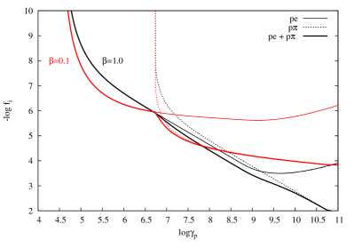
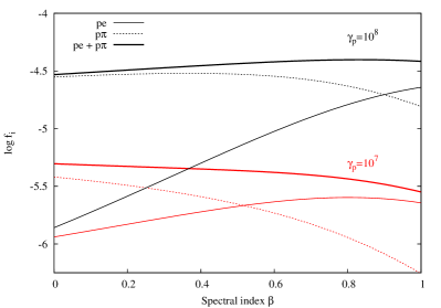
Figure 2: Left panel: Logarithmic plot of the dimensionless loss timescales $f_{pe}^{-1}$ (thin solid lines), $f_{\rm p\pi}^{-1}$ (dotted lines), and $f_{\rm p\pi}^{-1}+f_{pe}^{-1}$ (thick solid lines) as a function of $\gamma_{\rm p}$ for two spectral indices $\beta$ of the photon distribution marked on the plot. Right panel: Plot of the dimensionless loss rates $f_{pe}$ (thin solid lines), $f_{\rm p\pi}$ (dashed lines), and $f_{\rm p\pi}+f_{pe}$ (thick solid lines) as a function $\beta$ for $\gamma_{\rm p}=10^{7}$ (red lines) and $\gamma_{\rm p}=10^{8}$ (black lines). Other parameters used in both panels: $L_{\rm syn}=10^{45}$ erg/s, $r_{\rm b}=10^{15}$ cm, $\nu_{\rm s}=10^{17}$ Hz, $\epsilon_{\min}=10^{-4}\epsilon_{\max}$, $\epsilon_{\rm s}=\epsilon_{\max}$ and $\delta=30$.

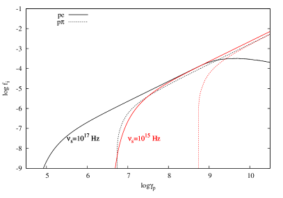
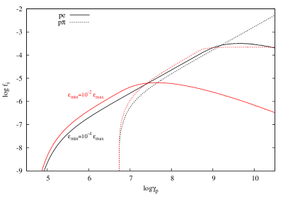
Figure 3: Logarithmic plots of the dimensionless loss rates $f_{pe}$ (solid lines) and $f_{\rm p\pi}$ (dotted lines) as a function of $\gamma_{\rm p}$. Left panel: Dependence on the high cutoff energy of the synchrotron spectrum for $\epsilon_{\min}=10^{-4}\epsilon_{\max}$. Black and red lines correspond to $\nu_{\rm s}=10^{17}$ Hz and $\nu_{\rm s}=10^{15}$ Hz, respectively. Right panel: Dependence on the low cutoff energy of the synchrotron spectrum for $\nu_{\rm s}=10^{17}$ Hz. Black and red lines correspond to $\epsilon_{\min}/\epsilon_{\rm s}=10^{-4}$ and $10^{-2}$, respectively. Other parameters used are: $L_{\rm syn}=10^{45}$ erg/s, $r_{\rm b}=10^{15}$ cm, $\delta=30$, $\beta=1$ and $\epsilon_{\rm s}\equiv\epsilon_{\max}$.

We assume that the differential luminosity scales as $L_{\rm syn}(\epsilon)\propto\epsilon^{-\beta}$ with $\beta>0$ for $\epsilon_{\min}<\epsilon<\epsilon_{\max}$, and normalize $L_{\rm syn}(\epsilon)$ with respect to the peak energy $\epsilon_{\rm s}=h\nu_{\rm s}$ (see point (i) in §3.1), which is set equal to $\epsilon_{\max}$ for $\beta\leq 1$ or $\epsilon_{\min}$ otherwise. Given that

$$L_{\rm syn}(\epsilon)=\frac{L_{0}}{\epsilon_{\rm s}}\left(\frac{\epsilon}{\epsilon_{\rm s}}\right)^{-\beta}$$ (22)

with the normalization $L_{0}$ being

$$\frac{L_{0}(\beta,\epsilon^{\prime}_{\rm s})}{L_{\rm syn}}=\left\{\begin{array}[]{cc}(1-\beta)\left(\frac{\epsilon_{\rm s}}{\epsilon_{\max}}\right)^{-\beta+1}\left[1-\left(\frac{\epsilon_{\min}}{\epsilon_{\max}}\right)^{-\beta+1}\right]^{-1},&\beta\neq 1\\ &\\ 1/\ln\left(\frac{\epsilon_{\max}}{\epsilon_{\min}}\right),&\beta=1,\end{array}\right.$$ (26)

we may write the differential photon number density in the comoving frame as

$$n^{\prime}(\epsilon^{\prime})=n^{\prime}_{0}\left(\frac{\epsilon^{\prime}}{\epsilon^{\prime}_{\rm s}}\right)^{-\beta-1}.$$ (27)

The respective normalization is

$$n^{\prime}_{0}=\frac{3L_{0}(\beta,\epsilon^{\prime}_{\rm s})}{4\pi c\delta^{4}r_{\rm b}^{2}\epsilon_{\rm s}^{{}^{\prime}2}}.$$ (28)

By inserting expression (27) into eq. (13) we calculate $t_{\rm p\pi}^{-1}$, which is now written as

$$t_{\rm p\pi}^{-1}(\gamma_{\rm p})=\frac{3L_{\rm syn}\lambda(\beta,\epsilon_{\rm s})\kappa_{\rm p}\sigma_{0}}{2\pi r_{\rm b}^{2}\delta^{3}\epsilon_{\rm s}(1+z)}\left\{\begin{array}[]{cc}\left(\frac{2\gamma_{\rm p}\epsilon^{\prime}_{\rm s}}{\overline{\epsilon}_{\rm th}}\right)^{\beta}-\left(\frac{\epsilon^{\prime}_{\rm s}}{\epsilon^{\prime}_{\max}}\right)^{\beta},&\gamma_{\rm p}<\frac{\bar{\epsilon}_{\rm th}}{2\epsilon^{\prime}_{\min}}\\ &\\ \left(\frac{\epsilon_{\rm s}}{\epsilon_{\min}}\right)^{\beta}&\gamma_{\rm p}>\frac{\bar{\epsilon}_{\rm th}}{2\epsilon^{\prime}_{\min}},\\ \end{array}\right.$$ (32)

where we neglected the contribution of the upper cutoff when performing the integral over the photon energies $\epsilon^{\prime}$. We also define $\lambda$ as

$$\lambda(\beta,\epsilon_{\rm s})=\frac{L_{0}(\beta,\epsilon^{\prime}_{\rm s})}{\beta(\beta+2)L_{\rm syn}},\ \beta\neq 0,-2.$$ (33)

We note that the first branch of eq. (32) coincides with eq. (5) in Mannheim et al. (1991) after making the replacements $2n^{\prime}_{0}(\epsilon^{\prime}_{\rm s})^{\beta+1}\rightarrow m_{0}$, $\beta\rightarrow\alpha_{\rm t}$, $\sigma_{0}\kappa_{\rm p}\rightarrow\langle\kappa\sigma_{\rm p\gamma\rightarrow\Delta}\rangle$, and for $\gamma_{\rm p}\gtrsim\gamma_{\rm p,p\pi}^{\rm(th)}\epsilon_{\rm s}/2\epsilon_{\max}$. It agrees also with the expression derived by eq. (4) in BSR90 for $\sigma^{\pi}(x^{\prime})K^{\pi}(x^{\prime})\approx\overline{\sigma^{\pi}(x^{\prime})K^{\pi}(x^{\prime})}$, where the latter corresponds to the product $\sigma_{0}\kappa_{\rm p}$ in this work. Since BSR90 assumed that the power-law photon distribution extends to very low energies, as to establish $\gamma_{\rm p}\epsilon^{\prime}_{\min}\lesssim\bar{\epsilon}_{\rm th}$, the second branch of eq. (32) was not relevant in their analysis.

In terms of the variable $\xi_{p\pi}$ the photopion efficiency is written as

$$f_{\rm p\pi}(\xi_{p\pi})\simeq 4.4\frac{L_{\rm syn,45}\lambda(\beta,\epsilon_{\rm s})}{r_{\rm b,15}\delta^{3}\nu_{\rm s,16}(1+z)}\left\{\begin{array}[]{cc}\xi_{p\pi}^{\beta},&\xi_{p\pi}<\frac{\epsilon_{\rm s}}{\epsilon_{\min}}\\ &\\ \left(\frac{\epsilon_{\rm s}}{\epsilon_{\min}}\right)^{\beta},&\xi_{p\pi}>\frac{\epsilon_{\rm s}}{\epsilon_{\min}}\\ \end{array}\right.$$ (37)

We neglected the term $\left(\epsilon^{\prime}_{\rm s}/\epsilon^{\prime}_{\max}\right)^{\beta}$ from the first branch of eq. (37) since it is always less than unity and we are interested in $\xi_{p\pi}\gtrsim 1$.

We found that a similar expression for the photopair production can also be derived, if the function $\phi(\kappa)/\kappa^{2}$ that appears in the integral of eq. (14) is approximated by a bi-Gaussian function with respect to $\ln\kappa$ (see appendix for more details). The dimensionless loss rate may be written as:

$$f_{pe}(\xi_{\rm pe})\simeq 0.06\ \frac{L_{\rm syn,45}\beta(\beta+2)\lambda(\beta,\epsilon_{\rm s})}{r_{\rm b,15}\delta^{3}\nu_{\rm s,16}(1+z)}\xi_{\rm pe}^{\beta}I(\gamma_{\rm p},\beta),$$ (38)

where $I(\gamma_{\rm p},\beta)$ is a function that may be expressed in terms of error functions. Although general use of eq. (38) may be cumbersome because of the presence of error functions, it can be used for having a first estimate of the $pe$ loss rate in the case of a power-law photon distribution. It also faciliates the comparison between the loss rates for the two channels of photohadronic interactions, since the expressions of eqs. (37) and (38) are similar, apart from the factor $I(\gamma_{\rm p},\beta)$. The ratio of the loss rates for a fixed proton energy is $f_{\rm p\pi}(\gamma_{\rm p})/f_{pe}(\gamma_{\rm p})\approx 73[(\beta+2)\beta]^{-1}\left(\gamma_{\rm p,pe}^{\rm(th)}/\gamma_{\rm p,p\pi}^{\rm(th)}\right)^{\beta}I(\gamma_{\rm p},\beta)^{-1}$. The ratio of the two rates becomes of order unity for $\beta\sim 1$ (see also BRS90), where we also used the fact that $I(\gamma_{\rm p},1)\sim 0.1$ for a wide range of $\gamma_{\rm p}$ values (see Fig. A3 in appendix).

In what follows, we numerically integrate eqs. (13) and (14) for a power-law photon distribution and compare the derived $f_{\rm p\pi}$ and $f_{pe}$ for different blazar parameters. The results are summarized in Figs. 2 and 3.

In general, we find that

• below the threshold energy for photopion production, proton losses are dominated by photopair production as expected (e.g. Stanev et al. 2000, DMPR12).

• in general, $p\pi$ losses dominate above the respective energy threshold but there are parameters leading to similar, at least within the same order of magnitude, energy loss rates. For example, we find $\eta=f_{pe}/f_{\rm p\pi}\sim 0.1-1$, for $\gamma_{\rm p}\gtrsim\gamma_{\rm p,p\pi}^{\rm(th)}$ and $\gamma_{\rm p}\gg\gamma_{\rm p,pe}^{\rm(th)}$ (left panel in Figs. 2 and 3).

• softer synchrotron spectra, namely larger $\beta$, favour $pe$ pair production, as shown in the right panel of Fig. 2.

• wider synchrotron spectra, i.e. larger value of the ratio $\epsilon_{\rm s}/\epsilon_{\min}$, favours also the $pe$ process (right panel in Fig. 3).

• higher peak frequencies push the threshold Lorentz factors to lower values, as eqs. (7) and (8) show. Thus, for a fixed proton energy much above the threshold for $pe$ pair production , higher $\nu_{\rm s}$ translates to lower $f_{pe}$; this can be seen in the left panel of Fig. 3.

• smaller values of the Doppler factor result in: an increase of both $f_{pe}$ and $f_{\rm p\pi}$ (see e.g. eqs. (37) and (38)) and a decrease of the respective threshold Lorentz factors (see eqs. (7) and (8)).

3.3 Luminosity estimates

If $L_{p\pi}$ and $L_{\rm pe}$ denote the bolometric synchrotron luminosities from pairs produced by the photopion and photopair processes, respectively, and under the assumption of efficient cooling of pairs, we may write $L_{\rm pe}\approx f_{pe}L_{\rm p}$ and $L_{p\pi}\approx(f_{\rm p\pi}/8)L_{\rm p}$, where $L_{\rm p}$ is the proton luminosity. The latter is derived under the assumptions that approximately half of the produced pions are neutral, thus not contributing to the injection of pairs, and that the produced electron/positron acquires $\sim 1/4$ of the proton’s energy in each $p\pi$ collision. The luminosity ratio of the two components is then given by $L_{\rm pe}/L_{p\pi}\approx 8\eta$. If we combine this estimate with the fact that the typical energy of synchrotron photons emitted by the $pe$ pairs for $\gamma_{\rm p}\gg\gamma_{\rm p,pe}^{\rm(th)}$ falls in the hard X-ray/soft $\gamma$-ray energy range (see §3.1), we expect a third bump in the SED with luminosity $\sim 8\eta$ of the $\gamma$-ray luminosity. Thus, for parameters that lead to $\eta\sim 0.1-1$ the additional component has the same order of magnitude luminosity with the $\gamma$-rays. Interestingly, even if $\eta\ll 1$, we expect that the $pe$ emission can still bridge the two main humps of the SED, since the synchrotron emission from $pe$ pairs does not, in general, overlap with the one from $p\pi$ produced pairs (see e.g. Fig. 1).

Going one step further, we may relate $L_{\rm pe}$ with the luminosity emitted in neutrinos, which are a by-product of $p\pi$ interactions. Let us first estimate what is the typical neutrino energy, which in $m_{\rm e}c^{2}$ units and in the comoving frame is written as

$$x_{\nu}\approx\frac{1}{4}\kappa_{\rm p}\gamma_{\rm p}\frac{m_{\rm p}}{m_{\rm e}}.$$ (39)

For protons with $\gamma_{\rm p}=\gamma_{\rm p,p\pi}^{\rm(th)}$ this translates to an observed energy

$$\epsilon_{\nu}^{\rm(th)}\simeq 0.2\ {\rm PeV}\ \delta^{2}(1+z)^{-2}\nu_{\rm s,16}^{-1},$$ (40)

where we used eq. (7) and the superscript ‘th’ is used as reminder for the parent proton’s energy. The ratio $\mathcal{R}_{\nu,\gamma}$ of the typical neutrino ($x_{\nu}$) and synchrotron photon energies from $p\pi$ pairs ($x_{\rm s}^{p\pi}$) is given by

$$\mathcal{R}_{\nu,\gamma}\equiv\frac{x_{\nu}}{x_{\rm s}^{p\pi}}=4\times 10^{3}\delta^{2}(1+z)^{-2}\left(\nu_{\rm s,16}\nu_{\gamma,25}\right)^{-1},$$ (41)

where we used

$$x_{\rm s}^{p\pi}\approx b\left(\frac{1}{4}\kappa_{\rm p}\gamma_{\rm p}\frac{m_{\rm p}}{m_{\rm e}}\right)^{2},$$ (42)

as well as eqs. (7),(9), (39) and $b=B/B_{\rm cr}$. In this context, the ratio $\mathcal{R}_{\nu,\gamma}$ is an estimate of the energy separation of the $\gamma$-ray and neutrino components. It increases quadratically with the Doppler factor, while it decreases for higher synchrotron peak frequencies. Thus, for a fixed Doppler factor, the separation of the neutrino and $\gamma$-ray components decreases as we move from LBLs to HBLs. The same applies to the neutrino energy, which moves to lower values as $\nu_{\rm s}$ increases (see also Murase et al. 2014). If $L_{\nu}$ is the total luminosity in electron and muon neutrinos, we find that $L_{\nu}\approx 3L_{p\pi}$ and $L_{\rm pe}\approx(8/3)\eta L_{\nu}$. In our analytical estimations, the $\gamma$-ray emission results from $p\pi$ pairs that have as parent particles, protons with energy close to the threshold energy (see point (iv) in §3.1). Thus, we find $L_{\rm pe}\sim L_{p\pi}\sim L_{\nu}$ for $\eta\sim 0.1-1$, whereas if $\eta\ll 1$ we expect $L_{\rm pe}\ll L_{p\pi}\sim L_{\nu}$.

In the following section we will discuss the above predictions through detailed numerical examples using parameters relevant to blazar emission.

4 Numerical approach

4.1 Numerical code

The results presented in this section are obtained using a numerical code developed for solving systems of coupled integrodifferential equations. For the physical scenario we investigate, the system consists of five equations, one for each stable particle species, namely protons, electrons, photons, neutrons and neutrinos. The various rates are written in such a way as to ensure self-consistency, i.e. the amount of energy lost by one species in a particular process is equal to that emitted (or injected) by another. That way one can keep the logistics of the system in the sense that at each instant the amount of energy entering the source through the injection of protons and primary electrons should equal the amount of energy escaping from it in the form of photons, neutrons and neutrinos; to this one has to include the energy carried away because of the electron and proton physical escape from the source.

These advantages of the kinetic equation approach are also combined with the detailed modeling of photohadronic interactions using results from Monte Carlo simulations. In particular, for $pe$ pair production the Monte Carlo results by Protheroe & Johnson (1996) were used (see also Mastichiadis et al. 2005). Photopion interactions were incorporated in the time-dependent code by using the results of the Monte Carlo event generator SOPHIA (Mücke et al., 2000). More details about the rates of various processes can be found in DMPR12, while description of additional improvements, e.g. inclusion of pion, muon and kaon synchrotron cooling, are presented in Petropoulou et al. (2014a).

The free parameters of the model, which are used as an input to the numerical code are summarized below:

1. the radius $r_{\rm b}$ and magnetic field $B$ of the emission region;

2. its Doppler factor, $\delta$;

3. the injected luminosities of protons and primary electrons, which are expressed in terms of compactnesses:

   $$\ell_{\rm i}^{\rm inj}={{L_{\rm i}\sigma_{\rm T}}\over{4\pi r_{\rm b}\delta^{4}m_{\rm i}c^{3}}},$$ (43)

   where $i$ denotes protons or electrons;

4. the physical escape time for both particles, which is assumed to be the same and equal to the crossing time of the source, i.e. $t_{\rm p,esc}=t_{\rm e,esc}=t_{\rm cr}$;

5. the maximum and minimum Lorentz factors of the injected protons and primary electrons, $\gamma_{\rm i,\max}$ and $\gamma_{\rm i,\min}$ respectively; and

6. the power-law indices $s_{\rm p}$ and $s_{\rm e}$ of injected protons and primary electrons, respectively.

4.2 Results

We present indicative examples of multiwavelength (MW) photon and neutrino spectra calculated within our scenario and interpret them using the insight gained from the analysis of §3.1 and §3.2. Application of the model to specific BL Lac sources will be presented elsewhere (Petropoulou et al. 2014, in preparation). We present two baseline models with parameter values that differ significantly, e.g. $B=0.1$ G (Model A) and $B=10$ G (Model B), in order to demonstrate that the appearance of the $pe$ component in the SED is not just the result of a very specific parameter choice but a generic feature of leptohadronic emission models, which is often overlooked. All model parameters are summarized in Table 1. For each baseline model, we then create a template of variants by changing only one parameter each time, in order to understand their impact on the SED. In all examples, we used a fiducial redshift $z=0.14$ and corrected the high-energy part of the spectra for photon-photon absorption on the extragalactic background light (EBL) using the EBL model of Franceschini et al. (2008).

4.2.1 Photon emission

Table 1: Input parameters for the baseline models discussed in text.

Parameter	Model A	Model B
B (G)	0.1	10
$r_{\rm b}$ (cm)	$3\times 10^{16}$	$3\times 10^{15}$
$\delta$	30	15
$\gamma_{\rm e,\min}$	1	$3\times 10^{2}$
$\gamma_{\rm e,\max}$	$3\times 10^{5}$	$3\times 10^{6}$
$s_{\rm e}$	2.0	2.5
$\ell_{\rm e}^{\rm inj}$	$1.2\times 10^{-6}$	$2\times 10^{-3}$
$\gamma_{\rm p,\min}$	1	1
$\gamma_{\rm p,\max}$	$1.2\times 10^{7}$	$6.3\times 10^{6}$
$s_{\rm p}$	2.0	2.0
$\ell_{\rm p}^{\rm inj}$	$10^{-3}$	$1.2\times 10^{-2}$

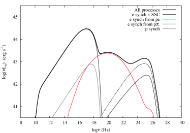
Figure 4: SED of the baseline Model A (thick solid line). The primary leptonic synchrotron and SSC components are plotted with thin solid line. Synchrotron emission from $p\pi$ pairs is shown with black dashed lines, while the $pe$ synchrotron spectrum is plotted with red solid line. Proton synchrotron radiation is overplotted with a grey line.

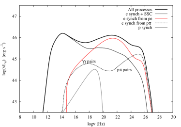
Figure 5: SED of the baseline Model B (thick solid line). The primary leptonic synchrotron and SSC components are plotted with thin solid line. The synchrotron spectrum of $pe$ pairs is plotted with red solid line, while synchrotron emission from secondary pairs produced through $p\pi$ interactions and photon-photon absorption of VHE $\gamma$-rays is shown with black dashed lines. Proton synchrotron radiation is overplotted with a grey line.

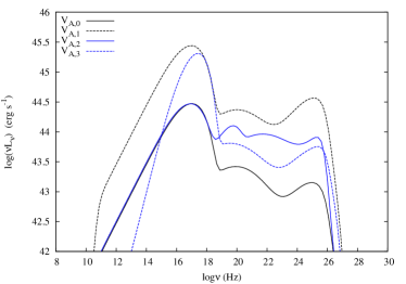
Figure 6: MW photon spectra obtained for the variants of the baseline Model A discussed in text.

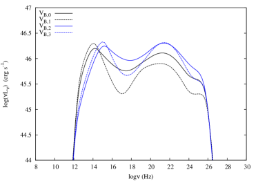
Figure 7: MW photon spectra obtained for the variants of the baseline Model B discussed in text.

The MW photon spectra obtained for the baseline Model A are shown in Fig. 4. The total emission when all processes are taken into account is plotted with a thick solid line. The derived synchrotron luminosity and peak frequency in this model are respectively $L_{\rm syn}\simeq 7\times 10^{44}$ erg/s and $\nu_{\rm s}\simeq 10^{17}$ Hz, which are more relevant to HBLs (e.g. Ghisellini & Tavecchio 2008). Application of the model to a particular HBL source, namely the prototype blazar Mrk 421, can be found in Mastichiadis et al. (2013) and Dimitrakoudis et al. (2014). The primary electron synchrotron and SSC emission are plotted with thin solid lines. The synchrotron emission of $pe$ and $p\pi$ pairs is shown with red solid and black dashed lines, respectively. Finally, the subdominant proton synchrotron component is plotted with a grey line. Although proton losses because of $pe$ pair production and photopion production are similar, the injection spectra of secondaries are different, thus resulting in very different emission signatures (see e.g. Figs. 7 and 4 in Kelner & Aharonian 2008 and DMPR12, respectively). Of particular interest is the broad synchrotron component of $pe$ pairs, which features photopair production as a physical process for the production of wide curved spectra outside the usual SSC framework.

We present the photon spectra for the baseline Model B in Fig. 5, where the different types of lines have the same meaning as in Fig. 4. The luminosity and peak frequency of the low-energy hump in this case are $L_{\rm syn}\simeq 3\times 10^{46}$ erg/s and $\nu_{\rm s}\simeq 10^{14}$ Hz, respectively, making Model B relevant to LBL emission. Similar to Model A, the contribution of the photopair synchrotron emission to the SED is dominant for a wide range of frequencies ($\sim 10^{18}-10^{24}$ Hz). Synchrotron emission from $p\pi$ pairs, on the other hand, has a harder spectrum than the emission from $pe$ pairs, and peaks at $\sim 10^{25}$ Hz. An additional feature of Model B is a component that peaks at $\sim 10^{16}$ Hz and is explained as synchrotron radiation of pairs produced through (internal) photon-photon absorption. In particular, the absorption of VHE $\gamma$-rays from $\pi^{0}$ decay initiates an EM cascade. This terminates whenever the synchrotron photons emitted by the pairs do not satisfy anymore the threshold condition for absorption on the photons of the low-energy component of the SED. For parameter values resulting in even higher optical depths for $\gamma$-ray absorption, the emission from the EM cascade dominates over the other components (see e.g. Mannheim & Biermann 1992; Petropoulou et al. 2013).

Summarizing, we showed that the emission from $pe$ pairs can fill, to an extend, the gap between the low-and high-energy humps of the SED (Fig. 4) or be the dominant photohadronic emission component in the hard X-ray/soft $\gamma$-ray regime (Fig. 5).

Model A variants

We investigate next three variants of the baseline Model A listed below:

• $V_{\rm A,0}$ for $\ell_{\rm e}^{\rm inj}=10^{-5.9},\gamma_{\rm p,\max}=1.2\times 10^{7}$ and $s_{\rm e}=2$

• $V_{\rm A,1}$ for $\ell_{\rm e}^{\rm inj}=10^{-4.9}$

• $V_{\rm A,2}$ for $\gamma_{\rm p,\max}=1.2\times 10^{8}$

• $V_{\rm A,3}$ for $s_{\rm e}=1$

with $V_{\rm A,0}$ corresponding to the baseline model. The respective photon spectra are presented in Fig. 6. The effect that a higher $\ell_{\rm e}^{\rm inj}$ has on the SED is straightforward, since it is translated to a higher photon number density in the source. When compared to the $V_{\rm A,0}$ case, the photohadronic components of the variant $V_{\rm A,1}$ have approximately $10$ times higher luminosity, i.e. they depend on $\ell_{\rm e}^{\rm inj}$ in a linear manner. This result should be compared to the one presented in DMPR12 (see Fig. 7 therein), where the photon target field for photohadronic interactions was the proton synchrotron radiation itself and the dependence on $\ell_{\rm p}^{\rm inj}$ was quadratic.

Example $V_{\rm A,2}$ demonstrates the effect of a higher $\gamma_{\rm p,\max}$, which now becomes $\sim 10\gamma_{\rm p,p\pi}^{\rm(th)}$, where $\gamma_{\rm p,p\pi}^{\rm(th)}\simeq 10^{7}$ for $\delta=30$ and $\nu_{\rm s}\simeq 10^{17}$ Hz (see eq. (7)). The $p\pi$ component peaks at approximately the same frequency as for the $V_{A,0}$ case, although the estimated shift according to eq. (42) is two orders of magnitude. The reason for this discrepancy is photon-photon absorption on the EBL, which attenuates the high energy part of the spectrum for the fiducial redhsift $z=0.14$. This is also indicated by an abrupt steepening of the high-energy part of the spectrum. Because the number density of protons depends only logarithmically on $\gamma_{\rm p,\max}$ for $s_{\rm p}=2$, the shift of the $pe$ and $p\pi$ components to higher luminosities is mainly caused by the fact that a larger number of protons satisfies the threshold conditions for photohadronic interactions with the primary electron synchrotron photons. The small bump that emerges at $\sim 10^{19}$ Hz is the peak of the proton synchrotron component. This is typically hidden by the other components but may appear for high $\gamma_{\rm p,\max}$ and hard ($s_{\rm p}\lesssim 2$) proton distributions. Finally, $V_{\rm A,2}$ is an indicative example of a theoretical spectrum that is approximately flat in $\nu F_{\nu}$ units and spans $\sim 6$ orders of magnitude in energy, with the $pe$ emission playing a key role.

The SED of $V_{\rm A,3}$ is obtained with a harder electron distribution that results in $\beta\simeq 0.1$ for frequencies above the synchrotron self-absorption one. We find that both photohadronic components of the SED have higher luminosity when compared to those of $V_{\rm A,0}$, with the harder synchrotron photon spectrum in this case being the reason. This can be understood by an inspection of eqs. (37) and (38), since changes in the proton loss rate are also reflected to the injection rate of secondaries. If $\beta_{1}=0.5$ and $\beta_{2}=0.1$, we find

$$\frac{f_{\rm p\pi}^{(2)}}{f_{\rm p\pi}^{(1)}}=\frac{(1-\beta_{2})}{\beta_{2}(\beta_{2}+2)}\frac{\beta_{1}(\beta_{1}+2)}{(1-\beta_{1})}\left(\frac{2\gamma_{\rm p}}{\gamma_{\rm p,p\pi}^{\rm(th)}}\right)^{\beta_{2}-\beta_{1}}\approx 8,$$ (44)

for $\gamma_{\rm p}=\gamma_{\rm p,p\pi}^{\rm(th)}$. This value agrees with the relative luminosity shift of the $p\pi$ component shown in Fig. 6, which is $\sim 0.7$ in logarithmic units. Similarly, the ratio of the $pe$ loss rates for two different spectral indices is

$$\frac{f_{pe}^{(2)}}{f_{pe}^{(1)}}=\frac{1-\beta_{2}}{1-\beta_{1}}\frac{I(\gamma_{\rm p},\beta_{2})}{I(\gamma_{\rm p},\beta_{1})}\left(\frac{2\gamma_{\rm p}}{\gamma_{\rm p,pe}^{\rm(th)}}\right)^{\beta_{2}-\beta_{1}}\approx 1.4\times 10^{-0.4c_{1}-0.25c_{2}},$$ (45)

where we used $\gamma_{\rm p}=\gamma_{\rm p,pe}^{\rm(th)}$ and approximated $\log I(\gamma_{\rm p},\beta)$ with a second order polynomial of $\beta$, for a fixed $\gamma_{\rm p}$; details can be found in the appendix. In the above, $c_{1}<0$, $c_{2}>0$ are the constants of the polynomial that depend on $\gamma_{\rm p}$, not strongly though. For $\gamma_{\rm p}\simeq 10^{5}$, the fitting of eq. (56) results in $c_{1}=-0.6$ and $c_{2}=0.01$. If we substitute these values into the equation above we find $f_{pe}^{(2)}/f_{pe}^{(1)}\approx 2.5$, which is in rough agreement with the increase found numerically (see Fig. 6).

Model B variants

The variants of Model B are summarized below:

• $V_{\rm B,0}$ for $\gamma_{\rm e,\min}=3\times 10^{2}$ and $s_{\rm e}=2.5$

• $V_{\rm B,1}$ for $\gamma_{\rm e,\min}=3\times 10^{2}$, $s_{\rm e}=3.0$

• $V_{\rm B,2}$ for $\gamma_{\rm e,\min}=10^{3}$, $s_{\rm e}=2.5$

• $V_{\rm B,3}$ for $\gamma_{\rm e,\min}=10^{3}$, $s_{\rm e}=3.0$

with $V_{\rm B,0}$ corresponding to the baseline model. By changing $\gamma_{\rm e,\min}$ and $s_{\rm e}$ we are able to test the way different peak frequencies and spectral indices of the synchrotron spectra affect the contribution of the $pe$ and $p\pi$ components to the SED. The respective photon spectra are shown in Fig. 7. First, let us compare variants with different $s_{\rm e}$ and fixed $\gamma_{\rm e,\min}$, i.e. $V_{\rm B,0}-V_{\rm B,1}$ and $V_{\rm B,2}-V_{\rm B,3}$. On the one hand, we find that softer synchrotron spectra result in a luminosity decrease of the $p\pi$ component, which is directly related to the decrease of $f_{\rm p\pi}$ (see right panel of Fig. 2). On the other hand, the luminosity of the $pe$ component either decreases (black lines) or remains approximately constant ( blue lines) as the synchrotron spectra become softer, which is related to the fact that the dependence of $f_{pe}$ on $\beta$ differs significantly between protons with different Lorentz factors– see also right panel of Fig. 2. Next we compare variants of the model with different $\gamma_{\rm e,\min}$ and fixed $s_{\rm e}$, i.e. $V_{\rm B,0}-V_{\rm B,2}$ and $V_{\rm B,1}-V_{\rm B,3}$. An increase of $\gamma_{\rm e,\min}$ by a factor of 3 shifts the peak frequency by $\sim$ one order of magnitude, and at the same time leads to an increase of both the $pe$ and $p\pi$ luminosities. The relative increase of the luminosity is larger for softer spectra, i.e. for $\beta=s_{\rm e}/2=1.5$. Equations (37) and (38) show that both energy loss rates depend on the peak frequency $\nu_{\rm s}$ as $f_{\rm i}\propto\nu_{\rm s}^{-1}\lambda(\beta,\epsilon_{\rm s})\left(\gamma_{\rm p,i}^{\rm(th)}\right)^{-\beta}$, where $\lambda(\beta,\epsilon_{\rm s})$ is defined in eq. (33). Since $\lambda$ is in good approximation independent of $\epsilon_{\rm s}$ for $\beta>1$ and $\gamma_{\rm p,i}^{\rm(th)}\propto\nu_{\rm s}^{-1}$ (see eqs. (7) and (8)) we find that $f_{\rm i}\propto\nu_{\rm s}^{\beta-1}$, which explains the larger luminosity increase of both components as $\beta$ becomes larger.

4.2.2 Neutrino emission

As already noted in §3.3, there is a direct link between the $\gamma$-ray and neutrino emission expected from a BL Lac object within our scenario. Figure 8 shows the combined photon and neutrino ($\nu_{\rm e}+\nu_{\mu}$) spectra obtained for the baseline Models A and B. The grey colored region marks the 0.1-100 PeV energy range and the bowties corresponding to the average BAT and LAT luminosities (Sambruna et al., 2010) are overplotted for comparison reasons. A few things that are worth commenting follow:

• the energy separation $R_{\nu,\gamma}$ of the neutrino and synchrotron from $p\pi$ pairs components is in agreement with eq. (41), at least for Model A. When applied to Model B, eq. (41) results in approximately three orders of magnitude larger separation in energy than the one depicted in Fig. 8. The reason is that eq. (41) has been derived under the assumption that there are protons energetic enough to satisfy the threshold condition for $p\pi$ interactions with photons having energy $\epsilon_{\rm s}$. In Model B, however, protons with $\gamma_{\rm p}=\gamma_{\rm p,\max}$ (see Table 1) do not satisfy this condition. By inverting eq. (7) and setting $\gamma_{\rm p,p\pi}^{\rm(th)}=\gamma_{\rm p,\max}$, we find that the threshold condition for photopion production is satisfied for $\nu\gtrsim 10^{17}$ Hz, which explains the derived value of $R_{\nu,\gamma}$.

• the neutrino peak energy lies in the $1-100$ PeV energy range in agreement with eq. (40). To estimate the peak neutrino energy for Model B, one has to replace $\nu_{\rm s}$ in eq. (40) with $\sim 10^{17}$ Hz, for the same reason explained above. Since $\delta\sim 10$, the peak energy of the neutrino spectrum is expected to be $\gtrsim 20$ PeV (see eq. (40)), unless the peak of the synchrotron component shifts to $\nu_{\rm s}\gtrsim 10^{17}$ Hz. In this regard, HBLs favour the production of neutrinos with a few PeV energy.

• in both models, which are described by very different parameters, the $pe$ , $p\pi$ and neutrino components of the blazar emission have comparable luminosity. Our scenario establishes a connection not only between the observed $\gamma$-ray flux and the expected neutrino flux from a BL Lac object, but also links the hard X-ray/soft $\gamma$-ray flux with both of them. We caution the reader that application of the model to specific sources, may lead to parameter values that suppress the $pe$ emission, and thus leading to $L_{\rm pe}\ll L_{\gamma}\sim L_{\nu}$ (see also discussion in §3.3). This is not, however, the generic case.

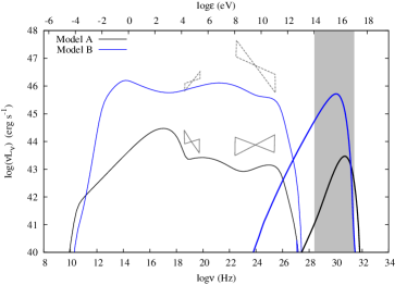
Figure 8: Combined photon (thin lines) and $\nu_{\rm e}+\nu_{\mu}$ (thick lines) spectra obtained for Models A (black lines) and B (blue lines). The grey colored region indicates the 0.1-100 PeV energy range. For comparison reasons, the average BAT and LAT luminosities for the first (solid lines) and third (dashed lines) BAT luminosity bins as defined in Sambruna et al. (2010) are also shown with bowties.

5 Discussion

In the present paper we examimed the impact of $pe$ pair production on the leptohadronic model of blazar emission. This process has played so far only a secondary role in modelling of MW spectra basically because the associated loss rate is typically smaller than the one of $p\pi$ interactions that act as a competing loss mechanism for protons. As a first order approximation, one could thus neglect the $pe$ process as a proton energy loss mechanism.

This has been indeed the standard approach in the literature so far, although it was noted (e.g. BSR90) that there are parameter regimes where the $pe$ loss rate becomes comparable or even surpasses the $p\pi$ loss rate. In our effort to reassess the role of the $pe$ process in the context of leptohadronic models of blazar emission, we compared the photohadronic loss rates for parameter values relevant to blazars (Figs. 2 and 3) using analytical expressions (eqs. (18), (21), (37) and (38)) that reveal the dependence of each loss rate on the various parameters. For the $pe$ loss rate, in particular, we derived a useful expression for the case of a power-law photon target field (eq. (38) and appendix), which faciliates quick comparisons for the losses of the two basic channels of photohadronic interactions.

Besides its role as an energy loss mechanism for high-energy protons, $pe$ pair production acts, more importantly, as an injection process of highly relativistic electron-positron pairs. These cool mainly through synchrotron radiation and, in principle, leave their radiative signature on the blazar MW spectrum. Yet, this aspect of $pe$ pair production has not attained a lot of attention. The $pe$ process has a distinct secondary production spectrum which is much broader than the one produced from photopion interactions (see e.g. Fig. 4 in DMPR12). In the simplest case, it is expected that the radiative signatures of secondaries produced through the aforementioned photohadronic processes will have non-overlapping spectra. Therefore, even in cases where $p\pi$ interactions dominate the losses, $pe$ secondary radiation could still be detectable, as its emission would not be hidden by the more luminous photopion component.

We showed that if the parameters of the source are such as to make the synchrotron emission of $p\pi$ pairs to appear in the GeV/TeV $\gamma$-ray regime, then the $pe$ component emerges in soft $\gamma$-rays (Figs. 4 and 5). This is a robust prediction of the leptohadronic model that can also serve as a an independent test for the existence of ultrarelativistic protons in blazar jets. We argued that the ‘smoking gun’ for proton acceleration in blazar jets is not only PeV neutrino emission but also the existence of a third photon component which lies between the UV/X-rays produced by primary electrons and the GeV/TeV $\gamma$ rays produced by $p\pi$ secondaries.

The numerical results presented in Section 4.2.1 were obtained for parameter sets that differed significantly, yet they indicated the appearance of a broad $\gamma$-ray hump with a peak in the sub-GeV regime (Figs. 6 and 7). This is an interesting issue, especially in the light of recent observations that reveal the presence of a wide high-energy component in LBL spectra that is not easily explained as SSC emission. Typical examples are the MW spectra of AP Librae (Fortin et al., 2010) and BL Lacartae (Abdo et al., 2011a), where in addition to the SSC emission, an external Compton (EC) component is required to explain the broad high-energy component, in a pure leptonic scenario. In principle, the MW variability predicted by the leptohadronic and SSC+EC scenarios will be different, and this can be used as a diagnostic tool for lifting possible model degeneracies. We plan to address this issue in a future publication.

As already noted in Mastichiadis et al. (2013), an important feature of the leptohadronic model under investigation is that it requires neither ultra-high energy protons ($\gamma_{\rm p,\max}\sim 10^{10}$) nor strong magnetic fields ($B\gtrsim 20$ G), in contrast to the more commonly adopted proton-synchrotron blazar model (e.g. Aharonian 2000; Mücke & Protheroe 2001). The first statement is a straightforward result of eq. (7), which also shows that the proton Lorentz factor at the $p\pi$ threshold and the observed peak frequency of the synchrotron spectrum are inversely proportional. This implies that as we move from HBLs to LBLs the required minimum proton energy for pion production on the synchrotron photons increases, and may even exceed the upper limit imposed by the Hillas condition, i.e. $\gamma_{\rm H}=eBr_{\rm b}/m_{\rm p}c^{2}$. We can use the requirement $\gamma_{\rm p,p\pi}^{\rm(th)}<\gamma_{\rm H}$ in order to set a lower limit on the magnetic field strength that is required by the model

$$B>9.5\times 10^{-2}\ {\rm G}\ \delta_{1}r_{\rm b,15}^{-1}\nu_{\rm s,16}^{-1}(1+z)^{-1},$$ (46)

where we made use of eq. (7). Thus, even for LBL sources with $\nu_{\rm s}\simeq 10^{14}$ Hz, our model does not require very strong magnetic fields, since the lower limit in this case would be $\sim 10$ G. The uncertainty introduced by the Doppler factor is small, since it lies typically in the range $10-50$ (e.g. Celotti et al. 1998; Maraschi et al. 1999), while a larger radius would simply relax this constraint. Concluding, strong magnetic fields ($\gtrsim 20$ G) are not necessary for the model to apply.

Since there is no a priori reason to exclude weak magnetic fields from our discussion, such as $B\sim 0.1$ G, SSC emission from primary electrons becomes relevant. For fixed $L_{\rm syn}$, $\nu_{\rm syn}$, $\delta$ and $r_{\rm b}$, weak magnetic fields favour SSC emission. Combining eqs. (6) and (10) we find that Compton scattering of photons at the peak of the low-energy component by electrons with $\gamma_{\rm e}$ take place in the Thomson regime, i.e. $\gamma_{\rm e}x_{\rm s}=0.08(\nu_{\rm s,16}/\nu_{\gamma,25})^{1/2}<3/4$. The typical frequency of the upscattered photons is then written as

$$\nu_{\rm ssc}\approx\gamma_{\rm e}^{2}\nu_{\rm s}\approx 10^{24}\ {\rm Hz}\ \delta_{1}^{2}(1+z)^{-1}\nu_{\gamma,25}^{-1}.$$ (47)

For low enough magnetic fields the observed $\gamma$-ray emission may be therefore the combined result of synchrotron emission from $p\pi$ secondary pairs and SSC emission of primary electrons (see Fig. 4). In this regard, the present leptohadronic scenario simplifies into a pure SSC model, by assuming only low enough values of the proton injection luminosity.

We constrained our analysis to cases where the emission from EM cascades is subdominant, as shown in Fig. 5. EM cascades are initiated by the absorption of VHE $\gamma$-rays that are produced by neutral pion decay. The optical depth for their absorption can be estimated as

$$\tau_{\gamma\gamma}\left(\epsilon_{\pi^{0}\rightarrow\gamma\gamma}^{\rm(th)}\right)\approx 9\times 10^{-4}\frac{L_{\rm syn,45}}{r_{\rm b,15}\delta_{1}^{3}\nu_{\rm s,16}(1+z)},$$ (48)

where the superscript “th” is used as a reminder of the parent proton’s energy (see eq. (7)). For the derivation of the above, we approximated (i) the cross-section for photon-photon absorption as $\sigma_{\gamma\gamma}=0.625\sigma_{\rm T}H(x_{\gamma}x-2)/(x_{\gamma}x)$, where $x$ and $x_{\gamma}$ denote the energies of two arbitrary photons in the comoving frame in units of $m_{\rm e}c^{2}$, and (ii) the low-energy component of the SED by the monoenergetic photon distribution defined in eq. (16). Only a fraction $\tau_{\gamma\gamma}$ of the VHE luminosity $L_{\pi^{0}\rightarrow\gamma\gamma}\simeq(1/2)f_{\rm p\pi}L_{\rm p}$ will appear in lower energies, with the ratio of the reprocessed to the total neutrino luminosity being approximately given by $\tau_{\gamma\gamma}L_{\pi^{0}\rightarrow\gamma\gamma}/L_{\nu}\approx(4/3)\tau_{\gamma\gamma}$, for $\tau_{\gamma\gamma}<1$. It is noteworthy that the absorption of VHE $\gamma$-rays from $\pi^{0}$ decay as well as the decay of charged pions results in the production of pairs with approximately the same energy (see also Petropoulou & Mastichiadis 2012). Thus, the absorbed VHE luminosity will reappear in the same $\gamma$-ray energy regime where the $p\pi$ component lies.

6 Summary

We explored some of the consequences that arise from the presence of relativistic protons in blazar jets. We focused on an often overlooked photohadronic process of astrophysical interest, namely the $pe$ pair production, and investigated its emission signatures on the SED of blazars. Motivated by the recent progress in high-energy neutrino astronomy (Aartsen et al., 2014), we adopted a theorical framework for the MW blazar emission, which associates the $\gamma$-ray flux with a high-energy (above a few PeV) neutrino signal. In this context, the low-energy hump of the SED is explained by synchrotron radiation of primary relativistic electrons, whereas the $\gamma$-ray emission is the result of photopion processes. After the electron and proton distributions that are necessary for explaining the double humped blazar SED have been determined, then the $pe$ component can be automatically defined, i.e. no additional free parameters are required.

We showed that for a wide range of parameters the synchrotron emission from $pe$ pairs fills the gap between the low and high energy components of the SED, i.e. between hard X-rays ($\gtrsim 40$ keV) and soft $\gamma$-rays ($\lesssim 40$ MeV). Although its peak luminosity is not always comparable to the one emitted in hard $\gamma$-rays, its radiative signature on the blazar spectrum may still be observable, as it is not hidden from other components. We demonstrated that the “$pe$ bump” of the SED is a robust prediction of the leptohadronic model, and as such, may provide indirect evidence for high-energy neutrino emission from BL Lac objects with a three-hump SED. Information is, therefore, required, either from current missions targeting in hard X-rays and soft $\gamma$-rays, e.g. NuSTAR (Harrison et al., 2013) and INTEGRAL (Lebrun et al., 2003; Ubertini et al., 2003), or from future satellites designed for soft $\gamma$-ray observations with high sensitivity, such as PANGU (Wu et al., 2014).

Appendix A Approximate Bethe-Heitler loss rate for a power-law photon distribution

The proton energy loss rate because of Bethe-Heitler pair production on an arbitrary isotropic photon field has been presented in B70 (see eq. (14)), while CZS92 have approximated function $\phi(\kappa)$ at different $\kappa$-regimes – see e.g. eqs. (3.13), (3.14) and (3.18), therein. Despite the good accuracy of the approximate solution, it is not so useful for the analytical manipulation of the integral in eq. (14), especially when the integration is to be performed for a power-law photon distribution ($n(\kappa)\propto\kappa^{-s}$).

Here we present a different approximation that facilitates the analytical calculation of $t_{pe}^{-1}$ for the case of a power-law photon distribution. Instead of focusing on $\phi(\kappa)$, we approximate the function $f(\kappa)=\phi(\kappa)/\kappa^{2}$. This has a peak of $\simeq 1$ at $\kappa\approx 47$ (see Fig. 2 in CZS92). When expressed in terms of $y=\ln\kappa$, function $f$ can be modeled as a bi-Gaussian function with four free parameters: the position of the peak $y_{0}$, the standard deviations $\sigma_{1}$ and $\sigma_{2}$ of the half Gaussians to the left and to the right of the peak, respectively, and the overall normalization $A$:

$$f(y)=f_{0}\left\{\begin{array}[]{cc}e^{-a_{1}\left(y-y_{0}\right)^{2}},&y\leq y_{0}\\ e^{-a_{2}\left(y-y_{0}\right)^{2}},&y>y_{0},\end{array}\right.$$ (51)

where $f_{0}=A/\sqrt{2\pi}$ and $a_{i}=1/2\sigma_{i}^{2}$. For $f_{0}=1.15$, $y_{0}=\ln 40$, $a_{1}=0.35$, and $a_{2}=0.09$, we find a good agreement with the exact expression in the range $7\lesssim\kappa\lesssim 5\times 10^{3}$ (see Fig. 9). For these values, the fractional error lies in the range $-5.8\%\leq\Delta f/f\leq 3.4\%$ and has a mean value of $\sim 0.1\%$.

Figure 9: Comparison of the exact (solid line) and bi-Gaussian approximation (dashed line) of the function $f=\phi(\kappa)/\kappa^{2}$.

Using the bi-Gaussian approximation for the calculation of the integral in eq. (14), for the photon distribution of eq. (27), we find

$$I_{0}=N_{0}\int_{y_{\min}}^{y_{\max}}dye^{-\beta y}f(y)=N_{0}I(\gamma_{\rm p},\beta),$$ (52)

where $N_{0}=m_{\rm e}c^{2}n^{\prime}_{0}(2\gamma_{\rm p}x_{\rm s})^{\beta+1}$, $y_{\min}=\max[\ln 2,\ln(2\gamma_{\rm p}x_{\min})]$ and $y_{\max}=\ln(2\gamma_{\rm p}x_{\max})$. The integral can be now performed analytically and results in

$$\frac{I(\gamma_{\rm p},\beta)}{f_{0}e^{-\beta y_{0}}}=\left\{\begin{array}[]{ll}\!f_{1}erf(x_{1})\biggr{\rvert}_{y_{\min}}^{y_{0}}\!\!+\!f_{2}erf(x_{2})\biggr{\rvert}_{y_{0}}^{y_{\max}},&y_{\min}\leq y_{0}\leq y_{\max}\\ \!f_{1}erf(x_{1})\biggr{\rvert}_{y_{\min}}^{y_{\max}},&y_{\max}\leq y_{0}\\ \!f_{2}erf(x_{2})\biggr{\rvert}_{y_{\min}}^{y_{\max}},&y_{\min}\geq y_{0},\end{array}\right.$$ (56)

where $erf(x)$ is the error function and

$$f_{i} = \sqrt{\frac{\pi}{4a_{i}}}e^{\beta^{2}/4a_{i}}$$ (57)

$$x_{i} = \frac{\beta+2a_{i}(y-y_{0})}{2\sqrt{a_{i}}}$$ (58)

for $i=1,2$. For a fixed proton energy, the logarithm of $I(\gamma_{\rm p},\beta)$ can be modelled by a second order polynomial of the spectral index, i.e. $\log I(\gamma_{\rm p},\beta)=c_{0}+c_{1}\beta+c_{2}\beta^{2}$, with the numerical values of the constants $c_{i}$ depending on $\gamma_{\rm p}$. Figure 10 shows $I(\gamma_{\rm p},\beta)$ in logarithmic units, as a function of $\beta$ (points) for $\gamma_{\rm p}=10^{7}$. The red line is the result of a non-linear fit with $c_{0}=0.62$, $c_{1}=-1.7$ and $c_{2}=0.29$. We verified that this result is not sensitive on the the ratio of the minimum and maximum energies of the photon distribution. The dependence of $I(\gamma_{\rm p},\beta)$ on $\xi=2\gamma_{\rm p}/\gamma_{\rm p,BH}^{\rm(th)}$, where $\gamma_{\rm p,BH}^{\rm(th)}=4\times 10^{4}$, is exemplified in Fig. 11 for two values of the spectral index $\beta$. Interestingly, $I(\gamma_{\rm p},\beta)$ is constant for a wide range of $\xi$ values, and starts to decrease with $\xi$ only for large enough values (see Fig. 11).

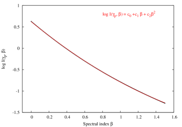
Figure 10: Plot of $\log I(\gamma_{\rm p},\beta)$ as a function of the spectral index for $\gamma_{\rm p}=10^{7}$ (points). The red line is the result of a second order polynomial fit with constants $c_{0}=0.62$, $c_{1}=-1.7$ and $c_{2}=0.29$. Other parameters used are $x_{\max}=2.7\times 10^{-5}$ and $x_{\min}=10^{-4}x_{\max}$.

Figure 11: Log-log plot of $I(\gamma_{\rm p},\beta)$ as a function of $\xi=2\gamma_{\rm p}/\gamma_{\rm p,BH}^{\rm(th)}$ for $\beta=0.1$ (solid line) and $\beta=1$ (dashed line). Other parameters used are $x_{\max}=2.7\times 10^{-5}$, $x_{\min}=10^{-4}x_{\max}$, and $\gamma_{\rm p,BH}^{\rm(th)}=4\times 10^{4}$.

The dimensionless loss rates $f_{pe}$ calculated using the CZS92 and bi-Guassian approximations for the case of a power-law photon distribution are presented in Fig. 12. The parameters used are: $L_{\rm syn}=10^{45}$ erg/s, $r_{\rm b}=3\times 10^{15}$ cm, $\delta=30$, $\nu_{\rm s}=10^{16}$ Hz, $x_{\rm s}=x_{\max}=2.7\times 10^{-6}$ and $x_{\min}=10^{-4}x_{\max}$. We show the results for two spectral indices, i.e. $\beta=1$ (red) and $0.1$ (black). The normalization of the photon distribution for $\beta=1$ and $\beta=0.1$ is $n^{\prime}_{0}=10^{13.3}(m_{\rm e}c^{2})^{-1}$ and $10^{14.2}(m_{\rm e}c^{2})^{-1}$ cm^-3 erg^-1, respectively. Except for the difference close to the threshold, where the fractional error of the approximation takes its maximum value (see Fig. 9), the two results are in very good agreement. We verified this for different different values of the ratio $x_{\max}/x_{\min}$ and spectral indices.

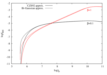
Figure 12: Comparison of $f_{pe}$ when calculated using the CZS92 (solid line) and bi-Gaussian (dashed line) approximations for a power-law photon distribution with $\beta=0.1$ (black lines) and $\beta=1$ (red lines). For the parameters used, see text.

References

- Aartsen et al. (2014) Aartsen M. G. et al., 2014, Physical Review Letters, 113, 101101
- Abdo et al. (2011a) Abdo A. A. et al., 2011a, Astrophysical Journal, 730, 101
- Abdo et al. (2011b) Abdo A. A. et al., 2011b, Astrophysical Journal, 736, 131
- Aharonian et al. (2007) Aharonian F. et al., 2007, Astrophysical Journal Letters, 664, L71
- Aharonian (2000) Aharonian F. A., 2000, New Astron., 5, 377
- Aleksić et al. (2011) Aleksić J. et al., 2011, Astrophysical Journal Letters, 730, L8
- Atoyan & Dermer (2001) Atoyan A., Dermer C. D., 2001, Physical Review Letters, 87, 221102
- Atoyan & Dermer (2003) Atoyan A. M., Dermer C. D., 2003, Astrophysical Journal, 586, 79
- Beall & Bednarek (1999) Beall J. H., Bednarek W., 1999, Astrophysical Journal, 510, 188
- Bednarek & Protheroe (1999) Bednarek W., Protheroe R. J., 1999, Monthly Notices of the Royal Astronomical Society, 302, 373
- Begelman et al. (1990) Begelman M. C., Rudak B., Sikora M., 1990, Astrophysical Journal, 362, 38
- Beringer et al. (2012) Beringer J. et al., 2012, Phys. Rev. D, 86, 010001
- Biermann & Strittmatter (1987) Biermann P. L., Strittmatter P. A., 1987, Astrophysical Journal, 322, 643
- Bloom & Marscher (1996) Bloom S. D., Marscher A. P., 1996, Astrophysical Journal, 461, 657
- Blumenthal (1970) Blumenthal G. R., 1970, Physical Review D, 1, 1596
- Böttcher (2010) Böttcher M., 2010, ArXiv e-prints
- Böttcher & Dermer (1998) Böttcher M., Dermer C. D., 1998, Astrophysical Journal Letters, 501, L51
- Böttcher et al. (2013) Böttcher M., Reimer A., Sweeney K., Prakash A., 2013, Astrophysical Journal, 768, 54
- Cao & Wang (2014) Cao G., Wang J., 2014, Astrophysical Journal, 783, 108
- Celotti et al. (1998) Celotti A., Fabian A. C., Rees M. J., 1998, Monthly Notices of the Royal Astronomical Society, 293, 239
- Cerruti et al. (2011) Cerruti M., Zech A., Boisson C., Inoue S., 2011, in SF2A-2011: Proceedings of the Annual meeting of the French Society of Astronomy and Astrophysics, Alecian G., Belkacem K., Samadi R., Valls-Gabaud D., eds., pp. 555–558
- Chodorowski et al. (1992) Chodorowski M. J., Zdziarski A. A., Sikora M., 1992, Astrophysical Journal, 400, 181
- Costamante et al. (2001) Costamante L. et al., 2001, Astronomy & Astrophysics, 371, 512
- Dermer & Schlickeiser (1993) Dermer C. D., Schlickeiser R., 1993, Astrophysical Journal, 416, 458
- Dermer et al. (1992) Dermer C. D., Schlickeiser R., Mastichiadis A., 1992, Astronomy & Astrophysics, 256, L27
- Dimitrakoudis et al. (2012) Dimitrakoudis S., Mastichiadis A., Protheroe R. J., Reimer A., 2012, Astronomy & Astrophysics, 546, A120
- Dimitrakoudis et al. (2014) Dimitrakoudis S., Petropoulou M., Mastichiadis A., 2014, Astroparticle Physics, 54, 61
- Fortin et al. (2010) Fortin P. et al., 2010, in 25th Texas Symposium on Relativistic Astrophysics
- Foschini et al. (2013) Foschini L., Bonnoli G., Ghisellini G., Tagliaferri G., Tavecchio F., Stamerra A., 2013, Astronomy & Astrophysics, 555, A138
- Fossati et al. (1998) Fossati G., Maraschi L., Celotti A., Comastri A., Ghisellini G., 1998, Monthly Notices of the Royal Astronomical Society, 299, 433
- Franceschini et al. (2008) Franceschini A., Rodighiero G., Vaccari M., 2008, Astronomy & Astrophysics, 487, 837
- Ghisellini (2001) Ghisellini G., 2001, in Astronomical Society of the Pacific Conference Series, Vol. 234, X-ray Astronomy 2000, Giacconi R., Serio S., Stella L., eds., p. 425
- Ghisellini & Madau (1996) Ghisellini G., Madau P., 1996, Monthly Notices of the Royal Astronomical Society, 280, 67
- Ghisellini & Tavecchio (2008) Ghisellini G., Tavecchio F., 2008, Monthly Notices of the Royal Astronomical Society, 387, 1669
- Giovanoni & Kazanas (1990) Giovanoni P. M., Kazanas D., 1990, Nature, 345, 319
- Globus et al. (2014) Globus N., Allard D., Mochkovitch R., Parizot E., 2014, ArXiv e-prints
- Harrison et al. (2013) Harrison F. A. et al., 2013, Astrophysical Journal, 770, 103
- IceCube Collaboration (2013) IceCube Collaboration, 2013, Science, 342
- Kataoka et al. (2001) Kataoka J. et al., 2001, Astrophysical Journal, 560, 659
- Kelner & Aharonian (2008) Kelner S. R., Aharonian F. A., 2008, Physical Review D, 78, 034013
- Kirk & Mastichiadis (1989) Kirk J. G., Mastichiadis A., 1989, Astronomy & Astrophysics, 213, 75
- Konopelko et al. (2003) Konopelko A., Mastichiadis A., Kirk J., de Jager O. C., Stecker F. W., 2003, Astrophysical Journal, 597, 851
- Lebrun et al. (2003) Lebrun F. et al., 2003, Astronomy & Astrophysics, 411, L141
- Mannheim (1993) Mannheim K., 1993, Astronomy & Astrophysics, 269, 67
- Mannheim & Biermann (1992) Mannheim K., Biermann P. L., 1992, Astronomy & Astrophysics, 253, L21
- Mannheim et al. (1991) Mannheim K., Biermann P. L., Kruells W. M., 1991, Astronomy & Astrophysics, 251, 723
- Maraschi et al. (1999) Maraschi L. et al., 1999, Astrophysical Journal Letters, 526, L81
- Maraschi et al. (1992) Maraschi L., Ghisellini G., Celotti A., 1992, Astrophysical Journal Letters, 397, L5
- Mastichiadis & Kirk (1995) Mastichiadis A., Kirk J. G., 1995, Astronomy & Astrophysics, 295, 613
- Mastichiadis & Kirk (1997) Mastichiadis A., Kirk J. G., 1997, Astronomy & Astrophysics, 320, 19
- Mastichiadis et al. (2013) Mastichiadis A., Petropoulou M., Dimitrakoudis S., 2013, Monthly Notices of the Royal Astronomical Society, 434, 2684
- Mastichiadis et al. (2005) Mastichiadis A., Protheroe R. J., Kirk J. G., 2005, A&A, 433, 765
- Mücke et al. (2000) Mücke A., Engel R., Rachen J. P., Protheroe R. J., Stanev T., 2000, Computer Physics Communications, 124, 290
- Mücke & Protheroe (2001) Mücke A., Protheroe R. J., 2001, Astroparticle Physics, 15, 121
- Mücke et al. (2003) Mücke A., Protheroe R. J., Engel R., Rachen J. P., Stanev T., 2003, Astroparticle Physics, 18, 593
- Murase et al. (2014) Murase K., Inoue Y., Dermer C. D., 2014, Physical Review D, 90, 023007
- Petropoulou (2014a) Petropoulou M., 2014a, Monthly Notices of the Royal Astronomical Society, 442, 3026
- Petropoulou (2014b) Petropoulou M., 2014b, ArXiv e-prints
- Petropoulou et al. (2013) Petropoulou M., Arfani D., Mastichiadis A., 2013, Astronomy & Astrophysics, 557, A48
- Petropoulou et al. (2014a) Petropoulou M., Giannios D., Dimitrakoudis S., 2014a, ArXiv e-prints
- Petropoulou et al. (2014b) Petropoulou M., Lefa E., Dimitrakoudis S., Mastichiadis A., 2014b, Astronomy & Astrophysics, 562, A12
- Petropoulou & Mastichiadis (2012) Petropoulou M., Mastichiadis A., 2012, Monthly Notices of the Royal Astronomical Society, 421, 2325
- Protheroe & Johnson (1996) Protheroe R. J., Johnson P. A., 1996, Astroparticle Physics, 4, 253
- Raiteri et al. (2012) Raiteri C. M. et al., 2012, Astronomy & Astrophysics, 545, A48
- Sahu et al. (2013) Sahu S., Oliveros A. F. O., Sanabria J. C., 2013, Physical Review D, 87, 103015
- Sambruna et al. (2010) Sambruna R. M. et al., 2010, Astrophysical Journal, 710, 24
- Schmitt (1968) Schmitt J. L., 1968, Nature, 218, 663
- Schuster et al. (2002) Schuster C., Pohl M., Schlickeiser R., 2002, Astronomy & Astrophysics, 382, 829
- Sikora et al. (1994) Sikora M., Begelman M. C., Rees M. J., 1994, Astrophysical Journal, 421, 153
- Sikora et al. (1987) Sikora M., Kirk J. G., Begelman M. C., Schneider P., 1987, Astrophysical Journal Letters, 320, L81
- Sironi et al. (2013) Sironi L., Spitkovsky A., Arons J., 2013, Astrophysical Journal, 771, 54
- Sobolewska et al. (2014) Sobolewska M. A., Siemiginowska A., Kelly B. C., Nalewajko K., 2014, Astrophysical Journal, 786, 143
- Stanev et al. (2000) Stanev T., Engel R., Mücke A., Protheroe R. J., Rachen J. P., 2000, Physical Review D, 62, 093005
- Stecker (1968) Stecker F. W., 1968, Physical Review Letters, 21, 1016
- Stecker et al. (1991) Stecker F. W., Done C., Salamon M. H., Sommers P., 1991, Physical Review Letters, 66, 2697
- Ubertini et al. (2003) Ubertini P. et al., 2003, Astronomy & Astrophysics, 411, L131
- Ulrich et al. (1997) Ulrich M.-H., Maraschi L., Urry C. M., 1997, Ann. Rev. Astron. Asrophys., 35, 445
- Waxman & Bahcall (1997) Waxman E., Bahcall J., 1997, Physical Review Letters, 78, 2292
- Weidinger & Spanier (2013) Weidinger M., Spanier F., 2013, in European Physical Journal Web of Conferences, Vol. 61, European Physical Journal Web of Conferences, p. 5009
- Wu et al. (2014) Wu X., Su M., Bravar A., Chang J., Fan Y., Pohl M., Walter R., 2014, ArXiv e-prints