A Scaling Relation for Dangerously Irrelevant Symmetry-Breaking Fields

Abstract

We propose a scaling relation for critical phenomena in which a symmetry-breaking field is dengerously irrelevant. We confirm its validity on the 6-state clock model in three and four dimensions by numerical simulation. In doing so, we point out the problem in the previously-used order parameter, and present an alternative evidence based on the mass-dependent fluctuation.

Irrelevant scaling fields are ubiquitous. While they play minor roles in most cases, some of them are quite relevant in the usual sense of the word. A text-book example is the $\phi^{4}$ term in the $\phi^{4}$ theory above the upper critical dimension Cardy (1996). In the present Letter, we discuss cases where such a dangerously-irrelevant scaling field reduces the symmetry of the system, and demonstrate that it yields a new scaling relation.

Consider a renormalization-group flow diagram including two fixed points; one describing the critical point and the other the ordered phase. In principle it is possible that some irrelevant perturbative field at the critical fixed point contains some scaling field that is relevant at the one of the two. In particular, when the perturbation is symmetry-reducing, it can happen that both fixed points lie on the same manifold characterized by zero of the perturbative field as illustrated in Fig. 1. In such cases, even if the perturbation almost dies out at some length scale, say $\xi$, it may recover its amplitude at larger length scale, say $\xi^{\prime}$. When the system size is between the two scaling lengths, $\xi\ll L\ll\xi^{\prime}$, the system may look ordered but still no effect of the symmetry breaking is visible. It may then appear that an intermediate phase exists where the system acquires an emergent symmetry. A classical example of this type of renormalization group flow is the $q$-state clock model in three dimensions Oshikawa (2000), and its continuous-spin counterpart.

In fact, such an intermediate phase really exists in two dimensions José et al. (1977). However, based on the Monte Carlo simulation results, Miyashita Miyashita (1997) suggested a simpler scenario for the three dimensional case. Furthermore, Oshikawa Oshikawa (2000) pointed out that the existence of the intermediate phase is very unlikely because the low-temperature phase is already ordered in the pure model in three dimensions, and that the whole low-temperature phase is controlled by the zero-temperature fixed point, in contrast to the two-dimensional case. The two-dimensional quantum SU($N$) Heisenberg model may offer a quantum-mechanical example. While the ground state of this model is the Neèl state upto $N=4$, the valence bond solid state takes over for $N\geq 5$ Kawashima and Tanabe (2007). When described in terms of effective spins representing the direction of the ordered valence bond pattern, the system can be regarded as a model analogous to the clock model. It was discovered that the order parameter distribution function is almost circular symmetric, indicating the extremely small effect of the anisotropy. Later, an additional term was introduced Sandvik (2007); Harada et al. (2007, 2013) to control the quantum fluctuation and drive the system to the true transition point.

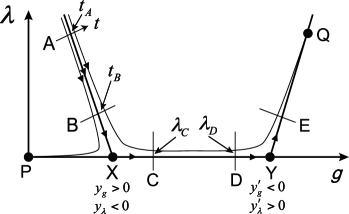
Figure 1: The generic renormarization flow diagram with four fixed points: P, Q, X, and Y.

It is now widely accepted that in three dimensions there is no partially ordered phase with the emergent symmetry. However, disagreement still persists concerning the scaling relation that relates the scaling exponent $\nu^{\prime}$ that characterizes the longer correlation length and $\nu$ characterizing the shorter correlation length. In this Letter, we propose a new general scaling relation and verify its validity by Monte Carlo simulation of the $XY$ model with the $Z_{q}$ scaling field. To verify the validity of the new scaling relation, below we first present the numerical results of the anisotropy order parameter, often referred to as $\phi_{6}$, suggesting that previously-proposed scaling relations do not actually hold. We further argue that, unlike the conventional finite-size scaling, the scaling plot of $\phi_{6}$ is not fully supported by renormalization group picture; we present a more complete scaling argument supported by Monte Carlo simulation.

Previously, a scaling relation was proposed by Ueno et al. Ueno and Mitsubo (1991) and by Oshikawa Oshikawa (2000). Their argument is based on the basic assumption that there is a well defined domain wall splitting the whole system and the excess free-energy caused by the domain walls is the scaling variable. The excess free-energy density per area of the domain wall may be given by the symmetry-breaking field renormalized upto the scale of locally-correlated volume, $\lambda(\xi)\sim\lambda\xi^{y_{\lambda}}$ ($y_{\lambda}$ represents the scaling exponent of the symmetry-breaking field at the critical fixed point). The total domain-wall free-energy, then, may be $L^{d-1}\lambda(\xi)\sim(L/\xi^{-y_{\lambda}/(d-1)})^{d-1}$. This yields

$$\frac{\nu^{\prime}}{\nu}=\frac{-y_{\lambda}}{d-1}.$$ (1)

Lou, Sandvik, and Balents Lou et al. (2007) presented a similar argument, but they argued that the effect of the anisotropy free-energy comes from the volume instead of the domain-walls. Therefore, they multiply the renormalized field by the number of correlated volumes, to obtain $(L/\xi)^{d}\lambda\xi^{y_{\lambda}}$ $=\lambda(L/\xi^{1-y_{\lambda}/d})^{d}$. This means

$$\frac{\nu^{\prime}}{\nu}=1+\frac{-y_{\lambda}}{d}.$$ (2)

Here we present another scaling relation that is more general and differs from the previous ones. We again consider the generic renormalization group flow of Fig. 1. The bare Hamiltonian is along the short line near the point “A” parametetrized by $t$ so that $t=0$ corresponds to the critical point. If we start from the point $t=0$ on this line, the scaling flow takes us to the critical fixed point “X”, where $g=g_{\rm X}$ and $\lambda=0$. If we start from a point with $t=t_{\rm A}>0$ and $\lambda=\lambda_{\rm A}>0$, the scaling flow goes through the points “C” $(|g_{\rm C}-g_{\rm X}|=O(1)$, $\lambda_{\rm C}\ll 1)$, “D” $(|g_{\rm D}-g_{\rm Y}|=O(1)$, $\lambda_{\rm D}\ll 1)$, and approaches the second fixed point “Y” around which renormalization group flow is characterized by scaling exponents $y^{\prime}_{g}<0$ for the variable $g$ and $y^{\prime}_{\lambda}>0$ for the variable $\lambda$. Because of the presence of $\lambda$, the flow deviates from “Y”, goes through the point “E” $(\lambda_{\rm E}=O(1))$ and eventually reaches some other fixed point. The shorter correlation length $\xi$ equals $\Lambda_{\rm AC}$, i.e., the length scale that has to be renormalized to go from “A” to “C”, whereas the longer correlation length $\xi^{\prime}$ equals $\Lambda_{\rm AE}$. The critical intervals are $BC$ and $DE$. For the interval $BC$, we have $\lambda_{\rm C}\sim\xi^{y_{\lambda}}.$ For $DE$, $1\sim\lambda_{\rm E}\sim\lambda_{\rm D}(\Lambda_{\rm DE})^{y^{\prime}_{\lambda}},$ which yields $\Lambda_{\rm DE}\sim(\lambda_{\rm D})^{-1/y^{\prime}_{\lambda}}$ $\propto(\lambda_{\rm C})^{-1/y^{\prime}_{\lambda}}$ $\sim\xi^{-y_{\lambda}/y^{\prime}_{\lambda}}.$ Therefore,

$$\xi^{\prime}\propto\Lambda_{\rm BC}\Lambda_{\rm DE}\sim\xi^{1+\frac{-y_{\lambda}}{y^{\prime}_{\lambda}}}.$$

Thus we have arrived at

$$\frac{\nu^{\prime}}{\nu}=1+\frac{-y_{\lambda}}{y^{\prime}_{\lambda}}.$$ (3)

In order to determine which scaling relation should apply, we need independent estimates of the scaling indices, $\nu$, $\nu^{\prime}$, $y_{\lambda}$, and $y^{\prime}_{\lambda}$, in (3). Here we consider the $XY$ model in three dimensions with the $Z_{q}$ anisotropy field.

$$H=-J\sum_{({\mbox{\boldmath$r$}},{\mbox{\boldmath$r$}}^{\prime})}\cos(\theta({\mbox{\boldmath$r$}})-\theta({\mbox{\boldmath$r$}}^{\prime}))-\lambda_{q}\sum_{{\mbox{\boldmath$r$}}}\cos(q\theta({\mbox{\boldmath$r$}}))$$

As for $\nu$, previous estimates of the pure $XY$ universality class is available, $\nu=0.6717(1)$ Campostrini et al. (2006). As for $y_{\lambda}$, previous calculation according to the first-order $\varepsilon$-expansion Oshikawa (2000) leads,

$$y_{\lambda}=4-q+\varepsilon\left(\frac{q}{2}-1-\frac{q(q-1)}{10}\right),$$

e.g., $y_{\lambda}=-0.2$ for $q=4$ and $=-3.0$ for $q=6$. In addition to this $\varepsilon$-expansion, Monte Carlo estimates of the $y_{\lambda}$ upto $q=4$ are available Hasenbusch and Vicari (2011). In Fig. 2, we plot the estimated scaling eigenvalues and their extrapolation by the second-order polynomial along with the result of the first-order $\varepsilon$-expansion. The Monte Carlo estimation of $y_{\lambda}$s reveals a surprisingly good agreement with the first-order $\varepsilon$-expansion, while the second-order polynomial fitting is slightly deviate from the $\varepsilon$-expansion at $q=6$. From this figure, we estimate $y_{\lambda}=-2.5(2)$ for $q=6$.

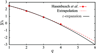
Figure 2: (color online) The estimated scaling eigenvalues from Ref. Hasenbusch and Vicari (2011)(symbols), the second-order polynomial fitting to them (dashed curve), and the result of the first-order $\varepsilon$-expansion (solid curve).

As for $y^{\prime}_{\lambda}$, an argument Oshikawa (2000) suggests that the quadratic fluctuation around the ordered configuration is essential at the NG fixed point, leading to $y^{\prime}_{\lambda}=2$, analogous to the scaling eigenvalue of the $\phi^{2}$ field in the Gaussian field theory. Finally, we consider $\nu^{\prime}$. In order to estimate $\nu^{\prime}$ we need a proper scaling variable which obeys a finite size scaling with $\nu^{\prime}$.

In the previous studies, an order parameter that characterizes the symmetry reduction from $U(1)$ to $Z_{6}$,

$$\phi_{6}\equiv\langle\cos(6\theta_{0})\rangle$$

was analyzed by assuming $\phi_{6}\sim f(tL^{1/\nu^{\prime}})$ Oshikawa (2000); Lou et al. (2007). Here, $\theta_{0}$ is the angle of the average magnetization, i.e.,

$$(m_{0}\cos\theta_{0},m_{0}\sin\theta_{0})\equiv\frac{1}{N}\sum_{{\mbox{\boldmath$r$}}}(\cos\theta({\mbox{\boldmath$r$}}),\sin\theta({\mbox{\boldmath$r$}})),$$

and $\langle\cdots\rangle$ represents a thermal average. In Fig. 3(a), we show the finite size scaling of $\phi_{6}$ against $(T_{c}-T)L^{1/\nu^{\prime}}$ with $\nu^{\prime}=1.45$ which is estimated from Bayesian method Harada (2011). Estimated $\nu^{\prime}$ considerably deviated from Ueno’s scaling relation (1) and Lou’s scaling relation (2); they give $\nu^{\prime}\simeq 0.84$ and $\nu^{\prime}\simeq 1.23$ from known exponents $\nu$ and $y_{\lambda}$, respectively. Indeed, when we use even relatively acceptable Lou’s value, $\nu^{\prime}=1.23$, the overlap of the data become clearly worse (see Fig. 3(b)). Therefore scaling relations (1) and (2) seem to fail in the present critical phenomenon.

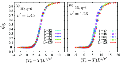
Figure 3: (color online) The finite size scaling of $\phi_{6}$ for the $Z_{6}$-anisotropic $XY$ model with $\lambda_{6}/J=5$ in three dimensions. (a) $\nu^{\prime}=1.45$, (b) $\nu^{\prime}=1.23$. For the scaling we used the date set of $(T_{c}-T)/J\leq 0.4$.

Note, however, this finite-size scaling plot of $\phi_{6}$ is different from conventional finite-size scaling in that it is not clear whether we would obtain a perfect data collapse even in the limit of infinite system size. More specifically, to regard $\phi_{6}$ as a scaling operator in its full value range, $\theta_{0}$ must be dimensionless scaling operator. However, at the NG fixed point, it has a non-zero scaling dimension Oshikawa (2000). Therefore, the meaning of scaling analysis based on $\phi_{6}$ is not clear, even if the resulting plottings may look reasonably good . We propose another scaling variable whose scaling form is directly calculated from the effective theory around the NG fixed point.

Suppose that we start from the high-temperature phase and gradually cool the system passing the transition point. Because of the asymptotic U(1) symmetry, the ordering angle $\theta_{0}$, selected by the spontaneous symmetry-breaking, can be any value in the interval $[0,2\pi)$. Once the ordering angle has been selected, it does not change (in a finite time) and determines the “mass of the particles”. More specifically, the effective Hamiltonian that characterizes the system at the length scale larger than the (first) correlation length $\xi$ can be obtained by expanding $\mathcal{H}=\int d^{d}\bm{r}^{\prime}\left[\frac{1}{2}(\bm{\nabla}\theta)^{2}-\lambda_{q}^{\prime}\cos q\theta\right]$ in terms of the small fluctuation around the direction of the spontaneous ordering, $\phi\equiv\theta-\theta_{0}$:

$$\mathcal{H}_{\theta_{0}}=\frac{1}{2}\int d^{d}\bm{r}^{\prime}\left[(\bm{\nabla}\phi)^{2}+\lambda_{q}^{\prime}q^{2}\cos(q\theta_{0})\phi^{2}\right]\\ -\lambda_{q}^{\prime}L^{\prime d}\cos q\theta_{0}+O(\phi^{3}).$$ (4)

Note that $\bm{r}^{\prime}$ implies the renormalized length $\bm{r}^{\prime}\sim\bm{r}/\xi$. This Gaussian field theory indicates that Fourier modes of fluctuation are governed by renormalized anisotropy and macroscopic orientation $\theta_{0}$ as

$$\langle|\phi_{\bm{k}^{\prime}}|^{2}\rangle_{\theta_{0}}\sim\frac{1}{k^{\prime 2}+\lambda^{\prime}_{q}q^{2}\cos q\theta_{0}},$$ (5)

where $\langle\cdots\rangle_{\theta_{0}}$ means the average with the condition that the macroscopic orientation is equal to $\theta_{0}$. Note that every quantity in this expression is normalized upto the length scale $\xi$, i.e., $\lambda^{\prime}_{q}=\lambda_{q}\xi^{y_{\lambda}}$, ${\mbox{\boldmath$r$}}^{\prime}\equiv{\mbox{\boldmath$r$}}/\xi$, and $k^{\prime}\equiv k\xi$. Then, if we take the wavenumber $k^{\prime}$ as $2\pi/(L/\xi)$, $\langle|\phi_{\bm{k}^{\prime}}|^{2}\rangle_{\theta_{0}}$ obeys the scaling form $\langle|\phi_{\bm{k}^{\prime}}|^{2}\rangle_{\theta_{0}}\sim(L/\xi)^{2}f(L/\xi^{a})$ with $a\equiv 1-y_{\lambda}/2$. This form indicates that $\xi^{\prime}\sim\xi^{a}$ or $\nu^{\prime}/\nu=a$.

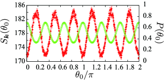
Figure 4: (color online) The angle dependent spin structure factor $S_{\bm{k}}(\theta_{0})$ (filled circle) and the probability distribution of ordering angle $\theta_{0}$ (open circle) for the $Z_{6}$-anisotropic $XY$ model with $\lambda_{6}/J=5$, $L=64$ at $T/J=2.0<T_{c}/J$ ($T_{c}/J=2.202$) in three dimensions.

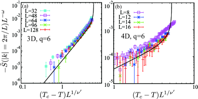
Figure 5: (color online) Log-log plot of the angular Fourier transform of the angle dependent spin-structure factor $\tilde{S}$ for the $Z_{6}$-anisotropic $XY$ model with $\lambda_{6}/J=5$ in three dimensions (a) and in four dimensions(b). (a) the finite-size scaling plot assuming $\omega=1.983$ and $\nu^{\prime}=1.511$ . (b) the finite-size scaling plot assuming $\omega=2.0$ and $\nu^{\prime}=1$ in four dimension. The critical temperatures $T_{c}/J=2.202$ for three dimension and $T_{c}/J=3.3143$ for four dimenstions are estimated from the binder ratios of the magnetization. The solid curves are the fittings of the scaling function (9) assuming $\nu=0.6717$, $x_{h}=0.519$, $y_{\lambda}=-2.5$ for three dimensions and $\nu=0.5$, $x_{h}=1$, $y_{\lambda}=-2$ for four dimensions with the relation $\nu^{\prime}/\nu=1-y_{\lambda}/2$.

In order to estimate this exponent, we carried out Monte Carlo simulation of the $XY$ model with anisotropy, $\lambda_{6}=5J$. We computed the spin structure factor at $|\bm{k}|=2\pi/L$ as an observable for the finite size scaling. Based on the effective Hamiltonian around the NG fixed point, the spin structure factor is also expected to depend on the ordering direction of the bulk, $\theta_{0}$. The angle dependent spin structure factor, $S_{\bm{k}}(\theta_{0})\equiv\frac{1}{N}\langle|\sum_{i}\vec{S}_{i}e^{i\bm{k}\cdot\bm{r}_{i}}|^{2}\rangle_{\theta_{0}}$, is naturally related to the Fourier transform of the renormalized angle fluctuation, $\langle|\phi_{\bm{k}^{\prime}}|\rangle_{\theta_{0}}$, through the relation

$$S_{\bm{k}}(\theta_{0})\sim\xi^{d-2x_{h}}\langle|\phi_{\bm{k}^{\prime}}|^{2}\rangle_{\theta_{0}},$$ (6)

where the prefactor $\xi^{d-2x_{h}}$ with the scaling dimension of the magnetization at the XY critical fixed point, $x_{h}$, comes from the renormalization effect. Figure 4 shows an example of $S_{\bm{k}}(\theta_{0})$ below the critical temperature $T_{c}$. As expected from the behavior of $\langle|\phi_{\bm{k}^{\prime}}|\rangle_{\theta_{0}}$, $S_{\bm{k}}(\theta_{0})$ shows a periodic change of its amplitude with the period of $2\pi/6$. In addition, the minimum appears at the maximum of the distribution function, which is consistent with (5).

In order to capture the scaling behaviour of this angle- (or mass-) dependent fluctuation, we define the angular Fourier transform of the spin structure factor: $\tilde{S}_{\bm{k}}\equiv\frac{1}{2\pi}\int_{0}^{2\pi}d\theta_{0}S_{\bm{k}}(\theta_{0})\cos(q\theta_{0})$. From equations (5) and (6), we expect that the finite-size scaling of $\tilde{S}_{\bm{k}}$ is given as

$$\tilde{S}_{\bm{k}}\sim L^{\omega}g((T_{c}-T)L^{1/\nu^{\prime}}),$$ (7)

where

$$\omega=\frac{2(d-y_{\lambda}-2x_{h})}{2-y_{\lambda}}.$$ (8)

In addition, we can write down the expected scaling function $g(x)$ from the angular Fourier transform of (5) as

$$g(x)\propto x^{\nu(2x_{h}+y_{\lambda}-d)}\left(1-\frac{1}{\sqrt{1-cx^{2\nu^{\prime}}}}\right),$$ (9)

where $c$ is a non-universal constant.

Figure 5 (a) shows the finite size scaling of $\tilde{S}_{\bm{k}}$ for the three dimensional ($d=3$) model against $(T_{c}-T)L^{1/\nu^{\prime}}$ with $\nu^{\prime}=1.511$ which is calculated from the known exponents $\nu=0.6717$ and $y_{\lambda}=-2.5$ through the new scaling relation (3). The vertical axis is also scaled by $L^{-\omega}$ with $\omega=1.983$ estimated from the exponents $\nu,y_{\lambda}$ and $x_{h}=0.519$(Campostrini et al. (2006)) by (8). The data seem to be almost converged for the larger sizes and also its scaling function is well fitted by the expected function (9). These observations strongly support the the new scaling relation (3).

In retrospect, even if we take the line of reasoning of Ueno et al., we might have had to multiply $(L/\xi)^{d-1}$ instead of $L^{d-1}$ because we are working with the renormalized world with the original length scale $L$ being shrunk to $L/\xi$. If we adopt this correction, Ueno’s scaling relation(1) would have been

$$\frac{\nu^{\prime}}{\nu}=1+\frac{-y_{\lambda}}{d-1},$$

which yields an identical result to the present scaling relation for $d=3$. In Fig. 5(b), we plot the finite size scaling of the $\tilde{S}_{\bm{k}}$ for the four-dimensional ($d=4$) model along with the fitting curve of the scaling function (9). Although we still observe the strong finite size correction, the data seem to converge to the scaling function (9) supporting the new scaling relation (3) also in four dimensions.

In summary, we have proposed a generic scaling relation for critical phenomena in which a dangerously irrelevant scaling field plays an important roll. Monte Carlo simulations for $XY$ model with $Z_{q}$ symmetry breaking field strongly supported the validity of new scaling relation. While we could have used more conventional quantities, such as the specific heat for instance, to demonstrate the new scaling relation, we have not done that mainly because of technical difficulty. The effect of $\xi^{\prime}$ would appear only as the crossover between two temperature regimes, one with a sub-dominant contribution from the phase fluctuation and the other without, offering an evidence much less clear than the one presented above.