Geometric origin of negative Casimir entropies: A scattering-channel analysis

Abstract

Negative values of the Casimir entropy occur quite frequently at low temperatures in arrangements of metallic objects. The physical reason lies either in the dissipative nature of the metals as is the case for the plane-plane geometry or in the geometric form of the objects involved. Examples for the latter are the sphere-plane and the sphere-sphere geometry, where negative Casimir entropies can occur already for perfect metal objects. After appropriately scaling out the size of the objects, negative Casimir entropies of geometric origin are particularly pronounced in the limit of large distances between the objects. We analyze this limit in terms of the different scattering channels and demonstrate how the negativity of the Casimir entropy is related to the polarization mixing arising in the scattering process. If all involved objects have a finite zero-frequency conductivity, the channels involving transverse electric modes are suppressed and the Casimir entropy within the large-distance limit is found to be positive.

I Introduction

The renewed interest in the Casimir effect Casimir1948 in the last 15 years has fueled numerous complementary studies on different aspects of this long-range interaction. During the last decade or so various papers have focused on the entropy related to the Casimir interactions between two solid bodies Bezerra2002 ; Bostroem2004 ; Bezerra2004 ; Brevik2004 ; Brevik2005 ; Svetovoy2005 ; Brevik2006 ; Bezerra2008 ; Ellingsen2009 ; Ingold2009 ; Pitaevskii2010 ; Canaguier2010 ; Bordag2010 ; Weber2010 ; Zandi2010 ; Rodriguez2011 . An important reason for this interest lies in the fact that the Casimir entropy can reach negative values. This effect has first been theoretically discussed for two plates modelled by Drude-type metals Bezerra2002 . Its origin lies in the suppression of the reflectivity of the transverse electric mode at low frequencies due to a finite zero-frequency conductivity Bostroem2004 . If the conductivity diverges in the low-frequency limit, as is the case for perfect metals or metals within the plasma model, the entropy in the plane-plane configuration will remain positive for all temperatures Bezerra2004 ; Brevik2005 . The existence of a negative Casimir entropy in this geometry is therefore related to the dissipation inside the metal.

However dissipation is not the only mechanism giving rise to negative Casimir entropies. For the Casimir-Polder interaction between an atom and a perfect-metal plate, negative values of the entropy were found at low temperatures Bezerra2008 . Studies of the sphere-plane configuration Canaguier2010 and the sphere-sphere configuration Rodriguez2011 for perfect reflectors demonstrated that negative Casimir entropies can be of purely geometric origin. Considering the large-distance limit, we shall see that in these geometries the Casimir entropy can become negative for perfect metals, but it remains positive if both objects involved are described by the Drude model implying a finite zero-frequency conductivity.

Another indication of a negative Casimir entropy is given by the non-monotonic behavior of the thermal Casimir force. Such a behavior has been found in the electromagnetic case in the sphere-plane geometry Zandi2010 as well as for a scalar field satisfying Dirichlet boundary conditions in the sphere-plane and the cylinder-plane geometries Weber2010 .

In the present paper we will study in more detail the geometrical origin of negative Casimir entropies. Before doing so, we emphasize that negative values of the Casimir entropy are not in conflict with well established thermodynamic principles. While entropies should be positive, the Casimir entropy actually is a difference of entropies and can therefore well be negative Pitaevskii2010 . However, even the Casimir entropy has to tend towards zero in the zero-temperature limit. This is indeed the case for the Drude model for any nonvanishing value of the zero-frequency conductivity Brevik2004 ; Ingold2009 .

Furthermore, close inspection reveals that strictly positive Casimir entropies over the whole temperature range are rather the exception than the rule. In order to explore the geometric origin of the negative Casimir entropy, a recent study considered the retarded Casimir-Polder interaction between a nanoobject and a plane or between two nanoobjects Milton2014 . The properties of the nanoobjects were described in terms of their electric and magnetic polarizabilities. By allowing also for anisotropic polarizabilities, a variety of scenarios could be generated, thus providing insight into the conditions under which negative Casimir entropies can occur.

Here, we start from a scattering approach for the electromagnetic field and emphasize the contributions of different scattering channels. First, we observe that the negativity of the Casimir entropy becomes most pronounced when the distance between sphere and plane or between the two spheres is large compared to the radius of the spheres. This observation holds despite the fact that the entropy scales with the third power of the radius for small radii so that its overall value will be strongly suppressed. As a consequence, the large-distance limit is appropriate to identify the physical mechanism responsible for the negative Casimir entropy. In particular, this limit permits us to restrict the reflection at the spheres to the dipole modes, $\ell=1$.

The large-distance limit considerably simplifies the expression for the Casimir free energy within the scattering approach as we shall see in Sect. III. Firstly, the values of the quantum number $m$ of the $z$-component of the angular momentum, which is conserved for geometries of interest here, are constrained to $|m|=0$ and $1$. Secondly, it is sufficient to account for one single scattering roundtrip between the two objects involved. In total, we are left with three distinct types of channels. Two of these channels leave the polarization type unchanged and are only distinguished by the value of $|m|$. The third channel involves a change of polarization and occurs only for $|m|=1$.

The most relevant channel for the negative Casimir entropy is the last one. As we shall see, this scattering channel is characterized by a Casimir free energy which increases monotonically with temperature. Its contribution to the Casimir entropy vanishes at zero temperature as well as in the high-temperature limit, but is negative for any temperatures in between. This result points towards the importance of polarization mixing in the appearance of a negative Casimir entropy.

The scenarios of different geometries and zero-frequency conductivity sketched in the beginning of this section fit nicely into this picture. In the plane-plane configuration, the polarization is conserved at each reflection. Therefore, the negative Casimir entropy appearing for Drude-type damping in that case cannot be of geometric origin. On the other hand, for the sphere-plane and sphere-sphere configurations, Drude-type metals will suppress polarization mixing. Therefore, it is to be expected that at least one of the two scatterers should have a divergent zero-frequency conductivity in order to allow for a negative Casimir entropy in the large-distance limit.

II Negative Casimir entropy in the sphere-plane and the sphere-sphere geometries

In our analysis of the negative Casimir entropy, we will concentrate on the sphere-plane configuration and the sphere-sphere configuration depicted in Figs. 1a and b, respectively, together with the corresponding geometric parameters. The distance between the surfaces of the two objects will always be denoted by $L$. For the plane-sphere geometry, the natural length scale within our analysis will turn out to be $\mathcal{L}=L+R$, which measures the distance between the surface of the plane and the center of the sphere of radius $R$. In the sphere-sphere geometry, the natural length scale $d=L+R_{1}+R_{2}$ refers to the distance between the centers of the two spheres with radii $R_{1}$ and $R_{2}$.

Whenever we refer to the two geometries at the same time, we will denote the natural length scales as $D$. For example, as a dimensionless temperature we will use

$$\nu=\frac{2\pi Dk_{B}T}{\hbar c}\,,$$ (1)

which implies $\nu=2\pi\mathcal{L}k_{B}T/\hbar c$ in the plane-sphere geometry and $\nu=2\pi dk_{B}T/\hbar c$ in the sphere-sphere geometry. Here, $k_{B}$, $\hbar$, and $c$ are the Boltzmann constant, the Planck constant and the speed of light, respectively. In this paper, we make use of a formalism based on imaginary frequencies $\xi$. The corresponding dimensionless imaginary frequency is defined by

$$\tilde{\xi}=\frac{\xi D}{c}\,.$$ (2)

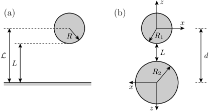
Figure 1: (a) Plane-sphere and (b) sphere-sphere geometry with the geometric parametrization used in this paper. The surface-to-surface distance is always referred to as $L$ while $\mathcal{L}$ denotes the distance between the plane and the center of the sphere and $d$ denotes the distance between the centers of the spheres.

The negative Casimir entropy for the sphere-plane geometry with perfect metals is shown in Fig. 2 as a function of the ratio of the distance $L$ between the sphere’s surface and the plane to the radius $R$ of the sphere, and of the temperature $T$. The Casimir entropy vanishes along the dashed line. Below this line, the Casimir entropy is negative while it is positive above. The grey area indicates parameter regions where the Casimir entropy has not been evaluated.

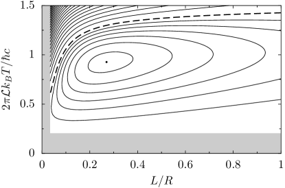
Figure 2: The Casimir entropy in the sphere-plane geometry is depicted for perfect metals as a function of the distance $L$ between sphere and plane and the temperature $T$. The entropy vanishes along the dashed line. Below this line, the entropy is negative and changes in steps of 0.0005. The minimum of the entropy is marked by a dot. Above the dashed line, the entropy is positive and changes in steps of 0.001. No data have been calculated in the grey region.

According to Fig. 2, the Casimir entropy becomes minimal at $L/R\approx 0.27$ and $2\pi\mathcal{L}k_{B}T/\hbar c\approx 0.93$. At a fixed temperature, the Casimir entropy becomes positive if the radius $R$ is sufficiently large. In contrast, for small radii, the Casimir entropy will always be negative for temperatures below a threshold value to be specified in the discussion of the free energy (4), see below.

It would be expected that the sphere-plane configuration can be obtained from the sphere-sphere configuration by letting the radius of one of the two spheres go to infinity. To illustrate this transition, we show in Fig. 3 the position of the minimum of the Casimir entropy for perfect metals as a function of the geometric parameters and the temperature for two spheres with radii $R_{<}$ and $R_{>}$ for the smaller and larger sphere, respectively. For the filled circles, the corresponding values of the ratio $R_{>}/R_{<}$ are indicated, ranging from $R_{>}/R_{<}=1$ for spheres of equal radius to the extreme case $R_{>}/R_{<}=\infty$ for which the position of the entropy minimum for the plane-sphere geometry is shown. The data clearly indicate a smooth transition between the sphere-sphere and the plane-sphere configuration.

Figure 3: The transition from perfect-metal sphere-sphere to sphere-plane configurations is illustrated by the position of the minimum of the entropy as a function of the surface-to-surface distance $L$ and the temperature $T$. The points refer to different ratios of the radii $R_{>}$ and $R_{<}$ of the larger and smaller sphere, respectively. For the filled circles, the ratio of radii is indicated in the plot. The point marked by $\infty$ corresponds to the position of the minimum of the Casimir entropy in Fig. 2.

As far as the physical origin of the negative Casimir entropy is concerned, the presentation of the data in Fig. 2 is somewhat misleading because for small sphere radius, the entropy decreases with the volume of the sphere. It is thus appropriate to scale the entropy with $(\mathcal{L}/R)^{3}$. The result is depicted in Fig. 4 where the dashed line again indicates a vanishing Casimir entropy and negative values of the Casimir entropy are found below the dashed line. Note that in this plot, in contrast to Fig. 2, small sphere radii are on the left side. The minimum of the scaled Casimir entropy lies at $R=0$. We can thus conclude that the large-distance limit $L,\mathcal{L}\gg R$ is well suited for an analysis of the negative Casimir entropy.

Figure 4: The Casimir entropy in the sphere-plane geometry multiplied by a factor $(\mathcal{L}/R)^{3}$ is displayed for perfect metals as a function of the inverse of the distance $\mathcal{L}$ between sphere’s center and the plane and the temperature $T$. The entropy vanishes along the dashed line. Below this line, the entropy is negative and changes in steps of 0.00125. Above the dashed line, the entropy is positive and changes in steps of 0.0025. No data have been calculated in the grey region.

By means of the thermodynamic relation

$$\mathcal{S}=-\frac{\partial\mathcal{F}}{\partial T}\,,$$ (3)

the Casimir entropy $\mathcal{S}$ for the sphere-plane configuration with perfect metals in the large-distance limit can easily be obtained from the expression for the Casimir free energy $\mathcal{F}$ in this limit Canaguier2010

$$\mathcal{F}=\frac{3\hbar c}{16\pi}\frac{R^{3}}{\mathcal{L}^{4}}\left[g(\nu)\cosh(\nu)+g(\nu)^{2}+g(\nu)^{3}\cosh(\nu)\right]\,,$$ (4)

where we introduced the abbreviation

$$g(\nu)=\frac{\nu}{\sinh(\nu)}\,.$$ (5)

Taking the derivative with respect to temperature, one finds negative values for the Casimir entropy for temperatures satisfying $0<\nu\lessapprox 1.486$ in agreement with the data shown in Fig. 4 for small values of $R$. In order to obtain information about the physical origin of the negative Casimir entropy, in Sect. IV.1 we will decompose the free energy (4) and the entropy derived from it into contributions arising from different scattering channels.

For the sphere-sphere geometry, the region of negative Casimir entropy for perfect-metal spheres of equal radii is displayed in Fig. 5 where the entropy is scaled by $(d/R)^{6}$. The dashed line separates the regions of negative and positive Casimir entropies with negative values appearing inside the region delimited by the dashed line. As an obvious difference to the sphere-plane geometry shown in Fig. 4 we observe that while in the latter case negative values of the Casimir entropy are found down to the lowest temperatures, this is not the case in the sphere-sphere geometry. This fact has already been noted in Rodriguez2011 . Furthermore, the region of negative Casimir entropies ends before $R/d$ reaches its maximum value of $1/2$.

Figure 5: The Casimir entropy in the sphere-sphere geometry multiplied with $(d/R)^{6}$ is depicted for perfect metals as a function of the inverse of the distance $d$ between the centers of the spheres and of the temperature $T$ for spheres of equal radii, $R_{1}=R_{2}=R$. The entropy vanishes along the dashed line. Inside the region bounded by the dashed line, the entropy is negative and changes in steps of 0.025. Outside of the dashed line, the entropy is positive and changes in steps of 0.005. The density of the contour lines has been decreased at higher temperatures to improve the clarity of the plot.

Despite these differences, Fig. 5 suggests that again interesting insights into the physics of the negative Casimir entropy can be obtained from the large-distance limit $d\gg R$. The free energy for perfect-metal spheres in this limit is given by Rodriguez2011

$$\mathcal{F} =-\frac{\hbar c}{16\pi}\frac{R^{6}}{d^{7}}\left[30g(\nu)\cosh(\nu)+30g(\nu)^{2}\right.$$ (6)

$$\qquad\qquad+29g(\nu)^{3}\cosh(\nu)+9g(\nu)^{4}\left(2\cosh(\nu)^{2}+1\right)$$

$$\,. \qquad\qquad\left.+9g(\nu)^{5}\cosh(\nu)\left(\cosh(\nu)^{2}+2\right)\right]\,,$$

where $g(\nu)$ was defined in (5). A decomposition of this result and the corresponding entropy in terms of the scattering channels will be carried out in Sect. IV.2.

III Large-distance approximation

Within the scattering approach, the Casimir free energy can be expressed as

$$\mathcal{F}=2k_{B}T\sum_{n=0}^{\infty}{}^{\prime}\sum_{m=0}^{\infty}{}^{\prime}\ln\left(\det\left[1-\mathcal{M}^{(m)}(\xi_{n})\right]\right)\,.$$ (7)

The first sum runs over the Matsubara frequencies $\xi_{n}=2\pi n/\hbar\beta$ with $\beta=1/k_{B}T$. The prime indicates that only one half of the $n=0$-term should be taken. The geometries depicted in Fig. 1 are symmetric under rotations around the $z$-axis, thus allowing us to decompose the scattering problem into subspaces of fixed eigenvalues $m$ of the $z$-component of the angular momentum. Since the sign of $m$ is irrelevant for the scattering process, we sum only over positive values of $m$, leading to a prefactor 2 except for $m=0$ as again indicated by a prime.

The matrix $\mathcal{M}^{(m)}(\xi_{n})$ describes a roundtrip scattering process between the two scattering objects at imaginary frequency $i\xi_{n}$ in the subspace of the $z$-component of the angular momentum characterized by $m$. The roundtrip scattering operator

$$\mathcal{M}^{(m)}=\mathcal{R}_{1}^{(m)}\mathcal{T}_{12}^{(m)}\mathcal{R}_{2}^{(m)}\mathcal{T}_{21}^{(m)}$$ (8)

contains four building blocks, namely the translation operator $\mathcal{T}_{21}$ from the reference frame of object 1 to that of object 2, the reflection operator $\mathcal{R}_{2}$ on object 2, the reverse translation operator $\mathcal{T}_{12}$, and finally the reflection operator $\mathcal{R}_{1}$ on object 1. While keeping the quantum number $m$ unchanged, these operators will in general modify the other parameters of the scattered modes like their polarization and, for spherical waves, their angular momentum quantum number $\ell$ or, for plane waves, their wave vector $\mathbf{k}$.

We argued in the previous section that the limit of large distances between the scattering objects is appropriate to analyze the origin of negative Casimir entropies. To be specific, we assume that the distance $D$ is much larger than the sphere radius $R$. In the case of two spheres, $R$ refers to the larger of the two radii. As we shall see now, this limit allows us to quantify the contribution of each scattering channel to the Casimir entropy.

Since the matrix elements of the translation operators for imaginary frequencies decay exponentially with $D$, the highest relevant frequencies are of the order of $c/D$. The reflection on a sphere will then contribute a factor $(R/D)^{2\ell+1}$ where $\ell$ denotes the order of the multipole wave scattered at the sphere. As a consequence, we may restrict the scattering at a sphere to $\ell=1$. In the large-distance limit, the Casimir entropy for the sphere-plane geometry and the sphere-sphere geometry thus scales with $(R/\mathcal{L})^{3}$ and $(R/d)^{6}$, respectively. These factors are at the origin of the scaling employed in the previous section.

Furthermore, in the large-distance limit the matrix elements of the roundtrip operator are very small and we may expand the logarithm in (7). In view of $\text{tr}(\mathsf{A})=\log[\det(\exp(\mathsf{A}))]$ with tr denoting the trace, we then obtain

$$\mathcal{F}=-k_{B}T\sum_{n=0}^{\infty}{}^{\prime}\sum_{P,P^{\prime}}\left[\mathcal{M}^{(0)}_{P,P}(\xi_{n})\delta_{P,P^{\prime}}+2\mathcal{M}^{(1)}_{P,P^{\prime}}(\xi_{n})\right]\,,$$ (9)

where $P$ and $P^{\prime}$ denote the polarizations on the two scattering objects. Even though we restrict our considerations to $\ell=1$ on each sphere, the translation operators $\mathcal{T}$ present in the matrix elements $\mathcal{M}^{(m)}_{P,P^{\prime}}$ implicitly give rise to a sum over other multipole moments $\ell^{\prime}$ or, in the sphere-plane geometry, to an integral over the projection $\mathbf{k}_{\parallel}$ of the wave vector onto the plane.

The polarizations $P$ and $P^{\prime}$ in (9) can be either transverse electric (TE) or transverse magnetic (TM) and correspond to the mode polarizations on the two scatterers. Note that on a sphere, the TE and TM polarizations are sometimes referred to as H and E polarizations, respectively. While in general, the polarization may change in the course of the scattering process, this is not the case for $m=0$. In this case, for a TE (TM) mode on the sphere the electric (magnetic) field will only have a component in the plane perpendicular to the $z$ direction. As a consequence, the expansion of this mode on the other sphere or the plane will contain exclusively TE (TM) modes and no polarization change ensues.

We thus have to account for three essentially different scattering channels. The channels where the polarization is conserved contribute for $m=0$ and $m=1$. A third channel involves a change of polarization and is restricted to $m=1$. The latter channel is of particular interest for our discussion for the following reason.

Focussing on the contribution of the translation operator, it is clear that in the absence of a shift, the polarization of the mode cannot change. In (9), for dimensional reasons, the shift can only appear in the combination $\xi_{n}D/c$. As a consequence, the $n=0$ term will vanish if the polarizations $P$ and $P^{\prime}$ differ, implying in turn that the free energy contribution of this channel will vanish at high temperatures. Since the contribution to the Casimir free energy of the polarization-changing channel at zero temperature is negative and turns out to be monotonically increasing, its contribution to the Casimir entropy in view of (3) will always be negative.

While the differences between the scattering channels discussed so far were mainly due to the translation operators $\mathcal{T}$, the reflection properties of the sphere(s) offer an interesting way to select channels. The reflection at a perfectly conducting (PC) sphere of radius $R$ to leading order in $\xi R/c$ is dominated by the Mie coefficients with $\ell=1$. For the TM mode, the Mie coefficient is then given by

$$a_{1}^{\text{PC}}(\xi)=-\frac{2}{3}\left(\frac{\xi R}{c}\right)^{3}+O(\xi^{5})$$ (10)

and for the TE mode it reads

$$b_{1}^{\text{PC}}(\xi)=\frac{1}{3}\left(\frac{\xi R}{c}\right)^{3}+O(\xi^{5})\,.$$ (11)

We thus have $a_{1}^{PC}=-2b_{1}^{PC}$, leading to simple numerical relations between the contributions of the polarization-conserving scattering channels.

In contrast, for spheres made of a metal described by the Drude model (D), one finds

$$a_{1}^{\text{D}}(\xi)=-\frac{2}{3}\left(\frac{\xi R}{c}\right)^{3}+O(\xi^{4})\,,$$ (12)

while $b_{1}^{\text{D}}(\xi)$ is of order $(\xi R/c)^{4}$ and therefore negligible within the large-distance approximation. Switching from a perfectly conducting sphere to a Drude metal sphere allows us to suppress the reflection of TE modes on the sphere. In particular, the polarization-changing channel will become irrelevant as we will explain in more detail in Sect. V.

These general considerations and their consequences for the Casimir entropy will be worked out more explicitly in the following section dealing with the specific geometries shown in Fig. 1.

IV Casimir free energy and entropy for perfect conductors

IV.1 Sphere-plane geometry

Within the large-distance approximation, we only need the matrix elements of the roundtrip operator for $m=0$ and $1$ to obtain the free energy by means of (9). We then can make use of (3) to obtain the entropy. For the sphere-plane geometry, the matrix element of the roundtrip operator can easily be obtained from the expressions given in Ref. Canaguier2010 . For $m=0$, we obtain

$$\mathcal{M}_{TM,TM}^{(0)}=\frac{1}{4}\left(\frac{R}{\mathcal{L}}\right)^{3}(1+2\tilde{\xi})\exp(-2\tilde{\xi})$$ (13)

and

$$\mathcal{M}_{TE,TE}^{(0)}=\frac{1}{2}\mathcal{M}_{TM,TM}^{(0)}$$ (14)

with the dimensionless frequency $\tilde{\xi}$ introduced in (2).

For $m=1$, the matrix elements for the roundtrips where polarization is conserved are

$$\mathcal{M}_{TM,TM}^{(1)}=\frac{1}{8}\left(\frac{R}{\mathcal{L}}\right)^{3}(1+2\tilde{\xi}+2\tilde{\xi}^{2})\exp(-2\tilde{\xi})$$ (15)

and

$$\mathcal{M}_{TE,TE}^{(1)}=\frac{1}{2}\mathcal{M}_{TM,TM}^{(1)}\,.$$ (16)

For roundtrips involving a change of polarization, one finds

$$\mathcal{M}_{TM,TE}^{(1)}=\frac{1}{4}\left(\frac{R}{\mathcal{L}}\right)^{3}\tilde{\xi}^{2}\exp(-2\tilde{\xi})$$ (17)

and

$$\mathcal{M}_{TE,TM}^{(1)}=\frac{1}{2}\mathcal{M}_{TM,TE}^{(1)}\,.$$ (18)

Here, the first subscript of the roundtrip operator $\mathcal{M}$ refers to the polarization on the sphere while the second subscript indicates the polarization on the plane. The matrix elements (17) and (18) for scattering processes involving a change of polarization vanish in the limit of vanishing frequency $\tilde{\xi}$ as discussed in the previous section.

Making use of (9), we can decompose the Casimir free energy for perfect metal sphere and plane into contributions from the different scattering channels according to

$$\mathcal{F} =-\frac{\hbar c}{2\pi\mathcal{L}}\left(\frac{R}{\mathcal{L}}\right)^{3}\left[f^{(0)}_{TM,TM}+f^{(0)}_{TE,TE}\right.$$ (19)

$$\qquad\left.+f^{(1)}_{TM,TM}+f^{(1)}_{TE,TE}+f^{(1)}_{TM,TE}+f^{(1)}_{TE,TM}\right]\,.$$

Evaluating the corresponding Matsubara sums, we find for $m=0$ from (13)

$$f^{(0)}_{TM,TM}=\frac{1}{8}\left[g(\nu)\cosh(\nu)+g(\nu)^{2}\right]\,.$$ (20)

Here, we have made use of the dimensionless temperature (1) and the function $g$ defined in (5). For $m=1$, we obtain from (15) and (17)

$$f^{(1)}_{TM,TM}=\frac{1}{8}\left[g(\nu)\cosh(\nu)+g(\nu)^{2}+g(\nu)^{3}\cosh(\nu)\right]$$ (21)

and

$$f^{(1)}_{TM,TE}=\frac{1}{8}g(\nu)^{3}\cosh(\nu)\,,$$ (22)

respectively. The remaining three contributions in (19) are related to the expressions just given by a factor of 1/2 according to the relations (14), (16), and (18). Summing up all terms, we recover the free energy (4) for sphere and plane made of perfect conductors obtained earlier in Ref. Canaguier2010 . The decomposition in terms of the different scattering channels is found to be in agreement with the expressions obtained in Ref. Milton2014 . In order to make the connection, one sets the electric and magnetic polarizability equal to $R^{3}$ and $-R^{3}/2$, respectively. For vanishing polarizability in the transverse direction, one finds the contribution for $m=0$ while an isotropic polarizability yields the sum of the contributions from $m=0$ and $1$.

It is now straightforward to obtain the contributions of the various scattering channels to the Casimir entropy. Expressing the Casimir entropy in terms of a rescaled Casimir entropy $s$ according to

$$S=k_{B}\left(\frac{R}{\mathcal{L}}\right)^{3}s\,,$$ (23)

the definition of the entropy (3) turns into

$$s=\frac{\partial f}{\partial\nu}\,.$$ (24)

We then obtain from (20), (21), and (22)

$$s^{(0)}_{TM,TM}=\frac{1}{8\nu}\left[g(\nu)\cosh(\nu)+g(\nu)^{2}-2g(\nu)^{3}\cosh(\nu)\right]$$ (25)

$$s^{(1)}_{TM,TM} =\frac{1}{8\nu}\left[g(\nu)\cosh(\nu)+g(\nu)^{2}+g(\nu)^{3}\cosh(\nu)\right.$$ (26)

$$\qquad\qquad\left.-g(\nu)^{4}\big{(}2\cosh^{2}(\nu)+1\big{)}\right]$$

$$s^{(1)}_{TM,TE}=\frac{1}{8\nu}\left[3g(\nu)^{3}\cosh(\nu)-g(\nu)^{4}\big{(}2\cosh^{2}(\nu)+1\big{)}\right]\,.$$ (27)

The remaining three contributions to the Casimir entropy can be obtained by simple multiplication with a factor $1/2$ as before for the free energy and the matrix elements of the roundtrip operator.

In Fig. 6, the temperature dependence of the contributions (25), (26), and (27) from the channels with TM polarization on the sphere to the Casimir entropy are shown. Among the polarization-conserving channels, the $m=0$ contribution is positive for all temperatures. The $m=1$ contribution, while being slightly negative at sufficiently small temperatures, in combination with the $m=0$ contribution will still always lead to positive values of the entropy. In order to arrive at a negative entropy, one needs the polarization-changing mode. In fact, $S^{(1)}_{TM,TE}$ is negative for all temperatures as was already conjectured in Sect. III.

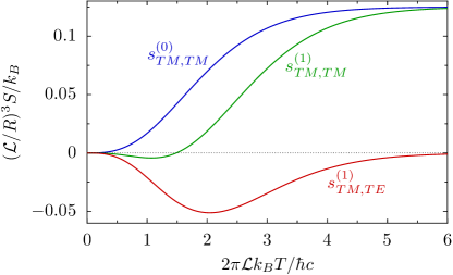
Figure 6: The contributions (25), (26), and (27) to the Casimir entropy in the plane-sphere geometry arising from the scattering channels with TM polarization on the sphere are shown as a function of the dimensionless temperature. While $S^{(0)}_{TM,TM}$ is always positive and $S^{(1)}_{TM,TM}$ becomes only slightly negative for small temperatures, $S^{(1)}_{TM,TE}$ is negative for all temperatures.

The negative contribution of the polarization-changing channel is indeed sufficiently large to render the sum of all contributions negative. This can clearly be seen from the low-temperature expansions of the entropies (25)–(27)

$$s^{(0)}_{TM,TM} =\frac{1}{45}\nu^{3}-\frac{2}{315}\nu^{5}+O(\nu^{7})$$ (28)

$$s^{(1)}_{TM,TM} =-\frac{1}{90}\nu^{3}+\frac{1}{105}\nu^{5}+O(\nu^{7})$$ (29)

$$s^{(1)}_{TM,TE} =-\frac{1}{30}\nu^{3}+\frac{1}{63}\nu^{5}+O(\nu^{7})\,.$$ (30)

Taking all six channels between perfect conductor plane and sphere into account, we obtain for the low-temperature expansion of the Casimir entropy

$$s=-\frac{1}{30}\nu^{3}+\frac{1}{35}\nu^{5}+O(\nu^{7})\,.$$ (31)

In the large-distance limit, we thus obtain negative values for the Casimir entropy at sufficiently low temperatures. In the limit of vanishing temperature, the Casimir entropy goes to zero in agreement with the third law of thermodynamics.

IV.2 Sphere-sphere geometry

We now turn to the discussion of the Casimir free energy and entropy of the sphere-sphere configuration depicted in Fig. 1b. In order to determine the Casimir free energy in the limit of large distance, $d\gg R_{1},R_{2}$, from the expression (9), we first need to determine the matrix elements $\mathcal{M}^{(m)}_{P,P^{\prime}}$ of the round-trip operator with $m=0$ and $1$.

As discussed in Sect. III, the large-distance approximation implies that on the spheres, we can restrict the field modes to dipole spherical waves, $\ell=1$. For the spheres, the matrix elements of the reflection operators are thus simply given by the Mie coefficients (10) and (11), and we have

$$\mathcal{R}^{(m)}_{TM,TM}=-\frac{2}{3}\left(\frac{R}{d}\right)^{3}\tilde{\xi}^{3}$$ (32)

and

$$\mathcal{R}^{(m)}_{TE,TE}=\frac{1}{3}\left(\frac{R}{d}\right)^{3}\tilde{\xi}^{3}\,,$$ (33)

where $R$ is the sphere radius and $\tilde{\xi}$ is the dimensionless imaginary frequency (2). In contrast to the reflection on a plane in the preceding subsection, the polarization of a spherical wave remains unchanged by the reflection at a sphere.

However, the translation operator for spherical waves with wave vector $k$ from the center of one sphere to the center of the other sphere leads to a mixing of polarizations. The general expressions for the matrix elements of the translation operator Cruzan1962 can be simplified if the translation is performed along the $z$-axis Bruning1969 ; Bruning1971 as is the case in the setup displayed in Fig. 1b. Within the large-distance approximation, we find for the channels conserving the polarization

$$\mathcal{T}^{(m)}_{P,P} =(-1)^{m}\frac{3}{4}\sum_{\ell^{\prime}=0,2}i^{-\ell^{\prime}}[4-\ell^{\prime}(\ell^{\prime}+1)](2\ell^{\prime}+1)$$ (34)

$$\qquad\times\begin{pmatrix}1&1&\ell^{\prime}\\ 0&0&0\end{pmatrix}\begin{pmatrix}1&1&\ell^{\prime}\\ m&-m&0\end{pmatrix}h_{\ell^{\prime}}^{(1)}(kd)\,.$$

For a change of polarization, $P\neq P^{\prime}$, the matrix element vanishes for $m=0$ in agreement with the argument given in Sect. III, while for $m=1$ we have

$$\mathcal{T}^{(1)}_{P,P^{\prime}} =\pm\frac{3}{2}ikd\sum_{\ell^{\prime}=0,2}i^{-\ell^{\prime}}(2\ell^{\prime}+1)$$ (35)

$$\qquad\times\begin{pmatrix}1&1&\ell^{\prime}\\ 0&0&0\end{pmatrix}\begin{pmatrix}1&1&\ell^{\prime}\\ 1&-1&0\end{pmatrix}h_{\ell^{\prime}}^{(1)}(kd)\,.$$

The first two factors in the second lines of (34) and (35) denote Wigner $3j$ symbols while $h_{\ell}^{(1)}$ is a spherical Bessel function of the third kind. The overall sign in (35) is positive or negative depending on whether the translation is performed in positive or negative $z$-direction, respectively.

Employing the relation

$$h_{\ell}^{(1)}(ix)=-\frac{2}{\pi}i^{-\ell}k_{\ell}(x)$$ (36)

between the spherical Bessel function of the third kind and the modified spherical Bessel function $k_{\ell}$, it is straightforward to express the matrix elements of the translation operator in imaginary frequency $\xi$ needed in order to evaluate the Matsubara sum (9). With the explicit expressions for the modified spherical Bessel functions

$$k_{0}(x) =\frac{\pi}{2}\frac{\exp(-x)}{x}$$ (37)

$$k_{2}(x) =\frac{\pi}{2}\left(\frac{1}{x}+\frac{3}{x^{2}}+\frac{3}{x^{3}}\right)\exp(-x)$$

the matrix elements needed in the following are then found to read

$$\mathcal{T}^{(0)}_{P,P}=3\left(\frac{1}{\tilde{\xi}^{3}}+\frac{1}{\tilde{\xi}^{2}}\right)\exp(-\tilde{\xi})$$ (38)

and

$$\mathcal{T}^{(1)}_{P,P}=-\frac{3}{2}\left(\frac{1}{\tilde{\xi}^{3}}+\frac{1}{\tilde{\xi}^{2}}+\frac{1}{\tilde{\xi}}\right)\exp(-\tilde{\xi})$$ (39)

for $P=TE,TM$ while for differing polarizations $P$ and $P^{\prime}$ one finds

$$\mathcal{T}^{(1)}_{P,P^{\prime}}=\pm\frac{3}{2}\left(\frac{1}{\tilde{\xi}^{2}}+\frac{1}{\tilde{\xi}}\right)\exp(-\tilde{\xi})\,.$$ (40)

In the last equation, the sign depends on the direction of translation with respect to the $z$-axis as discussed in the context of (35).

We note that even though these matrix elements diverge for vanishing frequency $\tilde{\xi}$, their products with the matrix elements (32) and (33) of the reflection operator remain finite. While the combination of the two matrix elements yields a nonzero value if the polarization is conserved, the product of the matrix element (40) for changing polarization with one of the reflection matrix elements (32) and (33) goes to zero for vanishing frequency $\tilde{\xi}$.

As a consequence, the contribution of the polarization-changing channels to the Casimir free energy and entropy vanishes at high temperatures where the Matsubara sum (9) is dominated by the $n=0$ term. Already at this point, we can therefore expect the same qualitative temperature dependence of the contributions of the polarization-changing channels as in the plane-sphere geometry. These channels will thus play the same crucial role for an overall negative Casimir entropy also for the sphere-sphere geometry. The difference between the polarization-conserving and polarization-changing channels can be traced back to an extra factor $kd$ appearing in the front of the right-hand side of (35) compared to (34). This factor ensures that for vanishing translation, $d=0$, no change of polarization occurs as was argued in Sect. III.

With the matrix elements listed above, it is straightforward to evaluate the contributions of the various channels to the Casimir free energy by means of (8) and (9). We decompose the Casimir free energy into the contributions from the various scattering channels

$$\mathcal{F} =-\frac{\hbar c}{2\pi d}\left(\frac{R_{1}R_{2}}{d^{2}}\right)^{3}\left[f^{(0)}_{TM,TM}+f^{(0)}_{TE,TE}\right.$$ (41)

$$\qquad\left.+f^{(1)}_{TM,TM}+f^{(1)}_{TE,TE}+f^{(1)}_{TM,TE}+f^{(1)}_{TE,TM}\right]\,.$$

The contributions to (41) arising from polarization-conserving channels are given by

$$f^{(0)}_{TM,TM}=2g(\nu)\cosh(\nu)+2g(\nu)^{2}+g(\nu)^{3}\cosh(\nu)$$ (42)

and

$$f^{(1)}_{TM,TM} =\frac{1}{2}\left[2g(\nu)\cosh(\nu)+2g(\nu)^{2}+3g(\nu)^{3}\cosh(\nu)\right.$$ (43)

$$\qquad\quad+g(\nu)^{4}\big{(}2\cosh^{2}(\nu)+1\big{)}$$

$$\qquad\quad\left.+g(\nu)^{5}\cosh(\nu)\big{(}\cosh^{2}(\nu)+2\big{)}\right]$$

together with

$$f^{(m)}_{TE,TE}=\frac{1}{4}f^{(m)}_{TM,TM}\,.$$ (44)

The contributions of the polarization-changing channels are

$$f^{(1)}_{TM,TE} =\frac{1}{4}\left[g(\nu)^{3}\cosh(\nu)+g(\nu)^{4}\big{(}2\cosh^{2}(\nu)+1)\right.$$ (45)

$$\qquad\quad\left.+g(\nu)^{5}\cosh(\nu)\big{(}\cosh^{2}(\nu)+2\big{)}\right]$$

and

$$f^{(1)}_{TE,TM}=f^{(1)}_{TM,TE}\,.$$ (46)

In these results, we make use of the dimensionless temperature (1) and the function $g$ defined in (5). The total Casimir free energy obtained from these expressions agrees with the result (6) and was already given in Ref. Rodriguez2011 . As in the sphere-plane geometry, the contributions from the different scattering channels are in agreement with the results presented in Ref. Milton2014 if the identifications explained above are made.

In the high-temperature limit, $\nu\to\infty$, the polarization-conserving channels yield a contribution to the Casimir free energy linear in temperature while the contributions of the polarization-changing channels vanish. On the other hand, all channels give rise to a negative Casimir free energy at zero temperature. As a consequence, the contribution to the Casimir entropy arising from the polarization-changing channels is negative for all temperatures as already expected above on the basis of the matrix elements of the translation operator.

From the expressions listed for the contributions to the Casimir free energy, the corresponding contributions to the Casimir entropy can be obtained from its definition (3). Introducing a rescaled Casimir entropy $s$ by means of

$$S=k_{B}\left(\frac{R_{1}R_{2}}{d^{2}}\right)^{3}s\,,$$ (47)

one finds together with the abbreviation (5)

$$s^{(0)}_{TM,TM} =\frac{1}{\nu}\left[2g(\nu)\cosh(\nu)+2g(\nu)^{2}-g(\nu)^{3}\cosh(\nu)\right.$$ (48)

$$\qquad\quad\left.-g(\nu)^{4}\big{(}2\cosh^{2}(\nu)+1\big{)}\right]$$

$$=4s^{(0)}_{TE,TE}$$

$$s^{(1)}_{TM,TM} =\frac{1}{2\nu}\left[2g(\nu)\cosh(\nu)+2g(\nu)^{2}+5g(\nu)^{3}\cosh(\nu)\right.$$ (49)

$$\qquad\quad+g(\nu)^{4}\big{(}2\cosh^{2}(\nu)+1\big{)}$$

$$\qquad\quad+g(\nu)^{5}\cosh(\nu)\big{(}\cosh^{2}(\nu)+2\big{)}$$

$$\qquad\qquad\left.-g(\nu)^{6}\big{(}2\cosh^{4}(\nu)+11\cosh^{2}(\nu)+2\big{)}\right]$$

$$=4s^{(1)}_{TE,TE}$$

$$s^{(1)}_{TM,TE} =\frac{1}{4\nu}\left[3g(\nu)^{3}\cosh(\nu)+3g(\nu)^{4}\big{(}2\cosh^{2}(\nu)+1\big{)}\right.$$ (50)

$$\qquad\quad+g(\nu)^{5}\cosh(\nu)\big{(}\cosh^{2}(\nu)+2\big{)}$$

$$\qquad\quad\left.-g(\nu)^{6}\big{(}2\cosh^{4}(\nu)+11\cosh^{2}(\nu)+2\big{)}\right]$$

$$=s^{(0)}_{TE,TM}\,.$$

The temperature dependence of the contributions (48)–(50) to the Casimir entropy is shown in Fig. 7. At first sight, the curves resemble those presented in Fig. 6. In both cases, the contribution for $m=0$ is positive for all temperatures while the polarization-conserving contribution for $m=1$ starts out negative and becomes positive at higher temperatures. The polarization-changing channels always yield a negative contribution to the Casimir entropy. A closer look reveals that, in contrast to the plane-sphere configuration, the negative contribution of the polarization-conserving channel with $m=1$ at low temperatures is much bigger than the contribution of the polarization-changing channel. However, as the dashed curve in Fig. 7 shows, the sum of the Casimir entropies of the polarization-conserving channels remains positive at all temperatures.

Figure 7: The contributions (48), (49), and (50) to the Casimir entropy of a sphere-sphere configuration are depicted as a function of the dimensionless temperature. While $S^{(0)}_{TM,TM}$ is positive for all temperatures and $S^{(1)}_{TM,TM}$ can be positive or negative depending on temperature, $S^{(1)}_{TM,TE}$ always yields a negative contribution to the Casimir entropy. The dashed line represents the sum of the contributions of the two polarization-conserving transverse magnetic channels.

In order to analyze in more detail the negative contributions to the Casimir entropy, we consider the low-temperature expansions of the expressions (48)–(50) which are given by

$$s^{(0)}_{TM,TM} =\frac{4}{45}\nu^{3}+\frac{8}{315}\nu^{5}-\frac{8}{525}\nu^{7}+O(\nu^{9})$$ (51)

$$s^{(1)}_{TM,TM} =-\frac{4}{45}\nu^{3}+\frac{2}{45}\nu^{5}-\frac{68}{1575}\nu^{7}+O(\nu^{9})$$ (52)

$$s^{(1)}_{TM,TE} =-\frac{1}{63}\nu^{5}-\frac{2}{225}\nu^{7}+O(\nu^{9})\,.$$ (53)

The dominant low-temperature contributions of order $T^{3}$ arise in the polarization-conserving channels. However, they cancel each other. In view of the fact that according to (31), the Casimir entropy in the plane-sphere configuration contains a leading term of order $T^{3}$, this may come as a surprise. Indeed, a leading cubic term in the temperature can be obtained for anisotropic objects Milton2014 . For the isotropic case considered here, it can be shown that terms of order $\xi^{5}$ in the Mie coefficients (10) and (11) lead to such a $T^{3}$ term in the sphere-sphere configuration. However, this term is suppressed by a factor of $(R/d)^{3}$ relative to the terms discussed here and therefore negligible in the large-distance limit.

With the order $T^{3}$ not contributing to the entropy, the appearance of a negative Casimir entropy is a nonperturbative effect Milton2014 . In the next order, $T^{5}$, the negative contribution of the polarization-changing channel is not sufficiently strong as compared to the positive contributions of that order. Therefore, at very low temperatures, the Casimir entropy of two perfectly conducting spheres will be positive. On the other hand, it turns out that the terms of order $T^{7}$, which in (51)–(53) are all negative, lead indeed to a negative Casimir entropy in an intermediate temperature range. This was already shown in Ref. Rodriguez2011 and is also visible in Fig. 5.

It is now interesting to study how the different channels can contribute in various ways to obtain either a positive Casimir entropy for all temperatures or a negative Casimir entropy in a certain temperature regime. To this end, in the next section we will also allow for spheres made of Drude-type metals.

V Perfectly conducting vs. Drude-type metal spheres

So far, we have studied the behavior of the various scattering channels and pointed out the relevance of the polarization-changing channels for the appearance of a negative Casimir entropy. The weight with which the scattering channels contribute can be modified by the physical properties of the objects involved. In Ref. Milton2014 this was done by choosing objects with anisotropic polarizabilities and by varying their electric and magnetic properties. Here, we will do the latter by allowing the objects to be either made of perfectly conducting metals or Drude-type metals which have a finite zero-frequency conductivity. The results will further underline the relevance of the polarization-changing channels.

For simplicity, we will restrict ourselves in the following to setups consisting of two spheres as depicted in Fig. 1b. Then, as pointed out in Sect. IV.2, the matrix elements of the reflection operator are given by the Mie coefficients for $\ell=1$. While for perfectly conducting spheres, the Mie coefficients are the same up to a factor -2, for Drude metal spheres with a dc conductivity $\sigma_{0}$, the reflection of the TE mode can be neglected in the large-distance limit where in addition to the conditions stated earlier, $d\gg\sigma_{0}R^{2}/30c$ should hold.

These properties of the Mie coefficients allow us to construct three different scenarios by choosing two spheres both made of perfect conductors, both made of Drude metals, or one made of a perfect conductor and the other of a Drude metal. In the first case, polarization-conserving as well as polarization-changing channels contribute as discussed in Sect. IV.2. In contrast, in the second case, only modes with TM polarization can complete roundtrips between the two spheres. Therefore, in this case, the polarization-changing channel is completely suppressed. In the third case, only one of the two polarization-changing channels and its weight relative to the polarization-conserving channels is modified with respect to two perfectly conducting spheres.

Indicating in the superscript on the left-hand side the material of which the two spheres are made, we obtain for the three situations just described the rescaled entropy introduced in (47) with

$$s^{\text{PC/PC}} =\frac{5}{4}\left(s^{(0)}_{TM,TM}+s^{(1)}_{TM,TM}\right)+2s^{(1)}_{TM,TE}$$ (54)

$$s^{\text{PC/D}} =s^{(0)}_{TM,TM}+s^{(1)}_{TM,TM}+s^{(1)}_{TM,TE}$$ (55)

$$s^{D/D} =s^{(0)}_{TM,TM}+s^{(1)}_{TM,TM}\,,$$ (56)

where the components are given in (48)–(50). These results are consistent with those obtained in Ref. Milton2014 .

The temperature dependence of the Casimir entropies (54)–(56) is displayed in Fig. 8. At high temperatures, only the polarization-conserving channels contribute. The difference between the case of perfectly conducting spheres and the other two cases shows the suppression of the polarization-conserving TE channel due to a Drude metal sphere.

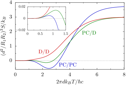
Figure 8: Temperature dependence of the Casimir entropies (54)–(56) for a sphere-sphere setup where the spheres are either made of perfect conductors (PC) or Drude metals (D). The inset shows the low-temperature behavior where a positive Casimir entropy is found for all three cases. The curve for D/D corresponds to the dashed curve in Fig. 7.

The inset puts a special emphasis on the low-temperature behavior and shows clearly that in all three cases, the Casimir entropy takes on positive values for very low temperatures. However, only when all spheres are made of a Drude metal does the Casimir entropy remain positive for all temperatures. This is the case where no polarization-changing channels contribute.

It is sufficient to allow for one polarization-changing channel by making one of the spheres perfectly conducting in order to obtain a temperature window in which the Casimir entropy becomes negative. The effect becomes even more pronounced if both spheres are perfectly conducting as the weight of the polarization-changing channels is doubled while the contribution of the polarization-conserving channels is only increased by a quarter.

VI Conclusions

The origin of the negative Casimir entropy in the plane-sphere and sphere-sphere configuration has been analyzed in the limit where the distance between the objects is much larger than the radius of the sphere(s). In this limit, the Casimir free energy and the Casimir entropy can easily be decomposed into the contributions from various channels describing a roundtrip between the objects. Three kinds of channels have been identified, differing significantly in the temperature dependence of their contribution to the Casimir entropy.

The first kind of channels always makes a positive contribution to the Casimir entropy. This was found to be the case for polarization-conserving channels describing spherical waves with $m=0$.

The second kind of channels also conserves polarization but involves spherical waves with $m=1$. While these channels yield a positive contribution to the Casimir entropy at high temperatures, their contribution at sufficiently low temperatures is negative. However, this negative part is compensated by the polarization-conserving channels with $m=0$.

The third kind of channels is the most interesting one, because its contribution to the Casimir entropy is negative for all temperatures. This behavior is associated with polarization-changing channels which exist for $m=1$ but not for $m=0$. These channels are special, because their Casimir free energy vanishes in the high-temperature limit. This fact and the ensuing negative contribution to the Casimir entropy has been traced back to the polarization-changing nature of the channels. It can thus be concluded that polarization mixing in a scattering process is a crucial ingredient for the appearance of a negative Casimir entropy, at least in the plane-sphere and sphere-sphere configuration.

Which of the various channels contribute to the Casimir entropy can be influenced by appropriately choosing the material out of which the scattering objects are made. One can use the fact that in the long-distance limit the reflection of transverse electric modes at spheres made of a Drude metal becomes negligible. We have shown that for two Drude metal spheres, the Casimir entropy is positive for all temperatures. In this situation, only roundtrip scattering processes involving transverse magnetic modes are relevant. As soon as at least one of the spheres is perfectly conducting, polarization-changing processes occur and the Casimir entropy is found to become negative in a certain temperature window.

- (1) H. B. G. Casimir, Proc. K. Ned. Akad. Wet. 51, 793 (1948).
- (2) V. B. Bezerra, G. L. Klimchitskaya, and V. M. Mostepanenko, Phys. Rev. A 66, 062112 (2002).
- (3) M. Boström and B. E. Sernelius, Physica A 339, 33 (2004).
- (4) V. B. Bezerra, G. L. Klimchitskaya, V. M. Mostepanenko, and C. Romero, Phys. Rev. A 69, 022119 (2004).
- (5) I. Brevik, J. B. Aarseth, J. S. Høye, and K. A. Milton, in Proceedings of the Sixth Workshop on Quantum Field Theory Under the Influence of External Conditions, edited by K. A. Milton (Rinton Press, Princeton, 2004), pp. 54–65.
- (6) I. Brevik, J. B. Aarseth, J. S. Høye, and K. A. Milton, Phys. Rev. E 71, 056101 (2005).
- (7) V. B. Svetovoy and R. Esquivel, Phys. Rev. E 72, 036113 (2005).
- (8) I. Brevik, J. B. Aarseth, J. S. Høye, and K. A. Milton, Phys. Rev. E 71, 056101 (2005).
- (9) V. B. Bezerra, G. L. Klimchitskaya, V. M. Mostepanenko, and C. Romero, Phys. Rev. A 78, 042901 (2008).
- (10) S. Å. Ellingsen, I. Brevik, J. S. Høye, and K. A. Milton, J. Phys.: Conf. Ser. 161, 012010 (2009).
- (11) G.-L. Ingold, A. Lambrecht, and S. Reynaud, Phys. Rev. E 80, 041113 (2009).
- (12) L. P. Pitaevskii, in Quantum Field Theory Under the Influence of External Conditions (QFEXT09), edited by K. A. Milton and M. Bordag (World Scientific, Singapore, 2010), p. 227.
- (13) A. Canaguier-Durand, P. A. Maia Neto, A. Lambrecht, and S. Reynaud, Phys. Rev. A 82, 012511 (2010).
- (14) M. Bordag and I. G. Pirozhenko, Phys. Rev. D 82, 125016 (2010).
- (15) R. Zandi, T. Emig, and U. Mohideen, Phys. Rev. B 81, 195423 (2010).
- (16) A. Weber and H. Gies, Phys. Rev. D 82, 125019 (2010).
- (17) P. Rodriguez-Lopez, Phys. Rev. B 84, 075431 (2011).
- (18) K. A. Milton, R. Guérout, G.-L. Ingold, A. Lambrecht, S. Reynaud, to appear in J. Phys.: Condens. Matter.
- (19) O. R. Cruzan, Quart. Appl. Math. 20, 33 (1962).
- (20) J. H. Bruning and Y. T. Lo, Tech. Rep. 69-5 (Antenna Lab, Urbana Illinois, 1969).
- (21) J. H. Bruning and Y. T. Lo, IEEE Trans. Ann. Prop. 19, 378 (1971).