Bound states on the lattice with partially twisted boundary conditions

Abstract

We propose a method to study the nature of exotic hadrons by determining the wave function renormalization constant $Z$ from lattice simulations. It is shown that, instead of studying the volume-dependence of the spectrum, one may investigate the dependence of the spectrum on the twisting angle, imposing twisted boundary conditions on the fermion fields on the lattice. In certain cases, e.g., the case of the $DK$ bound state which is addressed in detail, it is demonstrated that the partial twisting is equivalent to the full twisting up to exponentially small corrections.

I Introduction

The search for the exotic states (tetraquarks, hybrids, hadronic molecules, etc) in the observed hadron spectrum has been a subject of both theoretical and experimental investigations for decades. The exact pattern, how these states emerge, should be strictly determined by the underlying theory and should therefore contain important information about the behavior of QCD at low energies. In practice, however, extracting such information from the data encounters certain challenges, which are in part of a conceptual nature. In the present paper we wish to focus exactly on this issue.

In general, a state is called “exotic” if its quark content does not correspond to the “standard” constellation given by the non-relativistic quark model ($q\bar{q}$ for mesons and $qqq$ for baryons). Consequently, one needs to use a particular model as a reference point to define how the exotic states are meant (note that the very notion of constituent quarks is, strictly speaking, model-dependent). Putting it differently, one has to agree on certain criteria formulated in terms of certain hadronic observables: if these observables are measured, or calculated on the lattice, and the results do not follow the pattern predicted by the quark model, this then should be interpreted as a signature for exotica.

A standard example for the exotic state candidates is given by the scalar nonet with the masses around 1 GeV. As it is well known, the observed mass hierarchy in this nonet is reversed as compared to, e.g., the pseudoscalar or vector multiplets. Such a mass ordering is counter-intuitive from the point of view of the naive quark model, but can be easily understood, if the scalar mesons were interpreted as tetraquark states (see, e.g., Jaffe:1976ig ; Black:1998wt ; Achasov:2002ir ; Pelaez:2004xp ). This is, however, not the only possible interpretation. In Refs. Weinstein:1982gc ; Oller:1997ng ; Oller:1998hw , the $a_{0}(980)$ and $f_{0}(980)$ were considered as hadronic molecules, whereas in Refs. Oller:1998zr these states were described as a combination of a bare pole and the rescattering contribution. In the Jülich meson-exchange model, the $f_{0}(980)$ appears to be a bound $K\bar{K}$ state, whereas the $a_{0}(980)$ is a dynamically generated threshold effect Janssen:1994wn . Similar conclusions were inferred in Ref. Guo:2011pa from the calculations in the unitarized ChPT with explicit resonance states. Finally, the investigations carried out within the framework of QCD sum rules are also indicative of the non-$q\bar{q}$ nature of $a_{0}(980)$ sumrules . Given these multiple interpretations, it is natural to look for the clear-cut criteria based on the observables in order to minimize the model-dependence of the statements about the nature of the hadronic states in question.

In fact, such criteria are known for quite some time already. The “pole counting” method, considered in Refs. Morgan:1992ge ; Tornqvist:1994ji , relates the number of the $S$-matrix poles near threshold to the molecular nature of the states corresponding to these poles. Namely, it has been argued that the loosely bound states of hadrons (hadronic molecules) correspond to a single pole, whereas the poles corresponding to the tightly bound quark states (of standard or exotic nature) always come in pairs. A closely related criterion goes under the name of Weinberg’s compositeness condition Weinberg , which uses the quantity called the wave function renormalization constant $Z$, where $0\leq Z\leq 1$, to differentiate between the loosely bound states and tight QCD composites, the values $Z\simeq 0$ corresponding to the molecular states and vice versa. The application of these methods for the analysis of the data on scalar mesons are considered in Refs. Morgan:1993td ; Baru:2003qq ; Baru:2004xg ; Hanhart:2006nr ; Hanhart:2007cm ; Hyodo:2011qc , and the recent review on the subject may be found in Ref. Hyodo:2013nka . Moreover, theoretically, one may study the dependence of the pole positions on the number of the colors $N_{c}$ (see Refs. Nebreda:2011cp ; Guo:2011pa ; Pelaez:2006nj ) or the quark masses (Refs. Hanhart:2008mx ; Pelaez:2010fj ; Bernard:2010fp ; Albaladejo:2012te ). From the above studies, one can judge about the precise structure of these states beyond the simple alternative between a molecule and a tight quark composite.

Recent years have seen a renewed interest in the field, which is partly related to the progress in the lattice calculations of the QCD spectrum at the quark masses close to the physical values. It should be realized that the lattice studies have powerful tools at their disposal to analyze the nature of the states that emerge in QCD. Apart from the information about the dependence of the spectrum on quark masses, a valuable information comes from the volume dependence of the calculated spectrum as well as its dependence on the twisting angle in case of twisted boundary conditions, see Refs. Suganuma:2005ds ; MartinezTorres:2011pr ; Sekihara:2012xp ; Ozaki:2012ce ; Albaladejo:2013aka . Note that all this information is obtained from the first-principle calculations on the lattice and is thus in principle devoid of any model-dependent input.

In this paper we investigate the nature of the scalar states in the sector with one charm quark that is a natural generalization of our treatment of the light scalar mesons. We mainly focus on the case of the $D_{s0}^{*}(2317)$ meson experiment , albeit the formalism, which we develop here, can be straightforwardly applied to the other cases where a bound state close to the elastic threshold emerges (note that, in this paper, we do not consider the generalization of the approach to the inelastic case. This forms a subject of a separate investigation.). The $D_{s0}^{*}(2317)$ does not fit very nicely to the quark-model picture, and its structure is still debated, see, e.g., Ref. Zhu:2007wz for a recent review. The molecular picture, due to the closeness of the $DK$ threshold and a large coupling to the $DK$ channel looks most promising among other alternatives. It would be highly desirable to verify this conjecture in a model-independent manner, on the basis of the lattice calculations. To this end, one may use the fact that the dependence of the bound-state energy on the kaon mass is very different for a molecule and a standard quark-model state, see Ref. Cleven . Another possible method to address this issue has been described, e.g., in Refs. MartinezTorres:2011pr ; Sekihara:2012xp , where the authors propose to study the volume-dependence of the spectrum in order to apply the Weinberg’s compositeness criterion on the lattice.

The exploratory study of light pseudoscalar mesons $(\pi,K)$ of $(D,D_{s})$ in full lattice QCD has been carried out in Refs. Liu:2012zya ; Moir:2013yfa ; prelovsek . In some isospin channels the study is plagued by the presence of disconnected contributions. The implementation of the method from Refs. MartinezTorres:2011pr ; Sekihara:2012xp , which implies carrying out calculations at different volumes, could be therefore quite expensive. In this paper we propose an alternative, which requires calculations at one volume, albeit with twisted boundary conditions. Moreover, we show that, in the study of $D_{s0}^{*}(2317)$, one may use partially twisted boundary conditions, despite the fact that the quark annihilation diagrams are present. The method used in the proof is the same as in Ref. Agadjanov:2013kja . Generally, one may expect that the simulations with partially twisted boundary conditions could be less expensive than working at different volumes, while they provide us the same information about the nature of the bound states in question.

This article is organized as follows. In Sect. II, we briefly review Weinberg’s argument for the compositeness of particles. In Sect. III we describe the procedure of extraction of the parameter $Z$ from the data with twisted boundary condition. Further, in Sect. IV we use some models and produce synthetic lattice data in order to check the procedure of the extraction in practice. The error analysis has also been carried out. Separately, in Sect. V, we discuss the use of the partially twisted boundary conditions and show that they are equivalent to the full twisting in our case. Sect. VI contains our conclusions.

II Compositeness of bound states

As mentioned before, in view of the plethora of candidates of exotic hadrons, it is very important to make model-independent statements on the nature of these states. Model-independence requires that we can only study the physical observables which can be defined in terms of the matrix elements between asymptotic states. In particular, we would like to ask a question, whether a given particle, corresponding to the $S$-matrix pole, can be regarded as “elementary” or rather as a bound state (molecule) of other hadrons. The central place in this identification belongs to the so-called wave function renormalization constant $Z$, which has been used to distinguish composite particles from elementary ones since the early 1960’s Howard ; Vaughan ; Salam:1962ap ; Weinberg:1962hj ; Weinberg ; WeinbergBook . To see its role, we will first discuss a non-relativistic quantum mechanical system, following the discussion of Ref. Weinberg .

In this section, we will restrict our discussion to the infinite volume. Let us consider a two-body system with a Hamiltonian $\mathcal{H}=\mathcal{H}_{0}+V$, where $\mathcal{H}_{0}$ is the free Hamiltonian, and $V$ specifies the interaction. Both $\mathcal{H}$ and $\mathcal{H}_{0}$ have a continuum spectrum. Let us assume that there is a bound state solution of the Schrödinger equation with a binding energy $E_{B}$,

$$\mathcal{H}|B\rangle=-E_{B}|B\rangle,$$ (1)

and $\mathcal{H}_{0}$ also has a discrete spectrum which are the bare elementary particles. For simplicity, we will assume that there is only one such state, denoted by $|B_{0}\rangle$. In the Hilbert space spanned by the eigenstates of the free Hamiltonian, the completeness relation is thus given by

$$1=|B_{0}\rangle\langle B_{0}|+\int\!\frac{d^{3}\vec{q}}{(2\pi)^{3}}\,|\vec{q}\,\rangle\langle\vec{q}\,|\quad\text{with}\quad\mathcal{H}_{0}|\vec{q}\,\rangle=\frac{\vec{q}^{\,2}}{2\mu}|\vec{q}\,\rangle,$$ (2)

where $\mu=m_{1}m_{2}/(m_{1}+m_{2})$ is the reduced mass. Thus, the probability for the physical state $|B\rangle$ overlapping with the elementary state $|B_{0}\rangle$ which, by definition, equals to $Z$, is given by

$$Z=\big{|}\langle B_{0}|B\rangle\big{|}^{2}=1-\int\!\frac{d^{3}\vec{q}}{(2\pi)^{3}}\,\big{|}\langle\vec{q}\,|B\rangle\big{|}^{2}=1-\int\!\frac{d^{3}\vec{q}}{(2\pi)^{3}}\,\frac{\big{|}\langle\vec{q}\,|V|B\rangle\big{|}^{2}}{\left[E_{B}+\vec{q}^{\,2}/(2\mu)\right]^{2}},$$ (3)

where Eq. (1) is used. The quantity $1-\big{|}\langle B_{0}|B\rangle\big{|}^{2}$ then describes the probability of the physical state not being the elementary state or finding the physical state in the two-particle state. In other words, $Z\simeq 1$ corresponds to a mostly elementary state whereas a state with $Z\simeq 0$ can be interpreted as a predominately molecular one.

In general, the above integral depends on the matrix element $\langle\vec{q}\,|V|B\rangle$, which is not directly measurable. However, for loosely bound states, the quantity $Z$ can be related to the observables. Consider, for instance, an S-wave bound state with a small binding energy. The binding energy should be much smaller than the inverse of the range of forces so that the matrix element $\langle\vec{q}\,|V|B\rangle$ can be approximated by a constant $g_{\text{NR}}$. We get from Eq. (3)

$$g_{\text{NR}}^{2}=(1-Z)\frac{2\pi}{\mu^{2}}\sqrt{2\mu E_{B}}.$$ (4)

Note that, in the past, this equation has been often applied to distinguish composite particles from elementary ones, see e.g. Weinberg ; Baru:2003qq ; Guo:2013zbw ; Hyodo:2013nka . The non-relativistic coupling constant $g_{\text{NR}}^{2}$ coincides with the residue of the non-relativistic scattering matrix at the bound state pole. This can be immediately seen, considering the Low equation

$$t(E)=\frac{g_{\text{NR}}^{2}}{E+E_{B}+i\epsilon}+\int\!\frac{d^{3}\vec{q}}{(2\pi)^{3}}\frac{|t(E_{q})|^{2}}{E-E_{q}+i\epsilon}$$ (5)

in the vicinity of the pole Weinberg ; WeinbergBook . Here, $E_{q}=\vec{q}^{\,2}/(2\mu)$.

Finally, we would like to relate the quantity $Z$ to the physical observables, namely, to the scattering length $a$ and effective range $r$. Here, we are closely following the path of Ref. Weinberg . It is important to note that these relations can be derived when the binding energy is much smaller than the inverse of the range of forces. We start with the twice-subtracted dispersion relation for the inverse of $t(E)$

$$t^{-1}(E)=\frac{E+E_{B}}{g_{\text{NR}}^{2}}+\frac{(E+E_{B})^{2}}{\pi}\int_{0}^{\infty}\!\!dw\frac{\text{Im}\,t^{-1}(w)}{(w-E-i\epsilon)(w+E_{B})^{2}},$$ (6)

where the two subtraction constants have been determined from Eq. (5). The S-wave transition matrix element is related to the non-relativistic S-wave scattering amplitude $f(k)=1/[k\cot\delta(k)-i\,k]$ as $f(k)=-\mu\,t(E)/(2\pi)$ with $k=\sqrt{2\mu E}$ and $\delta(k)$ being the S-wave phase shift. Thus, one gets $\mbox{Im}\,t^{-1}(w)=\mu\sqrt{2\mu w}/(2\pi)$. Inserting this into Eq. (6), we obtain

$$t^{-1}(E)=\frac{E+E_{B}}{g_{\text{NR}}^{2}}+\frac{\mu}{4\pi}R\left(\frac{1}{R}+i\,k\right)^{2},$$ (7)

where $R=1/\sqrt{2\mu E_{B}}$ denotes the characteristic distance between the constituents in the two-body bound system. Comparing the above expression with the effective range expansion $t^{-1}(E)=-\mu/2\pi\left(-1/a+r\,k^{2}/2-i\,k\right)$, and using Eq. (4), one can express the scattering length and effective range in terms of the binding energy and compositeness Weinberg

$$a=\frac{2\,R\,(1-Z)}{2-Z},\qquad r=-\frac{R\,Z}{1-Z}.$$ (8)

Therefore, for an S-wave shallow two-body bound state, the compositeness can be measured by measuring the low-energy scattering parameters.

Next, we turn to the compositeness condition within the framework of the quantum field theory. For simplicity, let us first consider the situation when a scalar particle described by a field $\Phi(x)$ with the bare mass $M_{0}$ couples with two scalars $\phi_{1,2}(x)$ with the masses $m_{1,2}$. The interaction Lagrangian takes the form ${\cal L}_{\sf int}=g_{0}\,\Phi\phi_{1}\phi_{2}$.

Consider now the two-point function of the field $\Phi(x)$

$$\mathcal{G}_{\Phi}(s)=\int\!d^{4}x\,e^{i\,Px}\left\langle 0\left|T\Phi(x)\,\Phi(0)\right|0\right\rangle\,,\quad\text{with}\quad s=P^{2}\,.$$ (9)

Summing up one-loop bubble diagrams to the two-point function, one arrives at the expression (see Fig. 1)

$$\mathcal{G}_{\Phi}(s)=\frac{i}{s-M_{0}^{2}-g_{0}^{2}\,G(s)}\,,$$ (10)

where the one-loop self-energy is given by

$$G(s)=i\int\frac{d^{4}q}{(2\pi)^{4}}\frac{1}{(P-q)^{2}-m_{1}^{2}+i\epsilon}\frac{1}{q^{2}-m_{2}^{2}+i\epsilon}.$$ (11)

The relativistic scattering amplitude for the process $\phi_{1}\phi_{2}\to\phi_{1}\phi_{2}$ in the same approximation is given by (see Fig. 1)

$$T(s)=\frac{g_{0}^{2}}{s-M_{0}^{2}-g_{0}^{2}\,G(s)}\,.$$ (12)

The relativistic and the non-relativistic scattering matrices are the same up to an overall normalization. In the rest frame of the bound system, the relation takes the form

$$T(s)=4w_{1}(k)w_{2}(k)\,t(E)\,,\quad\quad E=\sqrt{s}-(m_{1}+m_{2})\,,$$ (13)

where $w_{i}(k)=\sqrt{m_{i}^{2}+k^{2}}$. Now, let us consider the behavior of the scattering amplitude in the vicinity of the bound-state pole. The two-point function has the following behavior

$$\mathcal{G}_{\Phi}(s)\to=\frac{i\,Z}{s-M^{2}+i\epsilon}+\mbox{less singular terms}\,,\quad M^{2}=M_{0}^{2}+g_{0}^{2}G(M^{2})\,,$$ (14)

where $M$ is the physical mass.

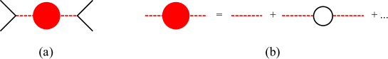
Figure 1: The scattering matrix for the process $\phi_{1}\phi_{2}\to\phi_{1}\phi_{2}$ (a) and the two-point function of the field $\Phi$ (b). Only one-loop bubbles are summed up. Solid (dashed) lines denote $\phi_{1,2}$ ($\Phi$) fields, respectively.

The residue of the propagator determines the wave function renormalization constant for the particle $\Phi$:

$$Z=\frac{1}{1-g_{0}^{2}\,G^{\prime}(M^{2})}=1+g^{2}\,G^{\prime}(M^{2}),$$ (15)

where $g^{2}=Z\,g_{0}^{2}$ is the renormalized coupling constant, and $G^{\prime}(M^{2})=\left.\frac{d}{ds}G(s)\right|_{s=M^{2}}$. In order to establish the relation of the quantity $Z$, defined by Eq. (15), with its non-relativistic counterpart, we perform the contour integration over $q^{0}$ of the loop integral in Eq. (11):

$$G(s)=\int\!\frac{d^{3}\vec{q}}{(2\pi)^{3}}\frac{1}{2\omega_{1}\omega_{2}}\frac{\omega_{1}+\omega_{2}}{s+\vec{P}^{2}-(\omega_{1}+\omega_{2})^{2}+i\epsilon},$$ (16)

where $\omega_{1}^{2}=(\vec{P}-\vec{q}\,)^{2}+m_{1}^{2}$ and $\omega_{2}^{2}=\vec{q}^{\,2}+m_{2}^{2}$. In the rest frame of the bound state, one has $\vec{P}=0$. Taking derivative with respect to $s$, and then taking the non-relativistic approximation which amounts to $\omega_{1}\simeq m_{1}+\vec{q}^{\,2}/(2m_{1})$ and $\omega_{2}\simeq m_{2}+\vec{q}^{\,2}/(2m_{2})$, we get

$$g^{2}\,G^{\prime}(M^{2})\simeq-\frac{g^{2}}{8m_{1}m_{2}M}\int\!\frac{d^{3}\vec{q}}{(2\pi)^{3}}\frac{1}{\left[E_{B}+\vec{q}^{\,2}/(2\mu)\right]^{2}},$$ (17)

where we have used $E_{B}=m_{1}+m_{2}-M$. Taking into account the difference between relativistic and non-relativistic normalizations, we finally arrive at the relation $g=\sqrt{2m_{1}}\sqrt{2m_{2}}\sqrt{2M}g_{\text{NR}}$, cf. with Eq. (5). Comparing now this relation with Eq. (3), one immediately sees that the wave function renormalization constant $Z$ is the same as its non-relativistic counterpart and thus the compositeness condition for an S-wave bound state can be written as

$$Z=1+g^{2}\,G^{\prime}(M^{2})\to 0.$$ (18)

One might treat the above argumentation with a grain of salt, since it is based on certain approximations. Namely, the amplitude is given as a sum of one-loop diagrams only. It is, however, clear that the result is valid beyond this approximation, if bound states close to an elastic threshold are considered. The justification is provided by the statement that such bound states can be consistently described within a non-relativistic effective field theory, which is perturbatively matched to the underlying relativistic theory (see, e.g., Ref. Gasser:2007zt for a review on the subject). Such an effective theory is equivalent to the non-relativistic quantum mechanics (the number of particles is conserved) and hence the compositeness can be rigorously defined along the lines discussed above. Finally, we would like to mention that the quantity $Z$, which is defined in Eq. (15), is ultraviolet finite, since the quantity $g$ is defined through the residue of the renormalized scattering amplitude.

III Compositeness from lattice data

As stated above, the wave function renormalization constant, $Z$, gives an overlap of the physical state with the elementary state and hence could be used as a parameter that describes the compositeness of a given state. Lattice calculations provide a model-independent way to determine $Z$ from the volume dependence of the spectrum Sekihara:2012xp ; Luscher:1985dn ; Beane:2003da ; Koma:2004wz ; Sasaki:2006jn ; Davoudi:2011md , or – as we propose in this paper – from the dependence on the twisting angle. In this section we set up a finite-volume formalism, which describes the dependence of the bound-state mass on the volume or twisting angle.

III.1 Finite volume formalism

We consider elastic scattering of particles with the masses $m_{1}$ and $m_{2}$ in the S-wave. Then, generally, a unitary partial-wave amplitude in infinite volume is given by

$$T(s)=\frac{1}{V^{-1}(s)-G(s)}=\frac{-8\pi\sqrt{s}}{k\cot\delta(k)-ik},$$ (19)

where $k^{2}=\frac{1}{4s}[s-(m_{1}+m_{2})^{2}][s-(m_{1}-m_{2})^{2}]$ is the relative momentum squared in the center of mass (c.m.) frame. Further, the function $V^{-1}(s)$ (“the inverse potential”) is a regular function in the vicinity of the threshold. The notation used here is reminiscent of that of unitarized Chiral Perturbation Theory, but Eq. (19) may in fact describe any elastic unitary amplitude, with the particular dynamics encoded in the function $V(s)$. The loop function $G(s)$ is given by Eqs. (11) and (16). This function contains a unitarity cut. Across this cut, we have ${\mbox{Im}\,}G(s)=-k/(8\pi\sqrt{s})$. Other (distant) cuts that may be also present are included in $V(s)$. The loop function $G(s)$ is divergent and has to be renormalized. Here we do the renormalization with a subtraction constant. As it will be seen below, the extension to the finite volume is independent of any regulator.

When the particles are put in a finite box of size $L$, their momenta become discretized due to boundary conditions. So, the continuum spectrum, which gives rise to the cut in the infinite volume, becomes a discrete set of two-particle levels. In order to obtain the spectrum in a finite volume, one should replace the momentum integrals by the sums over the discretized momenta in the expression of the scattering amplitude. Then, the “finite volume scattering amplitude” $\tilde{T}$ contains poles on the real axis that correspond to the discrete two-particle levels. It should be noted that the finite-volume effects in $V(s)$ are exponentially suppressed (see, e.g., luescher-torus ), so the the finite volume scattering amplitude can be obtained just by changing the loop function by its finite volume counterpart $\tilde{G}_{L}^{\vec{\theta}}(s)=G(s)+\Delta G_{L}^{\vec{\theta}}(s)$ Doring:2011vk , where

$$\Delta G_{L}^{\vec{\theta}}(s)=\lim_{\Lambda\to\infty}\left[\frac{1}{L^{3}}\sum_{|\vec{q}_{n}|<\Lambda}I(\vec{q}_{n})-\int_{|\vec{q}|<\Lambda}\frac{d^{3}\vec{q}}{(2\pi)^{3}}I(\vec{q}\,)\right]\,.$$ (20)

Here $I(\vec{q}\,)$ denotes the integrand in Eq. (16), and $\vec{q}_{n}$ the allowed momenta in a finite volume, whose value depends on the box size $L$ and the boundary conditions used. For the periodic boundary conditions we have $\vec{q}_{n}=\frac{2\pi}{L}\vec{n}$, $\vec{n}\in\mathbb{Z}^{3}$. In case of twisted boundary conditions, the momenta also depend on the twisting angle $\vec{\theta}$ according to $\vec{q}_{n}=\frac{2\pi}{L}\vec{n}+\frac{\vec{\theta}}{L},~{}0\leq\theta_{i}<2\pi$. Using the methods of Ref. Doring:2011vk , it can be shown that $\Delta G_{L}^{\vec{\theta}}$ can be related to the modified Lüscher function $Z_{00}^{\vec{\theta}}$, see Appendix A,

$$\Delta G_{L}^{\vec{\theta}}(s)=\frac{1}{8\pi\sqrt{s}}\left(ik-\frac{2}{\sqrt{\pi}L}Z_{00}^{\vec{\theta}}(1,\hat{k}^{2})\right)+\cdots,$$ (21)

where $\hat{k}=kL/(2\pi)$ and the dots stand for terms that are exponentially suppressed with the volume size $L$ Doring:2011vk .

In this paper, we are going to apply Lüscher formalism to study shallow bound states, where the finite-volume effects are exponentially suppressed. Since, for such states, the binding momentum $\kappa$ is presumed to be much smaller than the lightest mass in the system, the exponentially suppressed corrections emerging, e.g., from the potential $V(s)$ could be consistently neglected as compared to the corrections $\sim e^{-\kappa L}$ that arise from $Z_{00}^{\vec{\theta}}(1,\hat{k}^{2})$. Note however that, if masses of the constituents increase for a fixed binding energy, then the magnitude of the binding momentum also increases and, for the bound states of heavy mesons, may become comparable to the pion mass. In this case, further study of the problem is necessary. A recent example of such a study (albeit in the light quark sector) is given in Ref. Albaladejo . In the present paper this issue is not addressed.

Finally, note that the divergences arising at $\Lambda\to\infty$ in Eq. (20) cancel between the sum and the integral, so we can safely send the cutoff to infinity. Thus, $\Delta G_{L}^{\vec{\theta}}$ does not depend on any regulator. In Appendix A we show in detail, how $\Delta G_{L}^{\vec{\theta}}$ could be calculated below threshold for different types of boundary conditions.

III.2 Bound states in finite volume

Bound states show up in the scattering amplitude as poles on the real axis below threshold. Namely, if we have a bound state with the mass $M$ in the infinite volume, the scattering amplitude should have a pole at $s=M^{2}$, with the corresponding binding momentum $k_{B}\equiv i\kappa$, $\kappa>0$. From Eq. (19), it is clear that $M$ and $k_{B}$ satisfy the equation

$$\psi(k_{B}^{2})+\kappa=-8\pi M\Big{[}V^{-1}(M^{2})-G(M^{2})\Big{]}=0,$$ (22)

where $\psi(k^{2})$ is the analytic continuation of $k\cot\delta(k)$ for arbitrary complex values of $k^{2}$, which is needed since the bound state is located below threshold, $k_{B}^{2}<0$. On the other hand, the discrete levels in a finite volume are obtained as the poles of the finite-volume scattering amplitude $\tilde{T}$ and, in particular, the bound state pole gets shifted to $M_{L}$, with binding momentum $k_{L}\equiv i\kappa_{L}$, given by

$$\tilde{T}^{-1}(M_{L}^{2})=T^{-1}(M_{L}^{2})-\Delta G_{L}^{\vec{\theta}}(M_{L}^{2})=0\quad\Rightarrow\quad\psi(k_{L}^{2})+\kappa_{L}+8\pi M_{L}\Delta G_{L}^{\vec{\theta}}(M_{L}^{2})=0\,.$$ (23)

Note that, below threshold, both $T^{-1}$ and $\Delta G_{L}^{\vec{\theta}}$ are real, so the pole position is real. The discrete scattering levels above threshold are real as well (as they should be), since the imaginary part of $\Delta G_{L}^{\vec{\theta}}$ cancels exactly with that of $T^{-1}$.

Next, we relate the finite-volume pole position with the infinite-volume quantities as the bound state mass, $M$, and the coupling, $g^{2}$ (defined as the residue of the scattering amplitude at the pole $s=M^{2}$). To this end, we expand $\psi(k_{L}^{2})$ around the infinite-volume pole position, $k_{B}=i\kappa$,

$$\psi(k_{L}^{2})\simeq\psi(k_{B}^{2})-\psi^{\prime}(k_{B}^{2})(\kappa_{L}^{2}-\kappa^{2})=-\kappa-\psi^{\prime}(k_{B}^{2})(\kappa_{L}-\kappa)(\kappa_{L}+\kappa),$$ (24)

where the prime denotes a derivative respect to $k^{2}$. Then, evaluating the residue at $M^{2}$ in Eq. (19) we obtain

$$\psi^{\prime}(k_{B}^{2})=\frac{1}{2\kappa}-\frac{8\pi M}{g^{2}\frac{dk^{2}}{ds}},$$ (25)

where the derivative $dk^{2}/ds$ is to be evaluated at $s=M^{2}$. Finally, using Eqs. (23) and (24), we obtain for the pole position shift

$$\kappa_{L}-\kappa=\frac{1}{1-2\kappa\psi^{\prime}(k_{B}^{2})}\left[-8\pi M_{L}\Delta G_{L}^{\vec{\theta}}(M_{L}^{2})+\psi^{\prime}(k_{B}^{2})(\kappa_{L}-\kappa)^{2}\right]$$ (26)

This equation gives the bound state pole position, $\kappa_{L}$ (or, equivalently, $M_{L}=\sqrt{m_{1}^{2}-\kappa_{L}^{2}}+\sqrt{m_{2}^{2}-\kappa_{L}^{2}}$) as a function of the infinite-volume parameters $g^{2}$ and $\kappa$. It is worth noting that, within the approximation (24), the position of the bound state pole in a finite volume depends only on these two parameters. This approximation works remarkably well in all cases considered in this paper.

If the difference $\kappa_{L}-\kappa$ is small enough, Eq. (26) can be solved iteratively. For periodic boundary conditions, with the use of Eq. (47), it can be shown that the lowest-order iterative solution reads

$$\kappa_{L}=\kappa+\frac{6}{1-2\kappa\psi^{\prime}(k_{B}^{2})}\,\frac{1}{L}\,e^{-\kappa L}\,,$$ (27)

which coincides with the result given in Refs. Sasaki:2006jn ; Beane:2003da ; Sekihara:2012xp . However, it will be shown below that, for shallow bound states, where $\kappa$ is very small, one should take more than just the first term in the sum (47). Moreover, in some cases, the iterations converge very slowly, if at all. Therefore, in our opinion, it is safer to consider solving Eq. (26) numerically, without further approximations, in order to obtain the finite volume pole position $\kappa_{L}$. This is the way we proceed.

Using Eq. (26), it is possible to fit the infinite-volume parameters $M$ and $g^{2}$ from the bound state levels $\kappa_{L}$, obtained through lattice simulations at different $L$ or $\vec{\theta}$. This, in turn, allows one to determine the compositeness parameter from Eq. (18). However, in actual lattice simulations, the measured energy levels have some uncertainty, and the number of different volumes or different twisting angles might be not very large. Therefore, it is important to know in advance, at which accuracy should be the lattice measurements carried out, in order to render the extraction of the parameter $Z$ reliable. We address this question in some exactly solvable models with a given $V(s)$, producing “synthetic lattice data,” adding random errors and trying to extract back the infinite volume parameters $M,g^{2}$ and $Z$ from data.

IV Analysis with two models

IV.1 A toy model

The potential in this model is given by a “bare state pole”,

$$V_{\sf toy}(s)=\frac{g_{0}^{2}}{s-s_{0}},$$ (28)

which depends on two parameters: a bare pole position $s_{0}$ and a bare coupling constant $g_{0}$. By appropriately choosing the value of the bare parameters, we can reproduce a bound state with any given mass $M$ and coupling $g$.

If our model describes the interaction of two particles, where a bound state with the mass $M$ is present, the scattering partial wave amplitude (19) should have a pole at $s=M^{2}$,

$$M^{2}-s_{0}-g_{0}^{2}G(M^{2})=0.$$ (29)

The physical coupling of the bound state, $g$, is given by the residue of the scattering partial-wave amplitude at the bound state pole

$$g^{2}=\frac{g_{0}^{2}}{1-g_{0}^{2}G^{\prime}(M^{2})}=[1+g^{2}G^{\prime}(M^{2})]g_{0}^{2}=Zg_{0}^{2}\,.$$ (30)

One can use above equations to trade the bare parameters for the physical ones in the expression of the scattering amplitude and write the latter in terms of $M$ and $Z$:

$$T_{\sf toy}(s)=\frac{Z-1}{(s-M^{2})ZG^{\prime}(M^{2})+(1-Z)[G(s)-G(M^{2})]}.$$ (31)

Note that the above amplitude does not depend on the subtraction constant that renders $G(s)$ finite. This model can describe a bound state with any given value of the wave function renormalization constant.

Next, we study the finite volume effects in the bound-state mass. In the actual calculations, we take $m_{1}=m_{D}$, $m_{2}=m_{K}$ and choose the mass of the bound state to be $M=2340$ MeV. This is a shallow bound state at 20 MeV below threshold, which corresponds to a binding momentum $\kappa\simeq 133$ MeV. For the mainly molecular state we take $Z=0.1$, and $Z=0.9$ is chosen for the mainly elementary one. For each of these two states, we calculate their finite-volume mass $M_{L}$ as the subthreshold pole position in the finite-volume scattering amplitude.

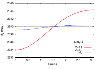
Figure 2: Bound state mass in the finite volume, $M_{L}$, as a function of $L$ for periodic boundary conditions (left) and as a function of the twisting angle for twisted boundary conditions (right). The solid/dashed lines correspond to $Z=0.1$ and $Z=0.9$, respectively. The dotted line stands for the infinite-volume mass $M$. In order to test the accuracy of the iterative solution, for the case of $Z=0.1$ we also plot (dot-dashed lines) the solutions of Eq. (26) with an approximate expression of $\Delta G_{L}^{\vec{\theta}}$ (only the first $n\equiv|\vec{n}|$ terms are retained in the expression (47) for $\Delta G_{L}^{\vec{\theta}}$).

In the left panel of Fig. 2, we show the mass of the two states with $Z=0.1$ and $Z=0.9$ as a function of $L$ for periodic boundary conditions. These are obtained from the solution of the exact equation (23). It is easy to see that the finite volume effects are much bigger in the case of the molecular state with $Z=0.1$ than in the case of an elementary state with $Z=0.9$. This was of course expected in advance, since small finite-volume effects point on a compact nature of the state in question. Here we also plot the solutions of Eq. (26), using the known values of $M$ and $g$, taken from the infinite volume model. In this way we can test the validity of the approximation in Eq. (24), used to derive Eq. (26) from Eq. (23), which basically states that all relevant dynamics is encoded only in the two parameters $M$ and $g$. As can be seen in Fig. 2, Eq. (26) is able to reproduce the synthetic lattice results very accurately. On the other hand, note that for shallow bound states the binding momentum $\kappa$ is small, so no wonder that the expansion in $\Delta G_{L}^{\vec{\theta}}$ converges rather slowly. Consequently, retaining only the leading-order term and constructing iterative solution, see Eq. (27), might not be sufficient in all cases.

In the right panel of the same figure we show the dependence of the bound-state mass on the twisting angle $\vec{\theta}=(\theta,\theta,\theta)$ for the fixed value of $Lm_{\pi}=3$. We see that, for such a choice of twisting, the size of the effect of twisting for a fixed $L$ is almost the double of the maximal effect caused by the variation of $L$ from the same value to infinity (periodic boundary conditions). Thus, using (partially) twisted boundary conditions to determine $Z$, besides being cheaper, could give more accurate results than a method based on the study of the volume-dependence of the energy level. Note also that, for the above choice of the twisting angle, the twisting effect is maximal. Other choices, e.g., $\vec{\theta}=(0,0,\theta)$ lead to a smaller effect.

IV.2 $DK$ scattering and the $D_{s0}^{*}(2317)$

Now we turn our attention to the realistic case of the hadronic bound state $D_{s0}^{*}(2317)$ in the $DK$ scattering channel with isospin $I=0$ and strangeness $S=1$. When isospin symmetry is exact, this state is stable under strong interactions, since it does not couple to the lighter hadronic channels (the observed decay $D_{s0}^{*}(2317)\to D_{s}\pi$ breaks isospin symmetry). Thus, the formalism above, tailored for stable bound states, does apply in this case. The case of quasi-bound states, which are coupled to inelastic channels, requires special treatment and is not addressed here.

A popular view on the $D_{s0}^{*}(2317)$ meson is that this state is dynamically generated as a pole through the S-wave interactions between the $D$-meson and the kaon in the isoscalar channel Kolomeitsev:2003ac ; Guo:2006fu ; Hofmann:2003je ; Gamermann:2006nm ; Guo:2009ct ; Liu:2012zya . We shall study this system, using the model used from Ref. Guo:2006fu , which is based on the leading-order heavy flavor chiral Lagrangian Burdman ; Wise:1992hn ; Yan:1992gz and unitarizes the amplitude Oller:1997ti ; Oller:1997ng ; Oller:1998hw ; Nieves:1998hp . Namely, the infinite-volume amplitude is obtained from Eq. (19) with the S-wave-projected potential

$$V(s)=\frac{1}{2}\int_{-1}^{1}dx\,\frac{u(s,x)-s}{2f_{\pi}^{2}}=\frac{1}{2f_{\pi}^{2}}\left[m_{D}^{2}+m_{K}^{2}+\frac{(m_{D}^{2}-m_{K}^{2})^{2}}{2s}-\frac{3s}{2}\right],$$ (32)

where $x=\cos\theta$ is the cosine of the scattering angle, $f_{\pi}\simeq 92.4$ MeV is the pion decay constant, and $s$ and $u$ are usual Mandelstam variables. We regularize the loop function with a subtraction constant $a(\mu)$, as done in Refs. Oller-Meissner ; Guo:2006fu . Its value at the scale $\mu=m_{D}$ is taken to be $a(m_{D})=-0.71$. With this value of the subtraction constant, we find a bound state pole, associated with the $D_{s0}^{*}(2317)$, at $M=2316.9~{}\mbox{MeV}$, and the coupling to $DK$, which is given by the residue of the pole,

$$g^{2}=\lim_{s\to M^{2}}(s-M^{2})T(s),$$ (33)

takes the value $g=10.7~{}\mbox{GeV}$. One can easily calculate the compositeness parameter of the bound state as well, using Eq. (18). The calculation yields $Z=0.29$. Hence, in this model, the $D_{s}^{*}(2317)$ is predominately a molecular state.

Next, we study this model in a finite volume and consider twisting of different quarks, from which the $D$ and $K$ mesons consist. The net effect is that these mesons get different momenta as a result of such twisting, so the expression for $G_{L}^{\vec{\theta}}$ changes. Note that this issue is important in view of the fact that partial twisting is allowed only for certain quarks (see Section V for more details).

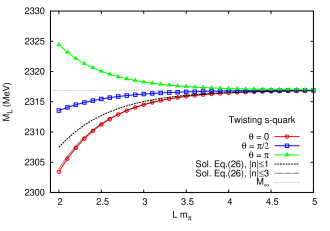
Figure 3: $L$-dependence of the $DK$ bound-state mass for different twisting angles. Left: twisted boundary conditions applied to the $u$-quark. Right: twisted boundary conditions applied to the $s$-quark. The dashed lines give the solution of Eq. (26), using the values for $M$ and $g$ from the infinite-volume model. In these solutions, approximate expression for $G_{L}^{\vec{\theta}}$ at $\vec{\theta}=0$ was used, that amounts to summing up exponentials only up to $|\vec{n}|\leq n_{max}$.

In Fig. 3, we display the volume dependence of the bound state mass for different twisting angles which are again chosen as $\vec{\theta}=(\theta,\theta,\theta)$. In the left panel, we plot the $L$-dependence for three different values of the twisting angle, when twisted boundary conditions are applied to the $u$-quark. In the right panel, twisted boundary conditions are applied to the $s$-quark. As we shall see later, in the latter case the use of partial twisting gives the same results as using fully twisted boundary conditions. The size of the finite volume effects, using twisted boundary conditions for the $c$-quark, is very small, so we do not discuss this case. In this model, we test again that the predictions obtained from Eq. (26), using the values of $M$ and $g$ from the infinite-volume model, reproduce very well the exact solution. Consequently, all relevant dynamics of the model near threshold is encoded in just two parameters $g$ and $M$. On the other hand, we see that retaining only the leading exponential in the expansion of $G_{L}^{\vec{\theta}}$ will have a large impact on the accuracy. Consequently, the first few terms should be retained. We see that the convergence is satisfactory: e.g., taking $n_{max}\geq 3$, where $n_{max}$ denotes the number of terms retained in the expansion, we see that the largest difference between the synthetic data and the prediction from Eq. (26) is less than 0.1 MeV.

Analyzing Fig. 3, we again come to the conclusion that the use of (partially) twisted boundary conditions can provide a better way to extract the compositeness parameter $Z$ from lattice results. This can already be seen by comparing the curves for $\theta=0$ and $\theta=\pi$. One namely observes that the size of the effect due to twisting at a fixed volume is almost twice as big as due to changing the volume for periodic boundary conditions.

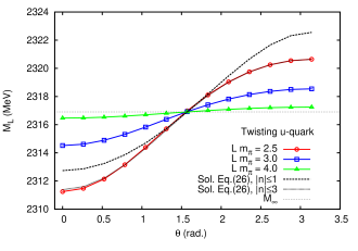
Figure 4: $\theta$ dependence of the $DK$ bound state mass for different lattice volumes. Left: twisted boundary conditions applied to the $u$-quark. Right: twisted boundary conditions applied to the $s$-quark. The dashed lines give the solution of Eq. (26), using the values for $M$ and $g$ from the infinite-volume model. In these solutions, approximate expression for $G_{L}^{\vec{\theta}}$ at $\vec{\theta}=0$ was used, that amounts to summing up exponentials only up to $|\vec{n}|\leq n_{max}$.

In Fig. 4, for three different volumes, we show the dependence of the bound-state mass on the twisting angle both for $u$- and $s$-quark twisting. On the other hand, taking the results of the $\theta$-dependence (like in Fig. 4) at a fixed volume for granted, one could fit the value of the infinite-volume mass and coupling constant to these data, using Eq. (26). After this, it is straightforward to obtain the value of $Z$. In fact, producing four synthetic lattice data points at a fixed $Lm_{\pi}=2.5$ and $\theta=0,\pi/3,2\pi/3,\pi$ (either for $u$- or $s$- quark twisting), we were able to obtain values for $M$ and $g$ that differ less than 1% from those calculated from the infinite volume model by fitting the solution to Eq. (26) (with $n_{max}=5$) to the synthetic data.

Real lattice simulations, however, produce results which carry uncertainties. Hence, the question arises, how big these errors could be in order to be still able to determine $Z$ with a desired accuracy. Since, as seen from the figures, the finite volume effects (for reasonable volume sizes, say, above $Lm_{\pi}=2.5$) are at most around 10 MeV, one expects that a relatively high accuracy will be needed in the measurement of the bound-state energy. In order to determine, how high this accuracy should actually be, we assign an uncertainty to the synthetic data that we generate from our model. In particular, using the von Neumann rejection method, from the “exact” data points we generate a new, “randomized” data set, where the central values of each data point are shifted randomly, following the Gaussian distribution centered at exact data values and with a standard deviation, given by the lattice data error. Repeating this process several times, we obtain several sets of synthetic lattice data with errors and central values shifted accordingly. We then fit each of the randomized data sets and obtain a corresponding value for $M$ and $g$ (and therefore, for $Z$), one for each set, ending up with as many values for the parameters, as many randomized data sets we have generated. We can obtain then the mean and standard deviation of the distributions for $M$, $g$ and $Z$. Thus, for a given data error, we can estimate the accuracy of the parameter extraction.

	4 lattice data points		8 lattice data points
$\Delta M_{L}$ (MeV)	$\;Lm_{\pi}=2.5\;$	$\;Lm_{\pi}=3.0\;$	$\;Lm_{\pi}=2.5\;$	$\;Lm_{\pi}=3.0\;$
2	0.21	0.47	0.17	0.36
1	0.11	0.23	0.08	0.19
0.5	0.05	0.12	0.04	0.09

Table 1: The accuracy of the extraction of the parameter $Z$ from the fits to the synthetic lattice data for different input error $\Delta M_{L}$. Four or eight data points and two different volumes $Lm_{\pi}=2.5$ and $Lm_{\pi}=3.0$ were used, see main text for details.

For the case of the $s$-quark twisting, we construct 5000 sets of randomized data at a fixed volume, for different input errors $\Delta M_{L}$ and different number of data points per set. Fitting the parameters to each set, we obtain the corresponding distributions of 5000 points for each parameter $M$, $g$ and $Z$. In table 1, we show the resulting standard deviations for $Z$, which give an idea of the expected accuracy in a fit to actual lattice data. The results for the case of the $u$-quark twisting are very similar. We see that, for $Lm_{\pi}=2.5$ where the finite volume effects are the largest, we need lattice errors smaller than 1 MeV in order to obtain an accuracy in $Z$ below 0.1. For larger volumes, the accuracy required in the input lattice data is even bigger. If we increase the number of lattice data points, we get slightly better results but, in general, the dependence on the increase of the size of the data set is very mild. For example, we need to use around 20 data points to achieve an accuracy of order 0.1 in $Z$, given an input error $\Delta M_{L}=2~{}\mbox{MeV}$ and volume $Lm_{\pi}=2.5$.

V Partially twisted boundary conditions in the $DK$ system

The partial twisting, unlike the full twisting, is more affordable in terms of computational cost in lattice simulations, because one does not need to generate new gauge configurations. Thus, it is very interesting to study whether it is possible to extract any physically relevant information from simulations using this kind of boundary conditions. Problems may arise when there are annihilation channels present, as is the case in the $DK$ scattering in the isoscalar channel, where light quarks may annihilate. An analysis of Lüscher approach with partial twisting for scattering problem in the presence of annihilation channels was recently addressed in Agadjanov:2013kja . Namely, a modified partially twisted Lüscher equation was derived for the $\pi\eta-K\bar{K}$ coupled channel scattering in the framework of non-relativistic EFT.

Index	Channel	Quark content
1	$|K_{\sf vv}D_{\sf vv}\rangle$	$-\frac{1}{\sqrt{2}}\,|u_{\sf v}\bar{s}_{\sf v}c_{\sf v}\bar{u}_{\sf v}+d_{\sf v}\bar{s}_{\sf v}c_{\sf v}\bar{d}_{\sf v}\rangle$
2	$|K_{\sf vs}D_{\sf vs}\rangle$	$-\frac{1}{\sqrt{2}}\,|u_{\sf s}\bar{s}_{\sf v}c_{\sf v}\bar{u}_{\sf s}+d_{\sf s}\bar{s}_{\sf v}c_{\sf v}\bar{d}_{\sf s}\rangle$
3	$|K_{\sf vg}D_{\sf vg}\rangle$	$-\frac{1}{\sqrt{2}}\,|u_{\sf g}\bar{s}_{\sf v}c_{\sf v}\bar{u}_{\sf g}+d_{\sf g}\bar{s}_{\sf v}c_{\sf v}\bar{d}_{\sf g}\rangle$

Table 2: Scattering channels for the case of $I=0$.

Here, we address the same problem in the context of the $DK$ scattering. The method is described in Ref. Agadjanov:2013kja , to which the reader is referred for further details. Consider first the scattering in the infinite volume. We start from building the channel space by tracking the quarks of different species following through the quark diagrams describing the $DK$ scattering. It is clear that, since only light quarks may annihilate, the possible final states contain valence, sea or ghost light quarks with equal masses, as given in table 2. Omitting channel indices, the resulting algebraic Lippmann-Schwinger equation couples 3 different channels

$$T=V+VG_{DK}T\,,$$ (34)

where $T$, $V$ and $G$ are given by $3\times 3$ matrices.

The free Green function is given by

$$G_{DK}(s)=G(s)~{}\mbox{diag}~{}(1,1,-1)$$ (35)

where $G(s)$ is defined in Eqs. (11) and (16), supplemented by the prescription that the integral is performed in dimensional regularization after expanding the integrand in powers of 3-momenta (see Refs. Agadjanov:2013kja ; cuspwe for details). The minus sign on the diagonal of the matrix $G$ arises due to fermionic nature of $D$ and $K$ mesons composed of valence and (commuting) ghost quarks.

The crucial point now is that there exist linear symmetry relations between various elements of $T$ due to equal valence, sea and ghost quark masses. Note that scattering matrix elements are given by residues of the 4-point Green functions $\Gamma_{ij}$ of the bilinear quark operators at the poles, corresponding to the external mesonic legs. Decomposing $\Gamma_{ij}$ into connected  $t_{c}$ and disconnected  $t_{d}$ pieces through Wick contractions (see Fig. 5) and noting that quark propagators are the same for all light quark species, we get

$$\Gamma_{11}=\Gamma_{22}=t_{c}-t_{d}\,,\quad\Gamma_{33}=-t_{c}-t_{d}\,,\quad\Gamma_{12}=\Gamma_{13}=\Gamma_{23}=\Gamma_{21}=\Gamma_{31}=\Gamma_{32}=-t_{d}\,,$$ (36)

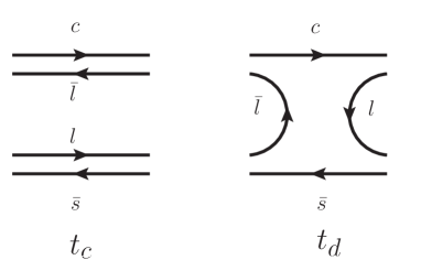
Figure 5: Connected ($t_{c}$) and disconnected ($t_{d}$) diagrams, emerging in $DK\to DK$ scattering amplitudes with various quark species; $l$=$u,d$.

Since in our case there are no neutral states and thus no mixing occurs, following the argumentation given in Ref. Agadjanov:2013kja , it is easy to show that $T$-matrix obeys the same symmetry relations as $\Gamma$

$$T_{11}=T_{22}=t,\quad T_{33}=-t+2y\,,\quad T_{12}=T_{13}=T_{23}=T_{21}=T_{31}=T_{32}=y\,.$$ (37)

Here $T_{11}=t$ corresponds to the physical elastic $DK$ scattering amplitude, i.e scattering in the sector with valence quarks only. Other diagonal entries are unphysical in the sense that they correspond to scattering of particles, composed of sea and ghost light quarks. Non-diagonal elements of $T$-matrix describe coupling between valence and sea/ghost sectors through disconnected diagrams. Furthermore, it is straightforward to check from Eq. (34) that the elements of potential matrix $V$ satisfy the same symmetry relations as $T$ and can be expressed in the following form

$$V=\left(\begin{array}[]{c c c }\tau&\upsilon&\upsilon\\ \upsilon&\tau&\upsilon\\ \upsilon&\upsilon&-\tau+2\upsilon\\ \end{array}\right)\,,$$ (41)

Let us now turn to the case of a finite volume and derive the Lüscher equation for a couple of particular choices of partially twisted boundary conditions. Note that the potential $V$ remains the same (up to exponentially suppressed in terms $L$ ), while in the loop functions the integration is substituted by summation over lattice momenta.

1. Twist the $s$/$c$-quark, leaving $u$ and $d$-quarks to obey periodic boundary condition. In this case, the matrix of the Green functions is $\text{diag}\left(\tilde{G}^{\vec{\theta}}_{L},\tilde{G}_{L}^{\vec{0}},-\tilde{G}_{L}^{\vec{0}}\right)$. The solution of the Lippmann-Schwinger equation in a finite volume for the physical amplitude $t$ is given by

   $$t=\frac{\tau}{1-\tau\tilde{G}_{L}^{\vec{\theta}}}\,,$$ (42)

   where $\tilde{G}_{L}^{\vec{\theta}}$ is the loop function $G(s)$ in a finite volume. We see that the finite-volume spectrum in case of the partial twisting is determined from the Lüscher equation

   $$1-\tau\tilde{G}_{L}^{\vec{\theta}}(s)=0,$$ (43)

   in the same way as in the full-twisting case. Thus, the results obtained by using of the partially twisted boundary conditions on the $c$- or $s$-quark are equivalent to those using full twisting.

2. Twist the valence $u$- and $d$-quarks simultaneously, leaving $s$- and $c$-quarks obey periodic boundary condition. In this case, the ghost light quarks also need to be twisted, and the matrix of the Green functions is $\text{diag}\left(\tilde{G}^{\vec{\theta}}_{L},\tilde{G}_{L}^{\vec{0}},-\tilde{G}_{L}^{\vec{\theta}}\right)$.

   The Lüscher equation determining the finite volume spectrum now takes the form

   $$\left[1-\tau\tilde{G}_{L}^{\vec{0}}(s)\right]\left[1-(\tau-\upsilon)\tilde{G}_{L}^{\vec{\theta}}(s)\right]^{2}=0\,.$$ (44)

   Vanishing of the first bracket on the r.h.s gives the Lüscher equation with no twisting. Note also that the quantity $\tau-\upsilon$ is in fact the connected part of the scattering potential for the isoscalar $DK$ system, which is identical to the $DK$ scattering potential in the isovector channel. Hence, vanishing of the second bracket is equivalent to the fully twisted Lüscher equation for the isovector $DK$ scattering .

VI Summary and conclusions

• Lattice QCD does not only determine the hadron spectrum. Under certain circumstances, it may provide information about the nature of hadrons, which renders lattice simulations extremely useful for the search and the identification of exotic states. Note that the lattice QCD possesses unique tools at its disposal (e.g., the study of the volume and quark mass dependence of the measured quantities), which are not available to experiment.

• In the present paper, we concentrate on the identification of hadronic molecules on the lattice. Experimentally, one may apply Weinberg’s compositeness condition to the near-threshold bound states, in order to distinguish the molecular states from the elementary ones. To this end, one may use the value of the wave function renormalization constant $Z$ which obeys the inequalities $0\leq Z\leq 1$. The vanishing value of the parameter $Z$ corresponds to the purely molecular state. In this paper we consider the lattice version of the Weinberg’s condition.

• It is known that the quantity $Z$ can be extracted from lattice data by studying the volume dependence of the measured energy spectrum. We have shown that the same result can be achieved by measuring the dependence of the spectrum on the twisting angle in case of twisted boundary conditions. Moreover, within the method proposed, the expected effect is approximately twice as large in magnitude and comes at a lower computational cost. Further, we have analyzed synthetic data to estimate the accuracy of the energy level measurement which is required for a reliable extraction of the value of $Z$ on the lattice.

• As an illustration of the method, we consider the $D_{s0}^{*}(2317)$ meson, which is a candidate of a $DK$ molecular state. It is proven that, despite the presence of the so-called annihilation diagrams, one may still use the partially twisted boundary conditions for the extraction of $Z$ from data if the charm or strange quark is twisted. The effects which emerge due to partial twisting, are suppressed at large volumes.

The authors thank M. Döring, L. Liu, U.-G. Meißner and S. Sasaki for interesting discussions. This work is partly supported by the EU Integrated Infrastructure Initiative HadronPhysics3 Project under Grant Agreement no. 283286. We also acknowledge the support by the DFG (CRC 16, “Subnuclear Structure of Matter”), by the DFG and NSFC (CRC 110, “Symmetries and the Emergence of Structure in QCD”), by the Shota Rustaveli National Science Foundation (Project DI/13/02), by the Bonn-Cologne Graduate School of Physics and Astronomy, by the NSFC (Grant No. 11165005), and by Volkswagenstiftung under contract No. 86260.

Appendix A Formulas for the function $\Delta G_{L}^{\vec{\theta}}$ below threshold

We compute the scattering amplitude in a finite volume by replacing the loop function $G$ by its finite volume counterpart $\tilde{G}_{L}^{\vec{\theta}}=G+\Delta G_{L}^{\vec{\theta}}$ and obtain synthetic data from the poles of the finite volume scattering amplitude. In particular, the pole below threshold gives the mass of the bound state in a finite volume.

For the case of a level below threshold, there exists a fairly simple way to calculate $\Delta G_{L}^{\vec{\theta}}$ defined by Eq. (20), so that the equation (26) for $\kappa_{L}$ can be easily solved. Here, we consider three different cases, one with periodic boundary conditions, and two with twisted boundary conditions. Depending on which quarks are twisted, the momenta of the mesons are modified accordingly.

A.1 Periodic boundary conditions

In the case of periodic boundary conditions, the meson momenta in a box are given by

$$\vec{q}_{n}=\frac{2\pi\vec{n}}{L},\qquad\vec{n}\in\mathbb{Z}^{3}.$$ (45)

We can evaluate the sum in Eq. (20), using the Poisson summation formula $\sum_{n}\delta(n-x)=\sum_{n}e^{2\pi inx}$. Transforming the sum into the integral gives

$$\frac{1}{L^{3}}\sum_{\vec{n}}I(\vec{q}_{n})=\frac{1}{L^{3}}\sum_{\vec{n}}\int d^{3}\vec{q}\,\,\delta^{(3)}(\vec{q}-\vec{q}_{n})I(\vec{q}\,)=\sum_{\vec{n}}\int\frac{d^{3}\vec{q}}{(2\pi)^{3}}\,\,e^{i\vec{q}\cdot\vec{n}L}I(\vec{q}\,).$$ (46)

Next, we note that the integrand $I(\vec{q}\,)$ can be approximated by $\frac{1}{2\sqrt{s}}\frac{1}{k^{2}-\vec{q}^{2}}$, since the difference is exponentially suppressed Doring:2011vk . Here, $k^{2}$ is the three-momentum squared of the particles in the center of mass (c.m.) frame. Then, for $k^{2}<0$, $\Delta G_{L}^{\vec{\theta}}$ reads

$$\Delta G_{L}^{\vec{0}}=\frac{1}{2\sqrt{s}}\sum_{\vec{n}\neq\vec{0}}\int\frac{d^{3}\vec{q}}{(2\pi)^{3}}\,\frac{e^{i\vec{q}\cdot\vec{n}L}}{k^{2}-\vec{q}^{2}}=-\frac{1}{8\pi\sqrt{s}L}\sum_{\vec{n}\neq\vec{0}}\frac{1}{|\vec{n}|}e^{-|\vec{n}|\sqrt{-k^{2}}L}.$$ (47)

The function $\Delta G_{L}^{\vec{0}}$ can be expressed in terms of the Lüscher zeta-function $Z_{00}(1,\hat{k}^{2})$, as follows Doring:2011vk :

$$\Delta G_{L}^{\vec{0}} = \frac{1}{8\pi\sqrt{s}}\left(-\sqrt{-k^{2}}-\frac{2}{\sqrt{\pi}L}Z_{00}(1,\hat{k}^{2})\right),$$ (48)

$$Z_{00}(1;\hat{k}^{2}) = \frac{1}{\sqrt{4\pi}}\,\sum_{{\vec{n}}\in\mathbb{Z}^{3}}\frac{1}{\vec{n}^{2}-\hat{k}^{2}}\,,$$ (49)

where $\hat{k}=kL/(2\pi)$.

A.2 Twisted boundary conditions: both momenta shifted

In the case of twisted boundary conditions, when the momenta of both particles are shifted but the particles still are in the c.m. frame, the allowed momenta in a box are:

$$\vec{q}_{n}=\frac{2\pi}{L}\vec{n}+\frac{\vec{\theta}}{L},\qquad\vec{n}\in\mathbb{Z}^{3}\,,$$ (50)

where $\vec{\theta}$ is the twisting angle. Now, acting in the same way, we can evaluate the sum in Eq. (20)

$$\frac{1}{L^{3}}\sum_{\vec{n}}I(\vec{q}_{n})=\frac{1}{L^{3}}\sum_{\vec{n}}\int d^{3}\vec{q}\,\,\delta^{(3)}(\vec{q}-\vec{q}_{n})I(\vec{q}\,)=\sum_{\vec{n}}\int\frac{d^{3}\vec{q}}{(2\pi)^{3}}\,\,e^{i\vec{\theta}\cdot\vec{n}}e^{i\vec{q}\cdot\vec{n}L}I(\vec{q}\,)$$ (51)

and $\Delta G_{L}^{\vec{\theta}}$ becomes

$$\Delta G_{L}^{\vec{\theta}}=-\frac{1}{8\pi\sqrt{s}L}\sum_{|\vec{n}|\neq 0}\frac{1}{|\vec{n}|}e^{i\vec{\theta}\cdot\vec{n}}e^{-|\vec{n}|\sqrt{-k^{2}}L}.$$ (52)

Again, we can express $\Delta G_{L}^{\vec{\theta}}$ in terms of the Lüscher zeta-function with twisted boundary conditions, $Z_{00}^{\vec{\theta}}(1,\hat{k}^{2})$, as follows,

$$\Delta G_{L}^{\vec{\theta}} = \frac{1}{8\pi\sqrt{s}}\left(-\sqrt{-k^{2}}-\frac{2}{\sqrt{\pi}L}Z_{00}^{\vec{\theta}}(1,\hat{k}^{2})\right),$$ (53)

$$Z_{00}^{\vec{\theta}}(1;\hat{k}^{2}) = \frac{1}{\sqrt{4\pi}}\,\sum_{{\vec{n}}\in\mathbb{Z}^{3}}\frac{1}{\bigl{(}\vec{n}+\vec{\theta}/2\pi\bigr{)}^{2}-\hat{k}^{2}}\,.$$ (54)

For the particular case of $\vec{\theta}=(\theta,\theta,\theta)$, the first few terms of the above expansion are given by

$$\Delta G_{L}^{(\theta,\theta,\theta)}(M)= -\frac{1}{8\pi ML}\Bigg{[}6\cos\,\theta\,e^{-\kappa L}+3\sqrt{2}(1+\cos 2\theta)e^{-\sqrt{2}\kappa L}$$

$$+\frac{2}{\sqrt{3}}(3\cos\theta+\cos 3\theta)e^{-\sqrt{3}\kappa L}+\cdots\Bigg{]}$$ (55)

with $\kappa=\sqrt{-k^{2}}$.

A.3 Twisted boundary conditions: only one momentum shifted

Finally, in the case of twisted boundary conditions, when only the momentum of one of the particles (say, particle 1) is shifted, the allowed momenta in a box are

$$\vec{q}_{1}=\frac{2\pi}{L}\vec{n}_{1}+\frac{\vec{\theta}}{L},\qquad\vec{q}_{2}=\frac{2\pi}{L}\vec{n}_{2},\qquad\vec{n}_{1},\vec{n}_{2}\in\mathbb{Z}^{3}\,.$$ (56)

The particles are not in the c.m. frame any more: the c.m. momentum is equal to $\vec{P}=\vec{\theta}/L$. Hence, we have to evaluate $\Delta G_{L}^{\vec{\theta}}$ in a moving frame with momentum $\vec{P}$,

$$\Delta G_{L}^{\vec{\theta}}= \frac{1}{L^{3}}\sum_{\vec{n}}I(\vec{q}_{n})-\int\frac{d^{3}\vec{q}}{(2\pi)^{3}}I(\vec{q}\,),\quad\quad I(\vec{q}\,)=\frac{1}{2\omega_{1}\omega_{2}}\frac{\omega_{1}+\omega_{2}}{P_{0}^{2}-(\omega_{1}+\omega_{2})^{2}},$$

$$\omega_{1}^{2}= (\vec{P}-\vec{q})^{2}+m_{1}^{2},\qquad\omega_{2}^{2}=\vec{q}^{2}+m_{2}^{2},\quad\quad\vec{q}_{n}=\frac{2\pi\vec{n}}{L},\qquad P^{2}=P_{0}^{2}-\vec{P}^{2}=s.$$ (57)

Again, we can approximate the integrand by Bernard:2012bi

$$I(\vec{q}\,)=-\frac{1}{2P_{0}}\frac{1}{(\vec{q}\,^{\prime})^{2}-(\vec{q}\,^{\prime}\cdot\vec{P})^{2}/P_{0}^{2}-\vec{k}^{2}}+\cdots,\qquad\vec{q}\,^{\prime}=\vec{q}-\mu\vec{P},$$ (58)

where $\mu=\frac{1}{2}\left(1-\frac{m_{1}^{2}-m_{2}^{2}}{s}\right)$, $\vec{k}$ is the momentum of the particles in the c.m. frame, and the dots denote exponentially suppressed terms. Using the Poisson summation formula, we arrive at

$$\Delta G_{L}^{\vec{\theta}}= -\frac{1}{2P_{0}}\sum_{|\vec{n}|\neq 0}e^{-i\mu\vec{P}\cdot\vec{n}L}\int\frac{d^{3}\vec{q}}{(2\pi)^{3}}\frac{e^{i\vec{q}\cdot\vec{n}L}}{\vec{q}^{2}-\vec{k}^{2}-\frac{(\vec{q}\cdot\vec{P})^{2}}{P_{0}^{2}}}$$ (59)

$$= -\frac{1}{8\pi\sqrt{s}L}\sum_{|\vec{n}|\neq 0}\frac{1}{|\hat{\gamma}\vec{n}|}e^{-i\mu\vec{\theta}\cdot\vec{n}}e^{-|\hat{\gamma}\vec{n}|\sqrt{-k^{2}}L},\quad\hat{\gamma}\vec{n}=\gamma\vec{n}_{\parallel}+\vec{n}_{\perp},$$ (60)

where $\vec{n}_{\parallel}$ and $\vec{n}_{\perp}$ are the components parallel and perpendicular to $\vec{P}$ of $\vec{n}$, and $\gamma=P_{0}/\sqrt{s}$ is the relativistic gamma-factor. Once again, we can relate $\Delta G_{L}^{\vec{\theta}}$ in this case with the Lüscher zeta function in the moving frame $Z_{00}^{\vec{d}}(1;(q^{*})^{2})$  Rummukainen , see also Refs. Schierholz ; Bernard:2012bi ; LiLiu :

$$\Delta G_{L}^{\vec{\theta}} = \frac{1}{8\pi\sqrt{s}}\left(-\sqrt{-k^{2}}-\frac{2}{\sqrt{\pi}L\gamma}Z_{00}^{\vec{d}}(1;\hat{k}^{2})\right),$$ (61)

$$Z_{00}^{\vec{d}}(1;\hat{k}^{2}) = \frac{1}{\sqrt{4\pi}}\,\sum_{{\vec{r}}\in P_{d}}\frac{1}{{\vec{r}}^{2}-\hat{k}^{2}}\,,$$

$$P_{d} = \{{\vec{r}}=\mathbb{R}^{3}~{}|~{}r_{\parallel}=\gamma^{-1}(n_{\parallel}-\mu|{\vec{d}}|),~{}{\vec{r}}_{\perp}={\vec{n}}_{\perp},~{}{\vec{n}}\in\mathbb{Z}^{3}\}\,,$$ (62)

where ${\vec{d}}={\vec{P}}L/2\pi=\vec{\theta}/2\pi$. For the case of $\vec{\theta}=(\theta,\theta,\theta)$, the first few terms in the above expansion are

$$\Delta G_{L}^{(\theta,\theta,\theta)}(M)= -\frac{1}{8\pi ML}\Bigg{[}\frac{6\sqrt{3}\cos(\mu\theta)}{\sqrt{\gamma^{2}+2}}e^{-\sqrt{\frac{\gamma^{2}+2}{3}}\,\kappa L}$$

$$+3\sqrt{2}e^{-\sqrt{2}\kappa L}+\frac{3\sqrt{6}\cos(2\mu\theta)}{\sqrt{2\gamma^{2}+1}}e^{-\sqrt{\frac{2}{3}(2\gamma^{2}+1)}\,\kappa L}+\cdots\Bigg{]}.$$ (63)

In the case of shallow bound states, the exponential factor $\kappa$ will be usually quite small, so in order to reproduce accurately the full function, one should take several terms in the expansion for $\Delta G_{L}^{\vec{\theta}}$ above.

References

- (1) R. L. Jaffe, Phys. Rev. D 15 (1977) 267.
- (2) D. Black et al, Phys. Rev. D 59 (1999) 074026 [arXiv:hep-ph/9808415].
- (3) N. N. Achasov and A. V. Kiselev, Phys. Rev. D 68 (2003) 014006 [arXiv:hep-ph/0212153].
- (4) J. R. Pelaez, Mod. Phys. Lett. A 19 (2004) 2879 [arXiv:hep-ph/0411107].
- (5) J. D. Weinstein and N. Isgur, Phys. Rev. Lett. 48 (1982) 659.
- (6) J. A. Oller, E. Oset and J. R. Pelaez, Phys. Rev. Lett. 80 (1998) 3452 [hep-ph/9803242].
- (7) J. A. Oller, E. Oset and J. R. Pelaez, Phys. Rev. D 59 (1999) 074001 [Erratum-ibid. D 60 (1999) 099906] [Erratum-ibid. D 75 (2007) 099903] [hep-ph/9804209].
- (8) J. A. Oller and E. Oset, Phys. Rev. D 60 (1999) 074023 [arXiv:hep-ph/9809337];
- (9) G. Janssen, B. C. Pearce, K. Holinde and J. Speth, Phys. Rev. D 52 (1995) 2690 [arXiv:nucl-th/9411021].
- (10) Z. -H. Guo and J. A. Oller, Phys. Rev. D 84 (2011) 034005 [arXiv:1104.2849 [hep-ph]].
- (11) S. Peris, M. Perrottet and E. de Rafael, JHEP 9805 (1998) 011 [arXiv:hep-ph/9805442]; V. Elias, A. H. Fariborz, F. Shi and T. G. Steele, Nucl. Phys. A 633 (1998) 279 [arXiv:hep-ph/9801415].
- (12) D. Morgan, Nucl. Phys. A 543 (1992) 632.
- (13) N. A. Törnqvist, Phys. Rev. D 51 (1995) 5312 [arXiv:hep-ph/9403234].
- (14) S. Weinberg, Phys. Rev. 137 (1965) B672.
- (15) D. Morgan and M. R. Pennington, Phys. Lett. B 258 (1991) 444 [Erratum-ibid. B 269 (1991) 477]; Phys. Rev. D 48 (1993) 1185.
- (16) V. Baru, J. Haidenbauer, C. Hanhart, Yu. Kalashnikova and A. E. Kudryavtsev, Phys. Lett. B 586 (2004) 53 [arXiv:hep-ph/0308129].
- (17) V. Baru, J. Haidenbauer, C. Hanhart, A. E. Kudryavtsev and U.-G. Meißner, Eur. Phys. J. A 23 (2005) 523 [arXiv:nucl-th/0410099].
- (18) C. Hanhart, Eur. Phys. J. A 31 (2007) 543 [arXiv:hep-ph/0609136].
- (19) C. Hanhart, Eur. Phys. J. A 35 (2008) 271 [arXiv:0711.0578 [hep-ph]].
- (20) T. Hyodo, D. Jido and A. Hosaka, Phys. Rev. C 85 (2012) 015201 [arXiv:1108.5524 [nucl-th]].
- (21) T. Hyodo, Int. J. Mod. Phys. A 28 (2013) 1330045 [arXiv:1310.1176 [hep-ph]].
- (22) J. Nebreda, J. R. Pelaez and G. Rios, Phys. Rev. D 84 (2011) 074003 [arXiv:1107.4200 [hep-ph]].
- (23) J. R. Pelaez and G. Rios, Phys. Rev. Lett. 97 (2006) 242002 [hep-ph/0610397].
- (24) C. Hanhart, J. R. Pelaez and G. Rios, Phys. Rev. Lett. 100 (2008) 152001 [arXiv:0801.2871 [hep-ph]].
- (25) J. R. Pelaez and G. Rios, Phys. Rev. D 82 (2010) 114002 [arXiv:1010.6008 [hep-ph]].
- (26) V. Bernard, M. Lage, U.-G. Meißner and A. Rusetsky, JHEP 1101 (2011) 019 [arXiv:1010.6018 [hep-lat]].
- (27) M. Albaladejo and J. A. Oller, Phys. Rev. D 86 (2012) 034003 [arXiv:1205.6606 [hep-ph]].
- (28) F. Okiharu et al., arXiv:hep-ph/0507187; H. Suganuma, K. Tsumura, N. Ishii and F. Okiharu, PoS LAT2005 (2006) 070 [arXiv:hep-lat/0509121]; Prog. Theor. Phys. Suppl. 168 (2007) 168 [arXiv:0707.3309 [hep-lat]].
- (29) A. Martinez Torres, L. R. Dai, C. Koren, D. Jido and E. Oset, Phys. Rev. D 85 (2012) 014027 [arXiv:1109.0396 [hep-lat]].
- (30) T. Sekihara and T. Hyodo, Phys. Rev. C 87 (2013) 045202 [arXiv:1209.0577 [nucl-th]].
- (31) S. Ozaki and S. Sasaki, Phys. Rev. D 87 (2013) 014506 [arXiv:1211.5512 [hep-lat]].
- (32) M. Albaladejo, C. Hidalgo-Duque, J. Nieves and E. Oset, Phys. Rev. D 88 (2013) 014510 [arXiv:1304.1439 [hep-lat]].
- (33) B. Aubert et al. [BaBar Collaboration], Phys. Rev. Lett. 90 (2003) 242001 [hep-ex/0304021]; D. Besson et al. [CLEO Collaboration], Phys. Rev. D 68 (2003) 032002 [Erratum-ibid. D 75 (2007) 119908] [hep-ex/0305100].
- (34) S.-L. Zhu, Int. J. Mod. Phys. E 17 (2008) 283 [hep-ph/0703225].
- (35) M. Cleven, F. K.-Guo, C. Hanhart and U.-G. Meißner, Eur. Phys. J. A 47 (2011) 19 [arXiv:1009.3804 [hep-ph]].
- (36) L. Liu, K. Orginos, F.-K. Guo, C. Hanhart and U.-G. Meißner, Phys. Rev. D 87 (2013) 014508 [arXiv:1208.4535 [hep-lat]].
- (37) G. Moir, M. Peardon, S. M. Ryan, C. E. Thomas and L. Liu, arXiv:1312.1361 [hep-lat].
- (38) D. Mohler, C. B. Lang, L. Leskovec, S. Prelovsek and R. M. Woloshyn, Phys. Rev. Lett. 111 (2013) 22, 222001 [arXiv:1308.3175 [hep-lat]]; C. B. Lang, L. Leskovec, D. Mohler, S. Prelovsek and R. M. Woloshyn, Phys. Rev. D 90 (2014) 034510 [arXiv:1403.8103 [hep-lat]].
- (39) D. Agadjanov, U.-G. Meißner and A. Rusetsky, JHEP 1401 (2014) 103 [arXiv:1310.7183 [hep-lat]].
- (40) J. C. Howard and B. Jouvet, Nuovo Cim. 18 (1960) 466.
- (41) M. T. Vaughan, R.Aaron and R. D. Amado, Phys. Rev. 124 (1961) 1258.
- (42) A. Salam, Nuovo Cim. 25 (1962) 224.
- (43) S. Weinberg, Phys. Rev. 130 (1963) 776.
- (44) S. Weinberg, Lectures on Quantum Mechanics, Cambridge University Press, 2012.
- (45) F.-K. Guo, C. Hanhart, U.-G. Meißner, Q. Wang and Q. Zhao, Phys. Lett. B 725 (2013) 127 [arXiv:1306.3096 [hep-ph]].
- (46) J. Gasser, V. E. Lyubovitskij and A. Rusetsky, Phys. Rept. 456 (2008) 167 [arXiv:0711.3522 [hep-ph]].
- (47) M. Lüscher, Commun. Math. Phys. 104 (1986) 177.
- (48) S. R. Beane, P. F. Bedaque, A. Parreno and M. J. Savage, Phys. Lett. B 585 (2004) 106 [hep-lat/0312004].
- (49) Y. Koma and M. Koma, Nucl. Phys. B 713 (2005) 575 [hep-lat/0406034].
- (50) S. Sasaki and T. Yamazaki, Phys. Rev. D 74 (2006) 114507 [hep-lat/0610081].
- (51) Z. Davoudi and M. J. Savage, Phys. Rev. D 84 (2011) 114502 [arXiv:1108.5371 [hep-lat]].
- (52) M. Lüscher, Nucl. Phys. B 354 (1991) 531.
- (53) M. Döring, U.-G. Meißner, E. Oset and A. Rusetsky, Eur. Phys. J. A 47 (2011) 139 [arXiv:1107.3988 [hep-lat]].
- (54) M. Albaladejo, G. Rios, J. A. Oller and L. Roca, arXiv:1307.5169 [hep-lat].
- (55) E. E. Kolomeitsev and M. F. M. Lutz, Phys. Lett. B 582 (2004) 39 [hep-ph/0307133].
- (56) F.-K. Guo, P.-N. Shen, H.-C. Chiang, R.-G. Ping and B.-S. Zou, Phys. Lett. B 641 (2006) 278 [hep-ph/0603072].
- (57) J. Hofmann and M. F. M. Lutz, Nucl. Phys. A 733 (2004) 142 [hep-ph/0308263].
- (58) D. Gamermann, E. Oset, D. Strottman and M. J. Vicente Vacas, Phys. Rev. D 76 (2007) 074016 [hep-ph/0612179].
- (59) F.-K. Guo, C. Hanhart and U.-G. Meißner, Eur. Phys. J. A 40 (2009) 171 [arXiv:0901.1597 [hep-ph]].
- (60) G. Burdman and J. F. Donoghue, Phys. Lett. B 280 (1992) 287.
- (61) M. B. Wise, Phys. Rev. D 45 (1992) 2188.
- (62) T. -M. Yan, H. -Y. Cheng, C. -Y. Cheung, G. -L. Lin, Y. C. Lin and H. -L. Yu, Phys. Rev. D 46 (1992) 1148 [Erratum-ibid. D 55 (1997) 5851].
- (63) J. A. Oller and E. Oset, Nucl. Phys. A 620 (1997) 438 [Erratum-ibid. A 652 (1999) 407] [hep-ph/9702314].
- (64) J. Nieves and E. Ruiz Arriola, Phys. Lett. B 455 (1999) 30 [nucl-th/9807035].
- (65) J. A. Oller and U.-G. Meißner, Phys. Lett. B 500 (2001) 263 [hep-ph/0011146].
- (66) J. Gasser, B. Kubis and A. Rusetsky, Nucl. Phys. B 850 (2011) 96 [arXiv:1103.4273 [hep-ph]].
- (67) V. Bernard, D. Hoja, U.-G. Meißner and A. Rusetsky, JHEP 1209 (2012) 023 [arXiv:1205.4642 [hep-lat]].
- (68) K. Rummukainen and S. A. Gottlieb, Nucl. Phys. B 450 (1995) 397 [hep-lat/9503028].
- (69) M. Göckeler, R. Horsley, M. Lage, U.-G. Meißner, P. E. L. Rakow, A. Rusetsky, G. Schierholz and J. M. Zanotti, Phys. Rev. D 86 (2012) 094513 [arXiv:1206.4141 [hep-lat]].
- (70) N. Li and C. Liu, Phys. Rev. D 87 (2013) 014502 [arXiv:1209.2201 [hep-lat]].