On the pseudospectrum of the harmonic oscillator with imaginary cubic potential
Abstract
We study the Schrödinger operator with a potential given by the sum of the potentials for harmonic oscillator and imaginary cubic oscillator and we focus on its pseudospectral properties. A summary of known results about the operator and its spectrum is provided and the importance of examining its pseudospectrum as well is emphasized. This is achieved by employing scaling techniques and treating the operator using semiclassical methods. The existence of pseudoeigenvalues very far from the spectrum is proven, and as a consequence, the spectrum of the operator is unstable with respect to small perturbations and the operator cannot be similar to a self-adjoint operator via a bounded and boundedly invertible transformation. It is shown that its eigenfunctions form a complete set in the Hilbert space of square-integrable functions; however, they do not form a Schauder basis.
Key words: pseudospectrum, harmonic oscillator, imaginary qubic potential, -symmetry, semiclassical method
Mathematics Subject Classification (2010): 35J05, 35P15, 47B44
1 Introduction
One of the first observations of purely real spectrum in a non-self-adjoint Schrödinger operator occured in [6] by Caliceti et al. The authors studied the class of operators on for a general complex and noticed that the spectrum is real provided and is sufficiently small. This property was later attributed to the -symmetry of the considered operator. The so-called -symmetric quantum mechanics originated with the numerical observation of a purely real spectrum of an imaginary cubic oscillator Hamiltonian [5] and rapidly developed thenceforth. See e.g. [4, 21] and references therein for a survey of papers in this area. The -symmetry property of an operator should be understood in this paper as the invariance of with respect to the space inversion and the time reversal on the Hilbert space , i.e.
| (1.1) |
in the operator sense, where stands for spatial reflection and stands for time reversal in quantum mechanics. Such operator possesses a relevant physical interpretation as an observable in quantum mechanics provided it is similar to a self-adjoint operator
| (1.2) |
where is a bounded and boundedly invertible operator. Then it is ensured that the spectra of and are identical and that the corresponding families of eigenfunctions share essential basis properties [19]. The similarity to a self-adjoint operator is in fact equivalent to the quasi-self-adjointness of ,
| (1.3) |
where the operator is positive, bounded and boundedly invertible [17, 23]. It is often called a metric, since the operator can be seen as self-adjoint in the space with the modified scalar product . The equivalence can be easily seen from the decomposition of a positive operator [18, Prop. 1.8].
In recent years it has been shown that the spectrum is not necessarily the best notion to describe properties of a non-self-adjoint operator and the use of -pseudospectrum, denoted here and defined as
| (1.4) |
was suggested instead [7, 11, 16, 18, 19, 25, 27]. In [25] authors studied the operator and derived completeness of its eigenfunctions, found the bounded metric operator and proved that it can not have a bounded inverse. These results were further supplemented in [19] where the existence of points in the pseudospectrum far from the spectrum was established. This paper aims to apply the methods used in these papers to the operator , whose several properties were investigated e.g. in [6, 10, 14, 20]. Our aim is to establish results which can be directly extended to the more general case , . We choose to study the case to show its relation to the famous imaginary cubic oscillator.
Let us consider the Hilbert space and define the operator acting on its maximal domain:
| (1.5) | ||||
It was shown in [6] that coincides with and that is closed. Furthermore, it is an operator with compact resolvent and therefore its spectrum is discrete (i.e. consists of isolated eigenvalues of finite algebraic multiplicity). The reality and the simplicity of the eigenvalues was established in [24]. Using the approach of [13, Sec. VII.2] shows that coincides with the closure of (1.5) defined on smooth functions with compact support and that it is an m-accretive operator. Recall that this means that is closed and that and for . In this paper we contribute to these results with showing the non-triviality of the pseudospectrum of and demonstrating its several consequences. The main results are summarised in the following theorem.
Theorem 1.1.
Let be the operator defined in (1.5). Then:
-
1.
The eigenfunctions of form a complete set in .
-
2.
The eigenfunctions of do not form a (Schauder) basis in .
-
3.
For any there exist constants such that for all small,
(1.6) -
4.
is not similar to a self-adjoint operator via bounded and boundedly invertible transformation
-
5.
is not quasi-self-adjoint with a bounded and boundedly invertible metric.
-
6.
is not a generator of a bounded semigroup.
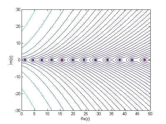
We can see that for any the pseudospectrum contains complex points with positive real part, non-negative imaginary part and large magnitude. This result is in particular important in view of the characterisation of pseudospectrum (2.3) – it implies the existence of pseudomodes very far from the spectrum. This non-trivial behaviour of the pseudospectrum was without details announced in [25]. A numerical computation of several of the pseudospectral lines of can be seen in Figure 1. As a consequence of the last point in Theorem 1.1, the time-dependent Schrödinger equation with does not admit a bounded time-evolution. For more details about establishing a time-evolution of an unbounded non-self-adjoint operator we refer to recent papers [1, 2] and to references therein.
This paper is organised as follows. In Section 2 we formulate some properties of pseudospectrum to emphasize its importance in the study of non-self-adjoint operators. In Section 3 we develop a semiclassical technique applicable in the study of pseudospectrum of the present model. The proof of the main theorem of the paper about pseudospectrum and eigenfunctions of can be found in Section 4. The Section 5 is devoted to a discussion of the results and of their consequences.
2 General aspects of the pseudospectrum
The definition of the pseudospectrum and some of its most prominent properties are presented in this section. The focus is on properties related to this paper, which were already highlighted in [19], where the authors dealt with similar problems. The presented list is far from complete and we refer to the monographs [9, 27] for more details on this subject.
Let be a closed densely defined operator on a complex Hilbert space . Its spectrum is defined as the set of complex points for which the operator does not exist or is not bounded on . The complement of this set in is called the resolvent set of . It is a well known fact that the spectrum of a bounded linear operator is contained in the closure of its numerical range . Moreover, this holds for closed unbounded operators as well, provided the exterior of the numerical range in is a connected set and has a non-empty intersection with the resolvent set of . The -pseudospectrum (or simply pseudospectrum) of is defined as
| (2.1) |
with the convention that for . In other words, for every from the definition and from the inequality we can easily see that also an -neighbourhood of the spectrum is contained in the pseudospectrum. Similarly as in the previous case, if the exterior of the numerical range in is a connected set and has a non-empty intersection with the resolvent set of , the pseudospectrum is in turn contained in the -neighbourhood of the numerical range, i.e. altogether we have
| (2.2) |
Perhaps the most striking property of pseudospectrum is provided by result sometimes known as Roch-Silberman theorem [22]. The -pseudospectrum of may be expressed via the spectra of all perturbations of of size less than :
| (2.3) |
This result is especially important in the study of non-self-adjoint operators. For operators with highly non-trivial pseudospectrum (i.e. not contained in some bounded neighbourhood of the spectrum) it reveals their spectral instability with respect to small perturbations. It also shows a difficulty in the numerical study of operators with wild pseudospectra – small rounding errors can lead to computing (false) eigenvalues, which are in fact very far from the true spectrum.
The pseudospectrum can also by characterised as the set of all points of the spectrum and of all pseudoeigenvalues (or approximate eigenvalues), i.e.
| (2.4) |
Any satisfying the inequality in (2.4) is called a pseudoeigenvector (or pseudomode). It can be easily seen that pseudoeigenvalues can be turned into eigenvalues by a small perturbation. If were to represent a physical observable and its perturbation, this fact would cause some highly unintuitive behaviour of its energies.
3 Semiclassical techniques
The use of semiclassical techniques in the study of non-self-adjoint operators was first suggested in [7], and the idea was further developed e.g. in [11, 28]. Let be an operator acting in of the form
| (3.1) |
Here are analytic potentials in for all small enough which take the form , where locally uniformly as . This operator should be understood as some closed extension of an operator originally defined on . The following theorem is an analogue of [7, Thm. 1] for a potential depending on . We postpone its proof into the following section.
Theorem 3.1.
Let be defined as above and let be from the set
| (3.2) |
where the dash denotes standard differentiation with respect to in . Then there exists some , some , and an -dependent family of functions with the property that, for all ,
| (3.3) |
The function is called the symbol associated with . Note that relation (2.4) gives us that for all . Here can get arbitrarily close to , provided is sufficiently small. The closure of is usually called the semiclassical pseudospectrum [11]. Application of Theorem 3.1 to non-semiclassical operators is sometimes possible by using scaling techniques and sending the spectral parameter to infinity. This is based on a more general principle that the semiclassical limit is equivalent to the high-energy limit after a change of variables.
Proof.
The proof is inspired by the proof of [19, Thm. 1]. We are interested in the case when is very close to , during the course of the proof we are not going to stress every occasion when this plays a role. We can assume to be “sufficiently small” when necessary. Let and assume . Let us notice that is dependent on from definition so changing in the course of our proof would mean changing as well. This problem can be overcome by fixing and introduce a dependence of and on in such a way that , where and as . The existence of these functions is ensured by the implicit function theorem. Since we only need to find one function for which (3.3) holds, the main idea is that the sought pseudomode will arise from JWKB approximation of the solution to which takes the form
| (3.4) |
where are functions analytic near . We follow here the procedure of constructing appropriate functions and as shown e.g. in [12, Chap. 2]. The function should satisfy the eikonal equation
| (3.5) |
where is the symbol associated with . (The dash denotes differentiation with respect to .) From this equation immediately follows that . The sign is determined by the condition applied in the point and remains the same for all . Therefore the sign of should be opposite of the sign of . Therefore we get
| (3.6) |
We need to check whether is analytic near for small. From the assumption we know that , so there exists such that for . Then for every , where and as , we get
| (3.7) |
for going to . Without loss of generality it is possible to assume , therefore can be fixed so that for some . Taking small, gets close to uniformly and , thus and consequently the square root in the definition of is well-defined. The case is proven in the same manner. After a translation we can assume further on .
The equality
| (3.8) |
can be verified with a direct computation. If we set so that they satisfy the transport equations
| (3.9) | ||||
for , we get that
| (3.10) |
We can also set and for and all . The equations (3.9) can be then solved using the method of integrating factor as
| (3.11) | ||||
These functions are well defined and analytic near thanks to analyticity of . We now proceed with estimates of the functions . Note that since the potentials are analytic, we can naturally extend them into the complex plane in the neighbourhood of and thus the same can be applied on and all . Our goal is to arrive to the estimate
| (3.12) |
for and in some neighbourhood of the origin. Then we will be able to define the -dependent function
| (3.13) |
which is uniformly bounded analytic function on the set where (3.12) holds due to the absolute summability of the sum
| (3.14) |
In the following we will derive the estimate (3.12) for extended to the complex plane (further denoted as ). With the natural choice of the norm
| (3.15) |
where is an open ball in the complex plane with center at and diameter , we easily see that the estimate obtained for will remained valid for in some neighbourhood of the origin. We fix such that, on , is analytic, is bounded from below and above and for some . We also employ Cauchy’s estimate for the second derivative of an analytic bounded function defined on :
| (3.16) |
With the use of the formula (3.11) we obtain
| (3.17) | ||||
for . We iterate these estimates on balls of radius , . Then we have for
| (3.18) |
Then it follows for that
| (3.19) |
Subsequently using these estimates for and taking a supremum we obtain
| (3.20) |
We see from (3.11) and our choice of that and from the uniform estimate of from below that , where the positive constants and does not depend on . The desired estimate (3.12) then follows with the constant
| (3.21) |
We are now able to define the desired pseudomode as
| (3.22) |
where is the function defined in (3.13) and such that it is identically equal to in some neighbourhood of and its support lies inside the interval . We divide the calculation of the norm in (3.3) as follows:
| (3.23) |
First we focus on the first summand. Since , is real and holds, we have
| (3.24) |
for all . Since on , we can use (3.10) to estimate
| (3.25) |
where . (Here denotes the floor function.) Using the estimate from (3.12) and the Cauchy’s estimate (3.16) we obtain for all that for independent of . From this the estimate
| (3.26) |
follows. To estimate the second summand in (3.23) we directly calculate
| (3.27) |
Using (3.14) we have uniform bounds on and thus on after the use of the Cauchy’s estimate (3.16), is bounded by the choice of , and are identically equal to on and is again bounded by (3.24) we see that (3.27) is in fact equal to on the neighborhood of , where is constant.
To complete the proof, it remains to show that defined in (3.22) is not exponentially small. Since we have established the estimate (3.12) for and , we have the estimate
| (3.28) |
for , where is sufficiently small. We can take very small and fixed, so because is close to and is close to for small, we obtain
| (3.29) |
∎
4 The proof of Theorem 1.1
For the sake of clarity we choose to divide the proof into several lemmas.
Lemma 4.1.
The eigenfunctions of form a complete set in .
Proof.
Let us first briefly recall that completeness of means that the span of is dense in . Since is m-accretive, its resolvent is m-accretive as well. It is also a Hilbert-Schmidt operator [6] and the application of [3, Thm. 1.3] yields that it is trace class as well. The completeness of its eigenfunctions follows from [15, Thm. X.3.1]. The completeness of eigenfunctions of then follows from the application of the spectral mapping theorem [13, Thm. IX.2.3]. ∎
Lemma 4.2.
For any there exist constants such that for all small,
| (4.1) |
Proof.
Using the unitary transformation
| (4.2) |
the semiclassical analogue of is introduced:
| (4.3) |
where
| (4.4) |
and . For the set from Theorem 3.1 holds . This theorem gives us that for any , and sufficiently small
| (4.5) |
holds. Let us define the set
| (4.6) |
for any . Then we see from the inequality (4.5) that for every and every sufficiently large, in particular such that the inequality holds. We may then identify the points of in absolute value with , i.e. . After we take logarithm of the lastly mentioned inequality and neglect the term which is small compared to for large, the statement of the theorem follows after expressing the inequality in terms of . ∎
Lemma 4.3.
The eigenfunctions of do not form a (Schauder) basis in .
Proof.
Let us first recall that a Schauder basis is a set such that for every element can be uniquely expressed as , where for . From the inequality (4.5) we can clearly see that the norm of the resolvent shoots up exponentially fast for large. Therefore the eigenfunctions of cannot be tame by [8, Thm. 3]. Specifically, if we arrange the eigenvalues of in increasing order, the norm of spectral projection corresponding to cannot satisfy
| (4.7) |
for some and all . Therefore cannot form a basis. ∎
Lemma 4.4.
is not a generator of a bounded semigroup.
Proof.
As in the previous proof, since the norm of resolvents grows exponentially for large, the claim follows from [9, Thm. 8.2.1]. ∎
The following result is a direct consequence of several propositions about operators with non-trivial pseudospectra from [19] which apply to as well. We summarise them and provide a compact proof.
Lemma 4.5.
is not similar to a self-adjoint operator via bounded and boundedly invertible transformation and is not quasi-self-adjoint with a bounded and boundedly invertible metric.
Proof.
If were similar to a self-adjoint operator as in (1.2), its pseudospectrum would have to satisfy
| (4.8) |
where . However, since the pseudospectrum of is just the -neighbourhood of its spectrum, it cannot contain arbitrarily large points as -pseudospectrum of does. The claim about the quasi-self-adjointness (1.3) follows from the already established equivalence from the decomposition . ∎
5 Summary
The harmonic oscillator coupled with an imaginary cubic oscillator potential was the main subject of interest of the present paper and we aimed to provide a detailed study of its basis and pseudospectral properties. The pseudospectrum of exhibits wild properties and contains points very far from the spectrum, which can be turned into true eigenvalues by a small perturbation of the operator. As a consequence, the eigenfunctions of do not form a Schauder basis, although they form a dense set in . The semigroup associated with the time-dependent Schödinger equation then does not have an expansion in the basis of eigenfunctions and does not admit a bounded time-evolution. The non-trivial pseudospectrum also implies that the considered operator does not have any bounded and boundedly invertible metric and thus it cannot be faithfully represented by any self-adjoint operator in the framework of standard quantum mechanics. In conclusion let us note that all results of this paper can be directly generalised to potentials of the type , since all previous cited results apply to this more general case as well.
Acknowledgements
The research was supported by the Czech Science Foundation within the project 14-06818S and by Grant Agency of the Czech Technical University in Prague, grant No. SGS13/217/OHK4/3T/14. The author would like to express his gratitude to David Krejčiřík, Petr Siegl, Joseph Viola and Miloš Tater for valuable discussions.
References
- [1] Aleman, A., and Viola, J. On weak and strong solution operators for evolution equations coming from quadratic operators. ArXiv e-prints (2014).
- [2] Aleman, A., and Viola, J. Singular-value decomposition of solution operators to model evolution equations. ArXiv e-prints (2014).
- [3] Almog, Y., and Helffer, B. On the spectrum of non-selfadjoint Schrödinger operators with compact resolvent. ArXiv e-prints (2014).
- [4] Bender, C. M. Making sense of non-Hermitian Hamiltonians. Reports on Progress in Physics 70 (2007), 947–1018.
- [5] Bender, C. M., and Boettcher, S. Real Spectra in Non-Hermitian Hamiltonians Having Symmetry. Physical Review Letters 80 (1998), 5243–5246.
- [6] Caliceti, E., Graffi, S., and Maioli, M. Perturbation theory of odd anharmonic oscillators. Communications in Mathematical Physics 75, 1 (1980), 51–66.
- [7] Davies, E. B. Semi-Classical States for Non-Self-Adjoint Schrödinger Operators. Communications in Mathematical Physics 200 (1999), 35–41.
- [8] Davies, E. B. Wild spectral behaviour of anharmonic oscillators. Bulletin of the London Mathematical Society 32 (7 2000), 432–438.
- [9] Davies, E. B. Linear operators and their spectra. Cambridge University Press, 2007.
- [10] Delabaere, E., and Pham, F. Eigenvalues of complex Hamiltonians with PT-symmetry. I. Physics Letters A 250, 1–3 (1998), 25–28.
- [11] Dencker, N., Sjöstrand, J., and Zworski, M. Pseudospectra of semiclassical (pseudo-)differential operators. Communications on Pure and Applied Mathematics 57, 3 (2004), 384–415.
- [12] Dimassi, M., and Sjostrand, J. Spectral Asymptotics in the Semi-Classical Limit. London Mathematical Society Lecture Note Series. Cambridge University Press, 1999.
- [13] Edmunds, D. E., and Evans, W. D. Spectral Theory and Differential Operators (Oxford Mathematical Monographs). Oxford University Press, USA, 1987.
- [14] Fernández, F. M., and Garcia, J. On the eigenvalues of some non-Hermitian oscillators. Journal of Physics A: Mathematical and Theoretical 46, 19 (2013), 195301.
- [15] Gohberg, I., Goldberg, S., and Kaashoek, M. A. Classes of linear operators. Vol. I, vol. 49 of Operator Theory: Advances and Applications. Birkhäuser Verlag, Basel, 1990.
- [16] Henry, R. Spectral Projections of the Complex Cubic Oscillator. Annales Henri Poincaré 15, 10 (2014), 2025–2043.
- [17] Hussein, A., Krejčiřík, D., and Siegl, P. Non-self-adjoint graphs. Transactions of the American Mathematical Society (to appear).
- [18] Krejčiřík, D., and Siegl, P. Elements of spectral theory without the spectral theorem. In Non-selfadjoint operators in quantum physics: Mathematical aspects, F. Bagarello, J.-P. Gazeau, F. H. Szafraniec, and M. Znojil, Eds. Wiley-Interscience, to appear.
- [19] Krejčiřík, D., Siegl, P., Tater, M., and Viola, J. Pseudospectra in non-Hermitian quantum mechanics. ArXiv e-prints (2014), 1402.1082.
- [20] Mezincescu, G. A. Some properties of eigenvalues and eigenfunctions of the cubic oscillator with imaginary coupling constant. Journal of Physics A: Mathematical and General 33, 27 (2000), 4911.
- [21] Mostafazadeh, A. Pseudo-Hermitian Representation of Quantum Mechanics. International Journal of Geometric Methods in Modern Physics 7 (2010), 1191–1306.
- [22] Roch, S., and Silberman, B. -algebra techniques in numerical analysis. Journal of Operator Theory 35, 2 (1996), 241–280.
- [23] Scholtz, F. G., Geyer, H. B., and Hahne, F. J. W. Quasi-Hermitian operators in quantum mechanics and the variational principle. Annals of Physics 213 (1992), 74–101.
- [24] Shin, K. On the reality of the eigenvalues for a class of PT-symmetric oscillators. Communications in mathematical physics 229, 3 (2002), 543–564.
- [25] Siegl, P., and Krejčiřík, D. On the metric operator for the imaginary cubic oscillator. Phys. Rev. D 86 (2012), 121702.
- [26] Trefethen, L. N., Spectral Methods in MATLAB. Society for Industrial and Applied Mathematics, 2000.
- [27] Trefethen, L. N., and Embree, M. Spectra and Pseudospectra. Princeton University Press, 2005.
- [28] Zworski, M. A remark on a paper by E.B. Davies. Proceedings of the American Mathematical Society 129 (2001), 2955–2957.