Universal instability for wavelengths below the ion Larmor scale

Abstract

We demonstrate that the universal mode driven by the density gradient in a plasma slab can be absolutely unstable even in the presence of reasonable magnetic shear. Previous studies from the 1970s that reached the opposite conclusion used an eigenmode equation limited to $L_{x}\gg\rho_{i}$, where $L_{x}$ is the scale length of the mode in the radial direction, and $\rho_{i}$ is the ion Larmor radius. Here we instead use a gyrokinetic approach which does not have this same limitation. Instability is found for perpendicular wavenumbers $k_{y}$ in the range $0.7\lesssim k_{y}\rho_{i}\lesssim 100$, and for sufficiently weak magnetic shear: $L_{s}/L_{n}\gtrsim 17$, where $L_{s}$ and $L_{n}$ are the scale lengths of magnetic shear and density. Thus, the plasma drift wave in a sheared magnetic field may be unstable even with no temperature gradients, no trapped particles, and no magnetic curvature.

I Introduction

Following a series of papers in 1978 Ross and Mahajan (1978); Tsang et al. (1978); Antonsen, Jr. (1978), it has been widely accepted that drift waves in a plasma in a sheared magnetic field, in the absence of parallel current, temperature gradients, and magnetic curvature, are absolutely stable. In other words, the “universal mode” driven by the density gradient in slab geometryGaleev et al. (1963); Krall and Rosenbluth (1965) becomes absolutely stable if any magnetic shear is included. This conclusion is important as a basic problem of plasma physics, and for understanding the physical mechanisms underlying instabilities in more complicated configurations in laboratory or space plasmas. For example, the slab limit can provide insight into the edge of magnetically confined plasmas, in which the slab-like drive from radial equilibrium gradients ($\sim 1/L_{\perp}$ for scale length $L_{\perp}$) exceeds the curvature drive ($\sim 1/R$ for major radius $R$), and in which the temperature gradient may tend to be relatively weaker than the density gradient since the former is more strongly equilibrated over ion orbits Kagan and Catto (2008). However, in contrast to the 1978 work (and later studies Lee et al. (1980); Chen et al. (1982)), here we demonstrate that the universal mode is in fact unstable for a range of perpendicular wavenumbers $k_{y}$ satisfying $k_{y}\rho_{i}\gtrsim 0.7$, where $\rho_{i}$ is the ion gyroradius. We reach a different conclusion to the 1978 work because these earlier calculations relied on an eigenmode equation derived under the assumption $L_{x}\gg\rho_{i}$, where $L_{x}$ is the radial scale length of the fluctuating mode in untwisted coordinates. In contrast, our gyrokinetic approach does not share this limitation.

II Gyrokinetic model

In slab geometry with magnetic shear, the magnetic field in Cartesian coordinates $(\hat{x},\hat{y},\hat{z})$ is $\mbox{\boldmath$B$}=[\mbox{\boldmath$e$}_{\hat{z}}+(\hat{x}/L_{s})\mbox{\boldmath$e$}_{\hat{y}}]B$ for some constant $B$ and shear length $L_{s}$. A field-aligned coordinate system is introduced: $x=\hat{x},\;y=\hat{y}-\hat{x}\hat{z}/L_{s},\;z=\hat{z}$, so $\mbox{\boldmath$B$}\cdot\nabla x=\mbox{\boldmath$B$}\cdot\nabla y=0$ and $\mbox{\boldmath$B$}\cdot\nabla z=B$. We consider electrostatic fluctuations satisfying the standard gyrokinetic orderings Rutherford and Frieman (1968); Taylor and Hastie (1968); Catto (1978): the gyroradii are of the same formal order as the perpendicular wavelengths of the fluctuations, and these scales are one order smaller than the scale lengths of the equilibrium density and magnetic field. We therefore may use the linear electrostatic gyrokinetic and quasineutrality equations derived in Rutherford and Frieman (1968); Taylor and Hastie (1968); Catto (1978), dropping toroidal effects, temperature gradients, and collisions (except where noted in figure 4.) For perturbations varying in $y$ as $\exp(ik_{y}y)$ and independent of $x$, the gyrokinetic equation is

$$\frac{\partial h_{s}}{\partial t}+v_{||}\frac{\partial h_{s}}{\partial z}=\frac{q_{s}}{T_{s}}f_{Ms}J_{0s}\frac{\partial\Phi}{\partial t}-\frac{ik_{y}f_{Ms}}{BL_{n}}J_{0s}\Phi$$ (1)

and the quasineutrality condition is

$$\sum_{s}\left[-\frac{q_{s}^{2}n_{s}\Phi}{T_{s}}+q_{s}\int d^{3}vJ_{0s}h_{s}\right]=0.$$ (2)

Here $s\in\left\{i,e\right\}$ denotes species, $\Phi(t,z)$ is the electrostatic potential, $h_{s}(t,z,\mathcal{E},\mu)$ is the nonadiabatic distribution function, $\mathcal{E}=v^{2}/2$, $\mu=v_{\bot}^{2}/(2B)$, and $f_{Ms}$ is the leading-order Maxwellian. The scale length of the equilibrium electron density $n=n_{e}$ is $L_{n}=-n/(dn/dx)$, $q_{i}=e=-q_{e}$ is the proton charge, $T_{s}$ is the species temperature, $J_{0s}(z)=J_{0}(k_{\perp}v_{\perp}/\Omega_{s})$, $k_{\perp}(z)=k_{y}\sqrt{1+(z/L_{s})^{2}}$, and $\Omega_{s}=q_{s}B/m_{s}$, $J_{0}$ is a Bessel function. As $k_{y}\rho_{i}$ was ordered $\sim 1$, (1)-(2) are valid for both $k_{y}\rho_{i}\geq 1$ and $\leq 1$; the same is true of $k_{y}\rho_{e}$ where $\rho_{e}$ is the electron gyroradius.

For eigenmodes $\propto\exp(-i\omega t)$, a dispersion equation can be obtained by introducing $\hat{\Phi}(x)$ satisfying

$$\Phi(z)=\int dx\;\hat{\Phi}(x)\exp\left(\frac{ik_{y}xz}{L_{s}}\right),$$ (3)

with an analogous transform for $h_{s}$. We use $x=\hat{x}$ as the transform variable because $\hat{\Phi}(x)$ represents the radial mode in the untwisted coordinates. Using (3), $\partial/\partial z$ in (1) becomes $ik_{||}=k_{y}x/L_{s}$, so (1) may be solved for $\hat{h}_{s}$. Using (2) and approximating $J_{0e}\approx 1$, we obtain Chen et al. (1982)

$$0 = \left[\frac{T_{e}}{T_{i}}+1+\left(1-\frac{\omega_{*}}{\omega}\right)\left|\frac{L_{s}}{k_{y}x}\right|\frac{\omega}{v_{e}}Z\left(\left|\frac{L_{s}}{k_{y}x}\right|\frac{\omega}{v_{e}}\right)\right]\hat{\Phi}(x)$$ (4)

$$+\left(\frac{T_{e}}{T_{i}}+\frac{\omega_{*}}{\omega}\right)\left(\frac{k_{y}}{2\pi L_{s}}\right)^{2}\int dx^{\prime}\int dx^{\prime\prime}\int dz\int dz^{\prime}$$

$$\times\Gamma_{0i}(z,z^{\prime})\hat{\Phi}(x^{\prime\prime})\exp\left(\frac{ik_{y}}{L_{s}}\left[x^{\prime}z-x^{\prime}z^{\prime}-xz+x^{\prime\prime}z^{\prime}\right]\right)$$

$$\times\left|\frac{L_{s}}{k_{y}x^{\prime}}\right|\frac{\omega}{v_{i}}Z\left(\left|\frac{L_{s}}{k_{y}x^{\prime}}\right|\frac{\omega}{v_{i}}\right)$$

where

$$\Gamma_{0i}(z,z^{\prime}) = I_{0}\left(\frac{k_{y}^{2}\rho_{i}^{2}}{2}\sqrt{1+\frac{z^{2}}{L_{s}^{2}}}\sqrt{1+\frac{z^{\prime 2}}{L_{s}^{2}}}\right)$$

$$\times\exp\left(-\frac{k_{y}^{2}\rho_{i}^{2}}{4}\left[2+\frac{z^{2}+z^{\prime 2}}{L_{s}^{2}}\right]\right).$$

Here, $v_{s}=\sqrt{2T_{s}/m_{s}}$, $\rho_{i}=v_{i}/\Omega_{i}$, $I_{0}$ is a modified Bessel function, $Z$ is the plasma dispersion function, and $\omega_{*}=k_{y}T_{e}/(eBL_{n})$ is the drift frequency. The multiple Fourier transforms in (4) arise because the $Z$ function arguments are naturally written in terms of $k_{||}\propto x$, whereas the Bessel function arguments are naturally written in terms of $z$. Notice the integral equation (4) from this gyrokinetic approach is manifestly different from the differential eigenmode equations in Refs. Ross and Mahajan (1978); Tsang et al. (1978); Antonsen, Jr. (1978).

III Numerical demonstration of instability

We solve (1)-(2) using two independent codes, gs2 Kotschenreuther et al. (1995) and gene Jenko et al. (2000); Dannert and Jenko (2005); Görler et al. (2011). A demonstration of linear instability is given in figure 1 for $L_{s}/L_{n}=32$. In this figure and hereafter, $T_{i}=T_{e}$. Due to the literature asserting stability, we have taken great care to verify that this instability is robust and not a numerical artifact. To this end, we demonstrate in figure 1 precise agreement between the two codes, which use different velocity-space coordinates and different numerical algorithms. The figure shows calculations from gs2 run as initial-value simulations, and from gene run as a direct eigenmode solver using the SLEPc library Hernandez et al. (2005). For each code, results are plotted for many different resolutions to demonstrate convergence. (For gs2, results are overlaid for 8 sets of numerical parameters: a base resolution, $2\times$ number of parallel grid points, $3\times$ parallel box size, $2\times$ number of energy grid points, $2\times$ maximum energy, $2\times$ number of pitch angle grid points, $1/2$ timestep, and $2\times$ maximum time. For gene, results are again overlaid for 8 sets of numerical parameters: a base resolution, $2\times$ number of parallel grid points, $2\times$ parallel box size, $2\times$ number of $v_{\perp}$ grid points, $2\times$ maximum perpendicular energy, $2\times$ number of $v_{||}$ grid points, $2\times$ maximum parallel energy, and $2\times$ numerical hyperviscosity.) To further minimize the possibility of numerical artifacts, for this figure a reduced mass ratio $m_{i}/m_{e}=25$ was employed. As the differences between the 16 series displayed in each plot are nearly invisible, the instability is clearly physical and not numerical.

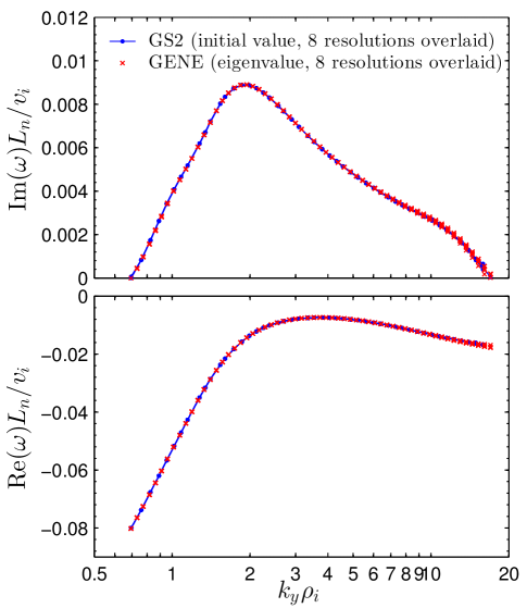
Figure 1: (Color online) Demonstration that the universal instability is numerically robust. The positive growth rate and real frequency are plotted for the unstable range of $k_{y}$ using calculations from two independent codes – gs2 run as an initial-value simulation and gene run as a direct eigenvalue solver – with results agreeing to high precision. For each code, results from many different numerical resolutions are overlaid in the figure. A reduced mass ratio $m_{i}/m_{e}=25$ is used here to further minimize the possibility of numerical artifacts.

IV Mode properties

Figure 2 displays the dependence of the frequency and growth rate on perpendicular wavenumber and magnetic shear, this time using the true deuterium-electron mass ratio. As one expects from the zero-shear universal instability, the phase velocity direction is $\mathrm{Re}(\omega/\omega_{*})>0$ (appearing in the figures as $\mathrm{Re}(\omega)<0$ due to the codes’ sign convention). The frequency satisfies $|\omega L_{n}/v_{i}|\ll 1$ and $|\omega/\omega_{*}|\ll 1$. The growth rate is smaller in magnitude than the real frequency.

When $L_{s}/L_{n}\gg 1$, instability is found for $k_{y}\rho_{i}>0.7$, extending beyond $k_{y}\rho_{i}>100$ for the highest values of $L_{s}/L_{n}$. Stability for $k_{y}\to\infty$ can be understood from the fact that $J_{0s}$ in (1)-(2) becomes small, as the gyro-motion averages out very small-scale fluctuations. Stability is the opposite limit of small $k_{y}$ is expected since Refs. Tsang et al. (1978); Ross and Mahajan (1978) are valid there. A region of stability also exists around $k_{y}\rho_{i}\approx 2$ when a realistic mass ratio is used. No such notch in the growth rate is found when the shear is exactly zero. This abrupt change in eigenvalue when a small change is made to the physical system – in this case the addition of small magnetic shear for $k_{y}\rho_{i}\approx 2$ – is a phenomenon seen in many systems with non-orthogonal eigenmodes Trefethen and Embree (2005) such as this one. For such “non-normal” systems, the behavior over a finite time is typically a much less sensitive function of parameters than the eigenvalues, which represent behavior for $t\to\infty$ when all points along the field line have had time to communicate. Indeed, in initial-value computations we find no notch near $k_{y}\rho_{i}\approx 2$ in the growth for short times $t\lesssim L_{s}/v_{i}$, before ions have have traveled far enough in $z$ to “realize” there is shear; these results will be presented in a separate publication.

Instability is found for at least some values of $k_{y}$ whenever $L_{s}/L_{n}$ exceeds a critical value of $\sim 17$. Note that in a tokamak, $L_{s}/L_{n}\approx qR/(\hat{s}L_{n})\gg 1$ can exceed this threshold value. Here $q$ is the safety factor, $R$ is the major radius, $\hat{s}=(r/q)dq/dr$, and $r$ is the minor radius. The general trend in figure 2 of decreasing growth rate with increasing shear can be understood from the observation that in the zero-shear limit, instability is found when $|k_{||}|$ is below a $k_{\perp}$-dependent threshold. When sufficient shear is included, all of these unstable parallel wavelengths are sufficiently long for there to be a significant increase in $k_{\perp}=k_{y}\sqrt{1+(z/L_{s})^{2}}$, causing $\Phi$ to be averaged out by gyroaveraging as discussed above. For some $k_{y}\rho_{i}$ such as $\sim 7$, the growth rate does not increase monotonically with $L_{s}/L_{n}$. This effect is another example of eigenvalues being sensitive and perhaps misleading, typical in non-normal systems Trefethen and Embree (2005) such as this one, for we find the short-time amplification to increase with $L_{s}/L_{n}$ monotonically.

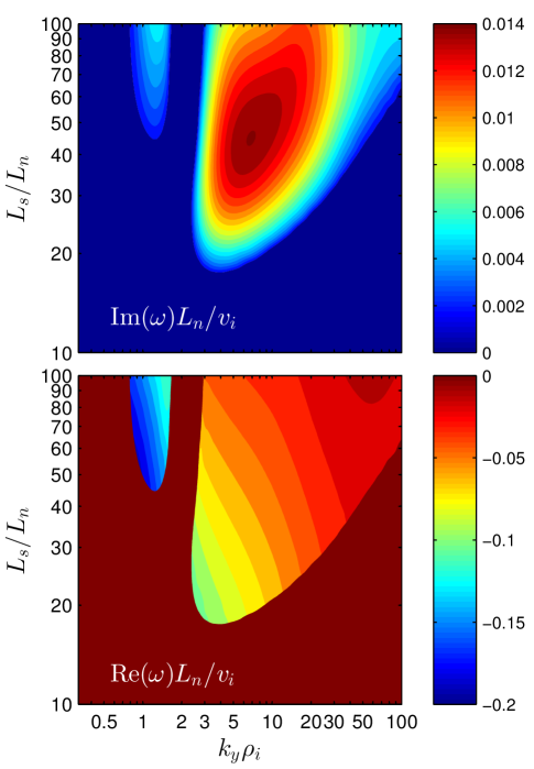
Figure 2: (Color online) Dependence of the universal instability on wavenumber and magnetic shear, for $m_{i}/m_{e}=3600$. Calculations are performed with the gs2 code.

A typical unstable eigenmode is shown in figure 3. This example is obtained using gs2 at $L_{s}/L_{n}=50$ and $k_{y}\rho_{i}=10$, near the maximum growth rate in figure 2. In the field-aligned parallel coordinate $z$, the mode has a parallel extent $\sim L_{s}$. Fourier transforming, the extent of the radial eigenmode is $\lesssim\rho_{i}$. Most of the mode structure occurs where the ion $Z$ function has an argument of order 1, $|x|\sim|\omega L_{s}/(k_{y}v_{i})|$, so the electron $Z$ function has small argument. The eigenmode amplitude is small in the inner electron region where $|x|<|\omega L_{s}/(k_{y}v_{e})|$. The electrons are highly nonadiabatic: noting the ratio of electron nonadiabatic/adiabatic terms in (4) is $\approx-(i\sqrt{\pi}/2)(L_{s}/L_{n})(\rho_{e}/\rho_{i})(\rho_{i}/|x|)$, then the nonadiabatic electron term exceeds the adiabatic term wherever $|x|<0.7\rho_{i}$, everywhere the eigenfunction is significant.

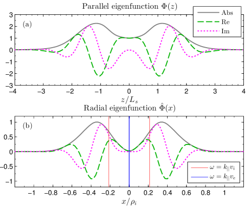
Figure 3: (Color online) Eigenmode computed with gs2 for $L_{s}/L_{n}=50$, $m_{i}/m_{e}=3600$, and $k_{y}\rho_{i}=10$ (near the maximum growth rate in figure 2). In (b), noting $k_{||}=k_{y}x/L_{s}$, vertical lines indicate the values of $x$ at which the arguments of the electron and ion $Z$ functions in (4) have unit magnitude.

Dependence of the instability on temperature gradients and collisionality is shown in figure 4, for the case $L_{s}/L_{n}=50$ and $m_{i}/m_{e}=3600$. Collisions (using the operator in Abel et al. (2008)) reduce the growth rate, particularly at the highest $k_{y}$ values. This behavior is expected because (i) in the free energy moment of (1) (Eq (222) of Abel et al. (2013)) collisions provide an energy sink; (ii) the gyrokinetic collision operator Abel et al. (2008) contains terms $\propto k_{\perp}^{2}$; and (iii) the modes at highest $k_{y}$ have fine velocity-space structure (as high resolution in energy and pitch-angle is required for numerical convergence) which collisions destroy. For sufficient collisionality, $\nu_{ee}\sim 0.05v_{i}/L_{n}$ or more, the mode is stabilized at all $k_{y}$ (for this $L_{s}/L_{n}$).

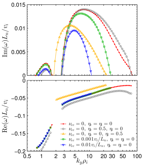
Figure 4: (Color online) Growth rate and real frequency vs. wavenumber for $L_{s}/L_{n}=50$ and $m_{i}/m_{e}=3600$, showing trends with $\eta_{s}=(d\ln T_{s}/dx)/(d\ln n_{s}/dx)$ and collisionality.

V Relationship to previous work

Let us now examine in greater detail why we find instability whereas previous authors found stability. First, consider Ref. Antonsen, Jr. (1978), which gave an analytical proof of stability in the limit $T_{i}\ll T_{e}$. We find no contradiction using gyrokinetic simulations, obtaining instability only when $T_{i}/T_{e}$ is not small. (Recall $T_{i}=T_{e}$ for all figures here.)

Next, consider Refs. Ross and Mahajan (1978); Tsang et al. (1978). These authors considered a differential eigenvalue equation, not equivalent to (4), derived assuming

$$\rho_{i}^{2}|\hat{\Phi}^{-1}\partial^{2}\hat{\Phi}/\partial x^{2}|\ll 1$$ (6)

(see e.g. Rosenbluth and Catto (1975).) No such assumption was made in deriving (4), which is therefore more general. Considering the typical eigenmode in figure 3.b, there is structure on scales smaller than $\rho_{i}$, violating (6). Therefore the approach used in Refs. Ross and Mahajan (1978); Tsang et al. (1978) is inapplicable for the modes that are unstable.

Ref. Lee et al. (1980) claims to give a proof of stability which does not rely on (6). However, this reference uses an integral eigenmode equation which differs from (4), so it is not surprising that we reach different conclusions. The eigenmode equation in Lee et al. (1980) is effectively a WKB approximation, the zero-shear dispersion relation but with $k_{x}$ replaced by $-i\,d/dx$. This WKB approximation is not justified for modes such as the one in figure 3, in which the wavelengths in $x$ are comparable to or much longer than the scale of variation in the ion and electron $Z$ functions. The problems with the integral equation in Lee et al. (1980) are discussed in the introduction of Chen et al. (1982) and references therein.

Ref Chen et al. (1982) appears to give a proof of stability using the full gyrokinetic integral eigenmode equation (4). Although we retain $J_{0e}$ for all numerical results shown here while $J_{0e}$ is set to 1 in Ref. Chen et al. (1982), this difference is unimportant: we find little change in the instability for $k_{y}\rho_{i}<20$ if $J_{0e}$ is set to 1 in gs2. The proof in Chen et al. (1982) is accomplished by multiplying the electron nonadiabatic term in (4) ($\propto 1-\omega_{*}/\omega$) by a parameter $\lambda$. The authors first prove stability in the adiabatic electron limit $\lambda=0$. We do not disagree, as we find no instability numerically with adiabatic electrons. However we do disagree with the final step of the proof, where it is argued that solutions for $\omega$ cannot cross the real axis as $\lambda$ is increased from 0 to 1 to recover (4). Including $\lambda$ in gs2, we find that modes do continuously transform from damped to unstable as $\lambda$ is increased from 0 to 1. For the case $L_{s}/L_{n}=50$ and $k_{y}\rho_{i}=10$ shown in figure 3, marginal stability occurs when $\lambda=0.032$. Therefore, the problematic step in Chen et al. (1982) is item (iii) on p750. Indeed, when $\lambda>0$, a nonadiabatic electron term must be included in (38)-(55), and this term can have opposite sign to the other terms in (55), so (56) no longer follows.

VI Conclusions

In summary, we find the plasma slab with weak or moderate magnetic shear ($L_{s}/L_{n}>17$) is generally unstable at low collisionality, even when temperature gradients are weak. The density-gradient-driven electron drift wave, known to be absolutely unstable in the absence of magnetic shear Galeev et al. (1963); Krall and Rosenbluth (1965), is not stabilized at all wavelengths when small magnetic shear is introduced, counter to previous findings. This instability is seen robustly in multiple gyrokinetic codes, and occurs for $k_{y}\rho_{i}\gtrsim 1$. Previous work that apparently showed stability of the universal mode Ross and Mahajan (1978); Tsang et al. (1978); Antonsen, Jr. (1978) assumed either (6) or $T_{i}\ll T_{e}$, whereas we make neither assumption. Ref. Lee et al. (1980) employed a less accurate dispersion relation, and Chen et al. (1982) appears incorrect for nonadiabatic electrons. Though it has sometimes been assumed that an electrostatic instability seen in a gyrokinetic simulation propagating in the electron diamagnetic direction must be a trapped electron mode or electron temperature gradient mode, our results indicate neither trapped particles nor temperature gradients are necessary for instability in this phase-velocity direction. As the universal mode can indeed be absolutely unstable in the presence of magnetic shear, it should be considered alongside temperature-gradient-driven modes, trapped particle instabilities, ballooning modes, and tearing modes as one of the fundamental plasma microinstabilities.