Stretching vortices as a basis for the theory of turbulence

Abstract

Turbulent flows play an important role in many aspects of nature and technics from sea storms to transport of particles or chemicals. Transport of energy from large scales to small fluctuations is the essential feature of three-dimensional turbulence. What mechanism is responsible for this transport and how do the small fluctuations appear? The conventional conception implies a cascade of breaking vortices. But it faces crucial problems in explaining the mechanism of the breaking, and fails to explain the observed long-living structures in turbulent flows.

We suggest a new concept based on recent analysis of stochastic Navier-Stokes equation: stretching of vortices instead of their breaking may be the main mechanism of turbulence. This conception is free of the disadvantages of the cascade paradigm; it also does not need finite-time singularities to explain the observed statistical properties of turbulent flows. Moreover, the introduction of the new conception allows immediately to get velocity scaling parameters well consistent with experimental data.

Turbulent motion implies the presence of multiple vortices of different scales. The general physical conception that has been associated with turbulence since the beginning of the XX century is the conception of cascade of breaking vortices introduced by Richardson. Just as one rock falling down breaks to two pieces, then to four pieces, etc., making a rockslide, or as energetic cosmic particle produces an avalanche of elementary particles after several generations of scatterings, large eddies in turbulent flow are believed to break consequently into smaller vortices, producing turbulence (Fig. 1). In each of these processes there is a physical quantity that conserves: in the case of crushing rocks it is the total mass of each generation, in the case of cosmic particles it is the total energy. In turbulent cascade, the conserving quantity is the energy flux from larger to smaller scales. Actually, energy is passed to a flow at large scales (from moving boat in the lake, or rotating turbine in washing machine). The only scale where it is lost is small dissipation scale which is determined by viscosity of the liquid. This is ’the end of the avalanche’, turbulence ceases at this scale. Intermediate generations of vortices belong to so-called inertial range of scales, they conduct energy from larger to smaller vortices (Fig. 2).

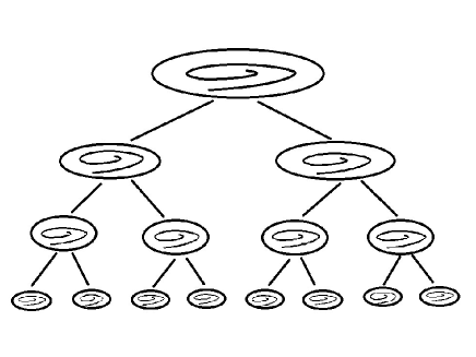
Figure 1: Cascade of breaking vortices: the well-known scheme associated with Kolmogorov’s theory (see, e.g., Frisch ) but incompatible with existence of long-living structures.

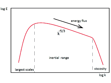
Figure 2: Kolmogorov-Richardson spectrum. The energy is pumped into the system via the largest-scale eddies, then it passes through the scales of inertial range and dissipates at viscous scale. The Kolmogorov’s theory implies that the energy dissipation (and energy flux) is independent of the Reynolds number.

This picture has inspired Kolmogorov for his K41 theory; the independence of energy flux on the scale (as viscosity tends to zero) is the central point of the theory. But the idea of the cascade of breaking vortices, though produces phenomenological base for K41, is not necessary for the rest of the theory, which is based on dimensional considerations.

Despite its illustrativeness and historical role, the conception of breaking vortices faces some problems. First, how exactly does breaking of a vortex happen? To break, a vortex should bend to make an ’8’, and reconnect the vortex lines (Fig.3). However, the process of reconnection is governed by viscosity $\nu$, and the characteristic time of reconnection is $\sim l^{2}/\nu$, where $l$ is the characteristic width of the reconnecting region. Thus, in order this time to be much smaller than the lifetime of the whole eddy (roughly speaking, to exclude the dissociation of the whole eddy before it reconnects many times, making a cascade), one has to assume that the reconnection region is very thin; as $\nu\to 0$, this implies presence of singularities at each reconnection. The existence of finite-time singularity in solutions of the Navier-Stokes (NS) and Euler ($\nu=0$) equations, which govern a hydrodynamic flow, is an open question and a subject of many investigations. If exist, the singularities could themselves produce the observed statistical properties of turbulent flows, so the cascade conception would not be needed any more. Anyway, the existence of multiple vortex breaking depends on whether singularities of such a special type exist in a flow or not.

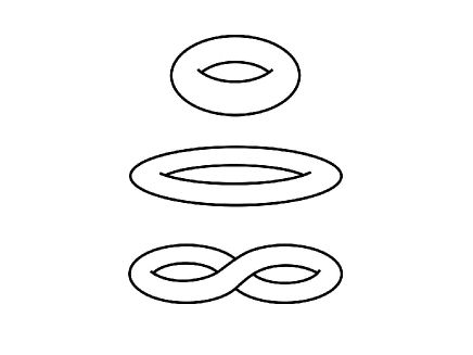
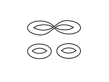
Figure 3: Breaking of a vortex. In this figure, time evolution of a typical vortex in the cascade model is shown schematically. Vortex lines are lying on the tori. To reconnect, the vortex has to become extremely thin in the vicinity of the interception. In non-viscous limit, singularity is needed to make the reconnection.

Second, many authors have reported observations of long-living ’coherent structures’ – vortex filaments – in experiments and in direct numerical simulations (DNS) (see,e.g., Frisch208vnizu or others? ). Recent investigations Farge have shown that these filaments contain the most part of helicity of the flow, and they are responsible for the observed energy spectrum corresponding to the Kolmogorov’s 5/3 law (Fig. 2). On the other hand, the lifetime of these structures exceeds many times the largest eddy turnover time; thus, their existence contradicts to the cascade conception.

If not cascade, what physical mechanism could provide the energy flux from larger to smaller scales? In the recent paper PRE13 , we have studied the solutions of the NS equation in the regions of high vorticity. We have shown that motion of particles in these regions is not just random: large-scale perturbations cause a systematic exponential stretching combined with random rotations. This stretching can be interpreted in terms of evolution of vortex filaments; moreover, it is just the process that may provide a physical picture of what happens in a turbulent flow. It allows to explain the energy flux from larger to smaller scales and to get scaling properties of statistical characteristics without any assumptions of finite-time singularities. It also may clarify the origin of the main assumption of the Kolmogorov’s theory: the energy dissipation independence of viscosity as $\nu\to 0$. Also the inequality of longitudinal and transverse statistics may be understood from this new point of view.

In what follows we first describe the main features of the observed solutions of the NS and Euler equations. Then we proceed to the statistical description and discuss the connection between the conception of stretching vortex filaments and the multifractal model (MF).

As it is shown in PRE13 , the long-time asymptote of solutions of the NS equation in the high vorticity regions can be described as random rotation and systematic exponential stretching, which corresponds to formation of a vortex filament. This stretching leads to an exponential growth of vorticity: in some special rotating coordinates, $(x,y,z)$,

$$\omega\simeq\omega_{z}=e^{ct}f\left(e^{-at}x\right)$$

Here $a<0,c>0$ are parameters (Lyapunov exponents) determined by the properties of large-scale pulsations, and $f$ is a function determined by boundary conditions near the forming filament. Independently of the particular choice of $f$, the solution ’shifts’ all the initial ripples to the center of the filament (Fig.4).

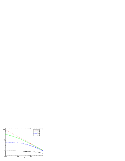
Figure 4: Evolution of vorticity distribution in one particular case:
$a=-3,c=2$, $\omega(0,x)=1/\left(1+\left[x+0.1\sin(10\pi x)\right]^{2/3}\right)$, $\omega(t,1)=1/\left(e^{-2t}+\left[1+0.1e^{-3t}\sin(10\pi e^{3t})\right]^{2/3}\right)$. One can see that the range of strong oscillations drifts to smaller $x$, while inside the ’inertial range’ the fluctuations become negligible and the power law dominates.

For any reasonable boundary condition this results in formation of a stationary (in the rotating frame!) power-law vorticity profile

$$\omega(t,x)\sim x^{c/a}\ ,$$

while the exponentially narrowing inner part remains non-stationary, and vorticity grows exponentially inside the region. This is illustrated in Fig.5. Thus, formation of vortex filaments provides scaling invariant velocity and vorticity dependencies without appearance of a finite-time singularity. In the case of small but non-zero viscosity, the growth of vorticity stops as the contraction reaches the viscous scale. If there is no viscosity, an infinite-time singularity appears in the center of the filament, instead.

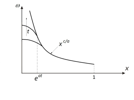
Figure 5: Illustration of vorticity distribution as a function of time inside a vortex filament: the most part of the filament has stationary power-law vorticity dependence, while the exponentially shrinking core region remains non-stationary and provides the exponential growth of the central vorticity. In the non-viscous limit, after the infinite time this would become a singularity.

However, for any finite time $t$, the velocity and vorticity distributions are smooth. The narrow non-stationary region in the center of the filament, $x<x_{0}(t)=e^{at}$ provides some non-viscous analog, or substitute, of viscosity: at $x>x_{0}(t)$, the non-viscous solution does not differ from the ’viscous’ one; the scale $x_{0}(t)$ thus has the meaning of the inner boundary of the inertial range. Although the non-viscous equation does not ’smoothen’ the initial perturbations, it transports them to smaller and smaller scales and multiplies by a decreasing term. So, the solutions of Euler and NS equations behave similarly in the limit $t\to\infty$, $\nu\to 0$.

In Kolmogorov’s theory, one assumes some definite order of taking limits: first $t\to\infty$, then $\nu\to 0$ and eventually $l\to 0$. In the model of contracting and stretching filament, one can get the same results with different order of limits: first, viscosity can be driven to zero, $\nu\to 0$; then $t\to\infty$ and finally, $l\to 0$, or $t\to\infty$ and $l\to 0$ together, but $l>x_{0}(t)$. Thus, the model is less dependent on viscosity. This simplifies understanding of the main result of the Kolmogorov’s theory even without its main assumption: even if $\nu=0$, and there is no dissipation at all, the energy flux from larger to smaller scales remains constant. Energy just continues to pass to smaller and smaller scales infinitely.

Quantitative description of turbulence implies the statistical approach. Statistical properties of a flow can be described by various correlation functions of velocity (and other related quantities). The simplest and the most widely used correlators are velocity structure functions. One distinguishes longitudinal and transverse structure functions; they are defined by

$$S_{n}^{\parallel}(l)=\left<\left|\Delta{\bf v}\cdot\frac{\bf l}{l}\right|^{n}\right>\ ,\quad S_{n}^{\perp}(l)=\left<\left|\Delta{\bf v}\times\frac{\bf l}{l}\right|^{n}\right>$$

Here $\Delta{\bf v}={\bf v}({\bf r}+{\bf l})-{\bf v}({\bf r})$ is velocity difference between two near points separated by ${\bf l}$, and the average is taken over all pairs of points separated by given $l$.

Experiments and DNS show that inside the inertial range the structure functions obey scaling laws,

$$S_{n}^{\perp}(l)\propto l^{\zeta_{n}^{\perp}}\ ,\quad S_{n}^{\parallel}(l)\propto l^{\zeta_{n}^{\parallel}}\ .$$

The scaling exponents $\zeta_{n}^{\perp}$, $\zeta_{n}^{\parallel}$ are believed to be independent on conditions of the experiment. They are intermittent, i.e., $\zeta_{n}^{\perp}/n$ and $\zeta_{n}^{\parallel}/n$ are decreasing functions of $n$.

The most successful, and nowadays conventional, way to interpret these properties is the multifractal (MF) approach introduced in ParisiFrisch . This is a generalization of Kolmogorov’s K41 theory and it allows us to express different intermittent scaling characteristics (probability densities and correlators of vorticities, accelerations, dissipation etc.) by means of one function $D(h)$. This function has the meaning of a fractal dimension of a set (’$h$-class’) near which local scale invariance holds with the scaling exponent $h$ ($\delta v\propto l^{h}$).

However, the MF model is based on dimensional consideration. Its contemporary (probabilistic) formulation does not allow us to understand what happens in a turbulent flow; the structures (or the solutions to the Navier-Stokes equation) that are responsible for the observed intermittent properties remain unknown. Intermittent behavior of the scaling exponents was obtained in Lvov2001 within the framework of the Sabra shell model, which is a simplification of the NS equation in wave-vector representation. However, the relation of the results to solutions of the NS equation remained unclear.

The idea of stretching vortices may help to fill this gap. It does not contradict to the MF model; moreover, it gives the notion of objects that contribute to correlations of each order, and to $D(h)$ (making different ’h-classes’ responsible for different scaling exponents). As we will see below, it may also help to expand the MF-model’s validity.

The question whether the longitudinal and transverse scaling exponents coincide in isotropic and homogeneous turbulence or not, is open. There is an exact statement that $\zeta_{n}^{\parallel}=\zeta_{n}^{\perp}$ for $n=2$ and 3 Frisch . On the other hand, modern experiments Zhou ; Shen and numerical simulations Chen ; Benzi show noticeable difference between $\zeta_{n}^{\parallel}$ and $\zeta_{n}^{\perp}$ at higher $n$. But the proponents of the equality argue that the difference may result from finite Reynolds number effects He ; Hill or anisotropy BifProc . Up to now, these have been the only explanations to the observed difference.

Before we continue to consider the problem, we note that isotropic and homogeneous medium does not necessarily imply $\zeta_{n}^{\perp}=\zeta_{n}^{\parallel}$. For a simple illustration, consider a gas of tops, each rotating around its own axis, the axes directions distributed randomly. Although locally a strong asymmetry could be found near each top, the whole picture remains isotropic. Vortex filaments might provide an analogous situation in real turbulence.

In terms of the MF model, two different sets of scaling exponents ($\zeta_{n}^{\parallel}$ and $\zeta_{n}^{\perp}$) correspond to two different functions $D(h)$ 25years . But the MF model is a dimensional theory, it does not distinguish longitudinal and transverse structure functions. On the other hand, the conception of stretching vortices implies that scaling exponents of different sorts and orders are contributed by different vortices. One can predict the shape of ’extreme’ vortex that provides the largest-order ($n\to\infty$) exponents: it corresponds to $h=0$ in the MF model, which means that $\delta v(l)\sim l^{0}$ According to our conception, stretching is the main process that manages the vortices, and stretching along one axis is much stronger than that in two other directions. So, the expected ’extreme’ vortex filament must have an axial symmetry and the velocity profile:

$${\bf v}=[{\bf e}_{z},{\bf r}/r]\ ,$$ (1)

We see that rotational velocity is independent of the distance $r$ to the filament’s axis $z$. The pressure diverges logarithmically in such a construction, which means that any smoother velocity profile (corresponding to infinitesimal values of $h$) is possible. (Negative values of $h$ are forbidden by infinite velocities and infinite pressure.)

Calculation of the correlators corresponding to the spatial distribution (1) gives under the limit $n\to\infty$:

$$\langle\left|\Delta v\times{\bf l}/l\right|^{n}\rangle\propto\frac{2^{n}}{n}\,l^{2}\,,\quad\langle\left|\Delta v\cdot{\bf l}/l\right|^{n}\rangle\propto n^{-5/2}l^{2}$$ (2)

The proportionality to $l^{2}$ is caused by the axial geometry of the filament (integrating $rdr$). This corresponds to the definition of $D$ given in, e.g., Frisch : the probability that at least one of a pair of points would get inside the filament is proportional to $l^{2}$. Thus, we get

$$D^{\perp}(0)=1\ ,\quad\zeta_{n}^{\perp}=2$$ (3)

However, while the contribution of the filament (2) to the transverse structure functions increases and becomes determinative as $n\to\infty$, its contribution to $\zeta_{n}^{\parallel}$ decreases because of the diminishing pre-exponential multiplier. Indeed, the ’extremely cylindric’ vortex does not produce longitudinal velocity differences.

There must be other solutions to the Euler equation to determine the behavior of $D^{\parallel}(h)$ for small $h$ and, equivalently, to make the most contribution to $S_{n}^{\parallel}$ for large $n$. Curvature of the ’extreme cylinder’ provides a subleading term differing by $l/L$ where $L$ is the curvature radius of the filament; for longitudinal structure functions, this subleading term becomes the main term. Thus, the needed solutions correspond to ’strongly curved’ extreme filament. To satisfy $h=0$, velocity must be independent of $r$. It may, for example, take the form ${\bf v}=(v_{r}(\theta),v_{\theta}(\theta),0)$ in spherical coordinates. Such a solution exists but it cannot be written analytically. Since $\delta v\sim l^{0}$ in the case, and averaging includes $r^{2}dr$, the correlator is proportional to $l^{3}$. This corresponds to

$$D^{\parallel}(0)=0\ ,\quad\zeta_{n}^{\parallel}=3$$ (4)

The difference between the boundary values (3) and (4) determines the difference between the functions $\zeta_{n}^{\perp}$ and $\zeta_{n}^{\parallel}$.

By construction, the function $D(h)$ must be growing and concave function of $h$ in the range $0\leq h\leq h_{min}$. The universal condition $\zeta_{0}^{\perp,\parallel}=0$ gives the restriction $\max\limits_{h}{D(h)}=3$. One more fundamental restriction for $D(h)$ comes from the Kolmogorov’s 4/5 law: $\zeta_{3}^{\perp,\parallel}=1$. Now as we have the boundary values $D^{\perp}(0)$ and $D^{\parallel}(0)$, we can estimate the rest of $D(h)$ just assuming it to be a parabola. Doing this leads to

$$\begin{array}[]{ll}\zeta_{n}^{\parallel}=&\left\{\begin{array}[]{lr}0.367n-1.12\cdot 10^{-2}n^{2}\ ,&\quad n\leq 16.3\ ;\\ 3\ ,&\quad n>16.3\ .\end{array}\right.\\ \zeta_{n}^{\perp}=&\left\{\begin{array}[]{lr}0.391n-1.91\cdot 10^{-2}n^{2}\ ,&\quad n\leq 10.2\ ;\\ 2\ ,&\quad n>10.2\ .\end{array}\right.\end{array}$$ (5)

In Fig. 6 we compare this theoretical prediction with the DNS data by Benzi and Gotoh . We see that the result of our simple model is very close to the experimental results and lies inside the error bars of the experiments.

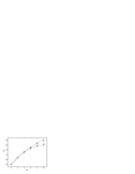
Figure 6: Euler longitudinal (upper branch) and transverse (lower branch) scaling exponents: the results of DNS from Benzi ($\bigcirc$, $\square$) and Gotoh ($\bigtriangleup$. $\bigtriangledown$), and the prediction of the theory (5) (lines).

Our simple model has one difficulty: the two parabolas plotted in Fig. 6 coincide at $n=0$ and $n=3$, hence they do not coincide at $n=2$. This contradicts to the exact theoretical statement that $\zeta_{2}^{\parallel}=\zeta_{2}^{\perp}$. However, this difficulty is caused by postulating the simplest parabolic shape for $D(h)$. It can easily be eliminated by assuming (at least one of the two) $D(h)$ to be a cubic polynomial. Because of very small divergence ($1.6\cdot 10^{-2}$) between $\zeta_{2}^{\parallel}$ and $\zeta_{2}^{\perp}$ in Fig. 6, the coefficient by the eldest order must be very small ( $\leq 10^{-4}$). It would change very slightly (unnoticeable for an eye) the lines presented in Fig. 6. The only thing it may change significantly is the rate of approaching the constant at large (but still intermediate) $n$ (from 10 to 15, approximately). But this range of $n$ is, anyway, badly described by the lowest-order polynomials: adding more degrees of freedom with very small coefficients, though unimportant for smaller $n$, would change the solutions for these $n$. However, the changes cannot be very big, since the exponents are still restricted by the values 2 and 3, respectively.

This saturation of the scaling exponents as $n\to\infty$ is an exact prediction of our model. This agrees well with Yakhot2001 where the possibility of saturation of $\zeta_{n}$ was also noticed. Saturation seems to be a typical feature of turbulent scaling exponents: the same property is demonstrated in the passive scalar theory Falkovich .

One more comment is that, knowing $D(h)$, one can use the MF model to calculate, e.g., the probability distribution function of velocity gradients or accelerations. In 25years it is shown that once $D(h)$ fits $\zeta_{n}$ well, it would also fit well the other quantities.

So, the conception of stretching vortices agrees well with the MF model and the observed statistical properties of hydrodynamic turbulence. The change of conception itself, without any additional assumptions, allows to realize what are the ’extreme’ structures contributing to the highest-order correlators: the result of vortex breaking is indefinite, whereas the result of vortex stretching is predictable. The conception of stretching vortices thus immediately leads to verifiable predictions: it implies inequality of longitudinal and transverse velocity scaling exponents and their saturation at the values 3 and 2, correspondingly.

We thank Prof.A.V. Gurevich for his kind interest to our work. The work was partially supported by RAS Programm 19 $\Pi$ ”Fundamental Problems of Nonlinear Dynamics in mathematics and physics”

References

- (1) U. Frisch, Turbulence. The legacy of A.N. Kolmogorov, Cambridge Univ. Press, Cambridge, 1995
- (2) Z.S.She, E.Jackson, S.A.Orszag, Structure and dynamics of homogeneous turbulence: models and simulations, Proc.R.Soc.Lond.A 434,101 (1991)
- (3) N. Okamoto, K. Yoshimatsu, K. Schneider, M. Farge, Y. Kaneda, Coherent vortices in high resolution direct numerical simulation of homogeneous isotropic turbulence: A wavelet viewpoint, Phys.Fluids 19 (11), 115109 (2007)
- (4) K.P. Zybin, V.A. Sirota, Multifractal structure of fully developed turbulence, Phys.Rev.E 88, 043017 (2013)
- (5) G. Parisi, U. Frisch, On the singularity structure of fully developed turbulence, in: Turbulence and Predictability in Geophysical Fluid Dynamics, Proceed. Intern. School of Physics ’E.Fermi’, 1983, Varenna, Italy; North-Holland, Amsterdam edited by. M. Ghil, R. Benzi, and G. Parisi 84-87, 1985.
- (6) V.S. L vov, A. Pomyalov, and I. Procaccia, Outliers, extreme events, and multiscaling, Phys.Rev. E, 63, 056118 (2001)
- (7) T.Zhou, R.A.Antonia, Reynolds number dependence of the small-scale structure of grid turbulence, J.Fluid Mech. 406, 81-107 (2000)
- (8) X.Shen, Z.Warhaft, Longitudinal and transvers structure functions in sheared and unsheared wind-tunnel turbulence, Phys.Fluids 14,370 (2002)
- (9) S.Chen, K.R.Sreenivasan, M.Nelkin, N.Cao, Refined similarity hypothesis for transverse structure functions in fluid turbulence, Phys.Rev.Lett. 79, 2253-2256 (1997)
- (10) R.Benzi, L.Biferale, R.Fisher, D.Q. Lamb and F. Toschi, Inertial range Eulerian and Lagrangian statistics from numerical simulations of isotropic turbulence, J.Fluid. Mech. 653, 221 (2010)
- (11) G.He, S.Chen, R.H.Kraichnan, R.Zhang, Y.Zhou, Statistics of dissipation and enstrophy induced by localized vortices, Phys.Rev.Lett 81, 4636-4639 (1998)
- (12) R.J.Hill, Equations relating structure functions of all orders, J.Fluid Mech. 434, 379 (2001)
- (13) L. Biferale, I. Procaccia, Anisotropy in Turbulent Flows and in Turbulent Transport, Phys. Rep. 414 (2-3), 43 (2005)
- (14) G. Boffetta, A. Mazzino and A. Vulpiani, Twenty-five years of multifractals in fully developed turbulence: a tribute to Giovanni Paladin. Journal of Physics A 41, 363001 (2008)
- (15) T. Gotoh, D. Fukayama, T. Nakano, Velocity field statistics in homogeneous steady turbulence obtained using a high-resolution direct numerical simulation, Phys. Fluids 14, 1065 (2002)
- (16) V. Yakhot, Mean-field approximation and a small parameter in turbulence theory, Phys.Rev.E 63,026307 (2001)
- (17) G. Falkovich, K. Gawedzki, M. Vergassola, Particles and fields in fluid turbulence, Rev. Mod. Phys. 73(4), 913-975 (2001)