Non-Perturbative Calculation of the Scalar Yukawa Theory in Four-Body Truncation

Abstract

The quenched scalar Yukawa theory is solved in the light-front Tamm-Dancoff approach including up to four constituents (one scalar nucleon, three scalar pions). The Fock sector dependent renormalization is implemented. By studying the Fock sector norms, we find that the lowest two Fock sectors dominate the state even in the large-coupling region. The one-body sector shows convergence with respect to the Fock sector truncation. However, the four-body norm exceeds the three-body norm at the coupling $\alpha\approx 1.7$.

1 Introduction

Light-Front (LF) Hamiltonian theory is a natural ab initio framework to study the structure of hadrons and strong interaction physics (see, e.g., Ref. [1] and references therein). One of the challenges of any non-perturbative quantum field theory is to develop non-perturbative renormalization schemes [2; 3; 4; 5]. In recent years, the Fock sector dependent renormalization (FSDR) has emerged as a promising systematic non-perturbative renormalization scheme and has been successfully applied to various field theory models [6; 7; 8; 9]. The idea of using sector dependent counterterms in LF dynamics was first introduced, together with the LF Fock sector truncation (also known as the LF Tamm-Dancoff), by Perry et al. in Ref. [10]. The authors argued that sector dependence is needed to compensate for the non-localities introduced by the Fock sector truncation. The use of sector dependent counterterms, based on the analysis in the explicitly covariant LF dynamics (CLFD, see Ref. [11] for a review), ensures the exact cancellation of sub-divergences appearing in the Fock sectors [7].

Here we apply the LF Hamiltonian method with FSDR to the scalar Yukawa theory. The theory can be used to model the pion mediated nucleon-nucleon interaction. The Lagrangian of the theory reads,

$$\mathscr{L}=\partial_{\mu}N^{\dagger}\partial^{\mu}N-m^{2}|N|^{2}+{{\frac{1}{2}}}\partial_{\mu}\pi\partial^{\mu}\pi-{{\frac{1}{2}}}\mu^{2}\pi^{2}+g_{0}|N|^{2}\pi+\delta m^{2}|N|^{2},$$ (1)

where $g_{0}$ is the bare coupling and $\delta m^{2}$ is the mass counterterm of the field $N(x)$. The physical coupling is denoted as $g$. It is convenient to introduce a dimensionless coupling $\alpha=\frac{g^{2}}{16\pi m^{2}}$. We use a Pauli-Villars particle with mass $\mu_{1}$ to regularize the UV divergences in the theory [12]. For brevity, we will refer to the fundamental degrees of freedom (d.o.f.) $N(x)$ and $\pi(x)$ as nucleon and pion respectively. The scalar cubic interaction is known to exhibit a vacuum instability [13]. Following Ref. [14], we adopt the “quenched approximation”, i.e., we exclude the anti-nucleon d.o.f. Previously, the Yukawa theory with FSDR has been solved up through the three-body truncation in LF dynamics [7; 8; 9], where the renormalization has already become non-trivial. Here we extend the non-perturbative calculation to the quenched four-body truncation, which further demonstrates the scalability of the FSDR scheme. Furthermore, by comparing with lower Fock sector truncations, we investigate the convergence of the Fock sector expansion.

In Sect. 2, we introduce our formalism. A set of coupled integral equations will be derived. Numerical results are presented in Sect. 3. We summarize in Sect. 4.

2 Formalism

In LF dynamics, the physical states can be obtained from the eigenvalue equation,

$$P^{+}\hat{P}^{-}{\left.|\psi(p)\right>}=M^{2}{\left.|\psi(p)\right>},$$ (2)

where $P^{+}$ is the longitudinal momentum of the system and $\hat{P}^{-}$ is the LF Hamiltonian operator. Thanks to the transverse boost invariance in LF dynamics, we have taken the total transverse momentum $\bm{P}=0$ without the loss of generality. In the Fock space, the state vector can be represented as,

$${\left.|\psi(p)\right>}=\sum_{n}\int D_{n}\;\psi_{n}(\bm{k}_{1},x_{1},\cdots\bm{k}_{n},x_{n};p){\left.|\bm{k}_{1},x_{1},\cdots\bm{k}_{n},x_{n}\right>},$$ (3)

where $\psi_{n}(\bm{k}_{1},x_{1},\cdots\bm{k}_{n},x_{n};p)\equiv\left<\bm{k}_{1},x_{1},\cdots\bm{k}_{n},x_{n}|\psi(p)\right>$ is the light-front wave function (LFWF) that depends on the longitudinal momentum fractions $x_{i}\equiv\frac{k_{i}^{+}}{P^{+}}$ and the relative transverse momenta $\bm{k}_{i}$, and $D_{n}$ stands for $2(2\pi)^{3}\delta^{(2)}(\bm{k}_{1}+\cdots\bm{k}_{n})\delta(x_{1}+\cdots x_{n}-1)\prod_{i=1}^{n}\frac{\mathrm{d}^{2}k_{i}\mathrm{d}x_{i}}{(2\pi)^{3}2x_{i}}.$ The LFWFs are normalized to unity, $\sum_{n}I_{n}=1$, where

$$I_{n}=\frac{1}{(n-1)!}\int D_{n}\left|\psi_{n}(\bm{k}_{1},x_{1},\cdots\bm{k}_{n},x_{n};p)\right|^{2}$$ (4)

is the probability that the system appears in the $n$-body Fock sector. Note that $\psi_{1}=\sqrt{I_{1}}$ is a constant. It is convenient to define $s_{n}\equiv(k_{1}+k_{2}+\cdots k_{n})^{2}=\sum_{i=1}^{n}\frac{\bm{k}_{i}^{2}+m_{i}^{2}}{x_{i}}$ and to work with the vertex functions $\Gamma_{n}(\bm{k}_{1},x_{1},\cdots,\bm{k}_{n-1},x_{n-1};p^{2})\equiv(s_{n}-p^{2})\psi_{n}(\bm{k}_{1},x_{1},\cdots\bm{k}_{n},x_{n};p)$. For simplicity we will omit the dependence on $p^{2}$ in $\Gamma_{n}$ for the ground state $p^{2}=m^{2}$.

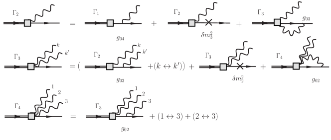
Figure 1: The diagrammatic representation of the system of equations in the four-body truncation

Truncating Eq. (2) to the four-body Fock sector gives the system of equations shown in Fig. 1. Following the LF graphical rules (see, e.g., Ref. [11]), the set of equations (after substituting $\Gamma_{4}$ into $\Gamma_{3}$) read,

$$\Gamma^{j}_{2}(\bm{k},x)=g_{04}\psi_{1}+\frac{\delta m_{3}^{2}\Gamma^{j}_{2}(\bm{k},x)}{(1-x)(s_{2}-m^{2})}+\sum_{j^{\prime}=0}^{1}(-1)^{j^{\prime}}\!\!\int\frac{{\mathrm{d}}^{2}k^{\prime}}{(2\pi)^{3}}\int_{0}^{1-x}\!\!\!\!\!\!\frac{{\mathrm{d}}x^{\prime}\;g_{03}(\xi^{\prime})}{2x^{\prime}(1-x-x^{\prime})}\frac{\Gamma_{3}^{jj^{\prime}}(\bm{k},x,\bm{k}^{\prime},x^{\prime})}{s_{3}-m^{2}},$$ (5a)

$$\Gamma^{jj^{\prime}}_{3}(\bm{k},x,\bm{k}^{\prime},x^{\prime})=Z^{(2)}((p-k-k^{\prime})^{2})\bigg{[}\frac{g_{03}(\xi^{\prime})\Gamma^{j}_{2}(\bm{k},x)}{(1-x)(s_{2}-m^{2})}+g_{02}^{2}\sum_{j^{\prime\prime}=0}^{1}(-1)^{j^{\prime\prime}}\int\frac{{\mathrm{d}}^{2}k^{\prime\prime}}{(2\pi)^{3}}\int_{0}^{1-x-x^{\prime}}$$

$$\times\frac{{\mathrm{d}}x^{\prime\prime}}{2x^{\prime\prime}(1-x-x^{\prime\prime})(1-x-x^{\prime}-x^{\prime\prime})}\frac{\Gamma^{jj^{\prime\prime}}_{3}(\bm{k},x,\bm{k}^{\prime\prime},x^{\prime\prime})}{(s_{kk^{\prime\prime}}-m^{2})(s_{4}-m^{2})}\bigg{]}+(j,\bm{k},x\leftrightarrow j^{\prime},\bm{k}^{\prime},x^{\prime}),$$ (5b)

where $$\xi^{\prime}=\frac{x^{\prime}}{1-x} \xi=\frac{x}{1-x^{\prime}} s_{2}=\frac{\bm{k}^{2}+\mu^{2}_{j}}{x}+\frac{\bm{k}^{2}+m^{2}}{1-x} s^{\prime}_{2}=\frac{\bm{k}^{\prime 2}+\mu^{2}_{j^{\prime}}}{x^{\prime}}+\frac{\bm{k}^{\prime 2}+m^{2}}{1-x^{\prime}} s_{3}=\frac{\bm{k}^{2}+\mu^{2}_{j}}{x}+\frac{\bm{k}^{\prime 2}+\mu^{2}_{j^{\prime}}}{x^{\prime}}+\frac{(\bm{k}+\bm{k}^{\prime})^{2}+m^{2}}{1-x-x^{\prime}} s_{4}=\frac{\bm{k}^{2}+\mu^{2}_{j}}{x}+\frac{\bm{k}^{\prime 2}+\mu^{2}_{j^{\prime}}}{x^{\prime}}+\frac{\bm{k}^{\prime\prime 2}+\mu^{2}_{j^{\prime\prime}}}{x^{\prime\prime}}+\frac{(\bm{k}+\bm{k}^{\prime}+\bm{k}^{\prime\prime})^{2}+m^{2}}{1-x-x^{\prime}-x^{\prime\prime}} s_{kk^{\prime\prime}}=\frac{\bm{k}^{2}+\mu^{2}_{j}}{x}+\frac{\bm{k}^{\prime\prime 2}+\mu^{2}_{j^{\prime\prime}}}{x^{\prime\prime}}+\frac{(\bm{k}+\bm{k}^{\prime\prime})^{2}+m^{2}}{1-x-x^{\prime\prime}} (p-k-k^{\prime})^{2}=m^{2}-(1-x-x^{\prime})(s_{3}-m^{2}) Z^{(n)}(q^{2})=\left(1-\frac{\Sigma^{(n)}(q^{2})-\Sigma^{(n)}(m^{2})}{q^{2}-m^{2}}\right)^{-1} Z n \Sigma^{(n)} j=0,1 \mu_{0}=\mu g_{02},g_{03},\delta m_{2}^{2},\delta m_{3}^{2} g_{03}$$, , , , , , , , and is a generalization of the -factor (the field strength renormalization constant) coming from the -body self-energy corrections . Here refers to the physical () and PV pion, respectively. As mentioned, the counterterms admit Fock sector dependence. are the two- and three-body renormalization parameters that have been obtained from the two- and three-body truncation. Note that the three-body bare coupling depends on the relative longitudinal momentum fraction, which is a consequence of the three-body truncation [7; 9].

In order to obtain the four-body bare coupling $g_{04}$, we apply the renormalization condition [7]

$$\Gamma_{2}^{j=0}(\bm{k}^{\star},x)=g\sqrt{I_{1}^{(3)}},$$ (6)

where $I_{1}^{(3)}$ is the one-body norm found in the three-body truncation and $s_{2}^{\star}\equiv\frac{{\bm{k}^{\star}}^{2}+\mu^{2}}{x}+\frac{{\bm{k}^{\star}}^{2}+m^{2}}{1-x}=m^{2}$ is on the mass shell.

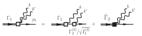
Figure 2: Split $\Gamma_{3}$ using the two-body vertex $\Gamma_{2}^{(3)}$ found in the three-body truncation

However, Eq. (5a) contains a mass pole $\frac{1}{s^{\star}_{2}-m^{2}}$, after applying the renormalization condition Eq. (6). This pole is associated with the three-body mass counterterm $\delta m_{3}^{2}$. Eq. (5) contains a similar mass pole, presumably associated with the three-body loop correction. These poles should cancel and produce a $Z$-factor when combined. To facilitate the analytical cancellation, we can split $\Gamma_{3}$ into two pieces (see Fig. 2),

$$\Gamma^{0j^{\prime}}_{3}(\bm{k},x,\bm{k}^{\prime},x^{\prime})\equiv\frac{\Gamma_{2}^{j^{\prime}(3)}(\bm{q}^{\prime},\xi^{\prime};(p-k)^{2})}{\sqrt{I^{(3)}_{1}}}\frac{\Gamma^{0}_{2}(\bm{k},x)}{(1-x)(s_{2}-m^{2})}+\widetilde{\Gamma}^{0j^{\prime}}_{3}(\bm{k},x,\bm{k}^{\prime},x^{\prime}),$$ (7)

where $\Gamma^{(3)}_{2}$ is the two-body vertex function found in the three-body truncation, $\widetilde{\Gamma}^{0j^{\prime}}_{3}(\bm{k},x,\bm{k}^{\prime},x^{\prime})$ is a regular function when $s_{2}$ is taken on mass-shell and $(p-k)^{2}=m^{2}-(1-x)(s_{2}-m^{2}),\xi^{\prime}=\frac{x^{\prime}}{1-x},\bm{q}^{\prime}=\bm{k}^{\prime}+\xi^{\prime}\bm{k}$. The first part on the right-hand side of Eq. (7) produces the necessary three-body loop correction when plugged into Eq. (5a). We substitute $\Gamma^{0j^{\prime}}_{3}$ from Eq. (7) in Eq. (5a) and then apply the renormalization condition Eq. (6). Note that thanks to FSDR, the $Z$-factor still equals the one-body norm, $Z^{(3)}\equiv\left(1-\frac{\partial}{\partial p^{2}}\Sigma^{(3)}(p^{2})\right)^{-1}_{p^{2}=m^{2}}=I_{1}^{(3)}$, even under the Fock sector truncation [8]. Then $\Gamma_{2}$ becomes,

$$\Gamma^{j}_{2}(\bm{k},x)={g}/{\sqrt{I_{1}^{(3)}}}+\delta m_{3}^{2}\frac{\Gamma^{j}_{2}(\bm{k},x)}{(1-x)(s_{2}-m^{2})}\\ +\sum_{j^{\prime}=0}^{1}(-1)^{j^{\prime}}\int\frac{{\mathrm{d}}^{2}k^{\prime}}{(2\pi)^{3}}\int_{0}^{1-x}\frac{{\mathrm{d}}x^{\prime}\;g_{03}(\xi^{\prime})}{2x^{\prime}(1-x-x^{\prime})}\left[\frac{\Gamma_{3}^{jj^{\prime}}(\bm{k},x,\bm{k}^{\prime},x^{\prime})}{s_{3}-m^{2}}-\frac{\widetilde{\Gamma}^{0j^{\prime}}_{3}(\bm{k}^{\star},x,\bm{k}^{\prime},x^{\prime})}{s_{3}^{\star}-m^{2}}\right],$$ (8)

where $s^{\star}_{3}=\frac{{\bm{k}^{\star}}^{2}+\mu^{2}}{x}+\frac{\bm{k}^{\prime 2}+\mu^{2}_{j^{\prime}}}{x^{\prime}}+\frac{(\bm{k}^{\star}+\bm{k}^{\prime})^{2}+m^{2}}{1-x-x^{\prime}}$. The on-mass-shell condition, after some arithmetic ${\bm{k}^{\star}}^{2}=-(1-x)\mu^{2}-x^{2}m^{2}$, implies that $\widetilde{\Gamma}_{3}^{0j^{\prime}}(\bm{k}^{\star},x,\bm{k}^{\prime},x^{\prime})$ is an analytic continuation of $\widetilde{\Gamma}_{3}^{jj^{\prime}}(\bm{k},x,\bm{k}^{\prime},x^{\prime})$, which can not be directly rendered in the numerical calculation. Therefore, we keep $\widetilde{\Gamma}_{3}^{0j^{\prime}}(\bm{k}^{\star},x,\bm{k}^{\prime},x^{\prime})$ as an auxiliary function that satisfies its own integral equation,

$$\widetilde{\Gamma}^{0j^{\prime}}_{3}(\bm{k}^{\star},x,\bm{k}^{\prime},x^{\prime})=Z^{(2)}((p-k^{\star}-k^{\prime})^{2})\Bigg{[}g_{02}^{2}\sum_{j^{\prime\prime}=0}^{1}\int\frac{{\mathrm{d}}^{2}k^{\prime\prime}}{(2\pi)^{3}}\int_{0}^{1-x-x^{\prime}}\!\!\!\!\!\!\!\!\!\!\!\!\!\!\!\frac{{\mathrm{d}}x^{\prime\prime}}{2x^{\prime\prime}(1-x-x^{\prime\prime})(1-x-x^{\prime}-x^{\prime\prime})}\\ \times\frac{(-1)^{j^{\prime\prime}}}{s^{\star}_{4}-m^{2}}\bigg{(}\frac{\widetilde{\Gamma}^{0j^{\prime\prime}}_{3}(\bm{k}^{\star},x,\bm{k}^{\prime\prime},x^{\prime\prime})}{s_{k^{\star}k^{\prime\prime}}-m^{2}}+\frac{\Gamma^{j^{\prime}j^{\prime\prime}}_{3}(\bm{k}^{\prime},x^{\prime},\bm{k}^{\prime\prime},x^{\prime\prime})}{s_{k^{\prime}k^{\prime\prime}}-m^{2}}\bigg{)}+\frac{g_{03}(\xi)\Gamma^{j^{\prime}}_{2}(\bm{k}^{\prime},x^{\prime})}{(1-x^{\prime})(s^{\prime}_{2}-m^{2})}\Bigg{]},$$ (9)

where $s_{k^{\star}k^{\prime\prime}}=\frac{{\bm{k}^{\star}}^{2}+\mu^{2}}{x}+\frac{\bm{k}^{\prime\prime 2}+\mu^{2}_{j^{\prime\prime}}}{x^{\prime\prime}}+\frac{(\bm{k}^{\star}+\bm{k}^{\prime\prime})^{2}+m^{2}}{1-x-x^{\prime\prime}}$, $s_{4}^{\star}=\frac{{\bm{k}^{\star}}^{2}+\mu^{2}_{j}}{x}+\frac{\bm{k}^{\prime 2}+\mu^{2}_{j^{\prime}}}{x^{\prime}}+\frac{\bm{k}^{\prime\prime 2}+\mu^{2}_{j^{\prime\prime}}}{x^{\prime\prime}}+\frac{(\bm{k}^{\star}+\bm{k}^{\prime}+\bm{k}^{\prime\prime})^{2}+m^{2}}{1-x-x^{\prime}-x^{\prime\prime}}$, $s_{k^{\prime}k^{\prime\prime}}=\frac{\bm{k}^{\prime 2}+\mu^{2}_{j}}{x^{\prime}}+\frac{\bm{k}^{\prime\prime 2}+\mu^{2}_{j^{\prime\prime}}}{x^{\prime\prime}}+\frac{(\bm{k}^{\prime}+\bm{k}^{\prime\prime})^{2}+m^{2}}{1-x^{\prime}-x^{\prime\prime}}$, and $(p-k^{\star}-k^{\prime})^{2}=m^{2}-(1-x-x^{\prime})(s^{\star}_{3}-m^{2})$.

Eqs. (5, 8, 9) constitute the properly renormalized system of equations.

3 Numerical Results

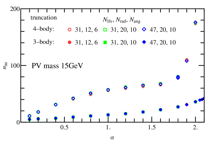
Figure 3: The number of iterations needed to achieve absolute convergence $10^{-4}$ for different couplings. Numerical difficulty is detected beyond $\alpha=1.8$

We employ an iterative method to solve the system of equations Eqs. (5, 8, 9) numerically. The vertex functions are discretized on a 5-dimensional grid. The size of the grid is proportional to $N^{2}_{\mathrm{lfx}}N^{2}_{\mathrm{rad}}N_{\mathrm{ang}}$, where $N_{\mathrm{rad}},N_{\mathrm{ang}},N_{\mathrm{lfx}}$ are the number of grid points in the transverse radial, angular and the longitudinal directions, respectively. For the integrations we use Gauss-Legendre quadrature methods, interpolating on the external grid points as necessary. We use the solution of the three-body truncation as the initial guess for the vertex functions $\Gamma$ and then update them iteratively, until they, before and after the update, satisfy the criterion $\max\big{\{}|\Gamma(\text{after})-\Gamma({\text{before}})|\big{\}}<10^{-4}$. Typically, we need 50 to 100 iterations to reach convergence (see Fig. 3).

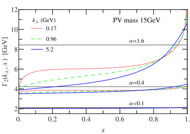
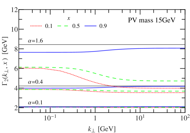
Figure 4: The two-body vertex function $\Gamma_{2}(k_{\perp},x)$ for $\alpha=0.1,0.4,1.6$, on a grid $N_{\mathrm{rad}}=47,N_{\mathrm{ang}}=N_{\mathrm{lfx}}=20$. The horizontal lines are corresponding results from the one-loop LF perturbation theory

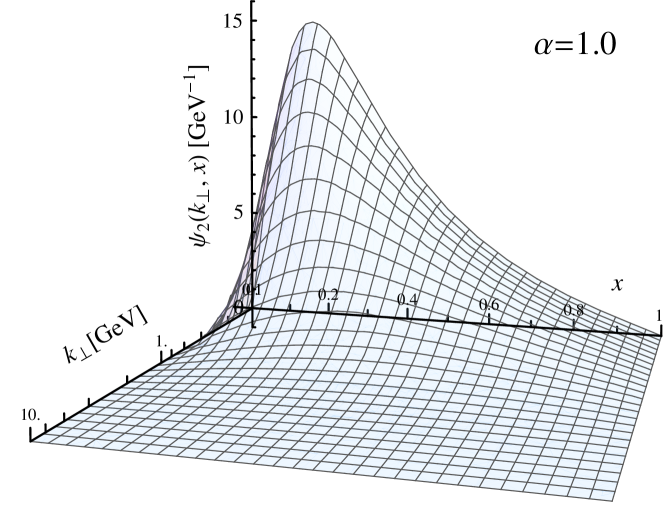
Figure 5: The two-body LFWF $\psi_{2}(k_{\perp},x)$ for $\alpha=1.0$. Grid size: $N_{\mathrm{rad}}=47,N_{\mathrm{ang}}=N_{\mathrm{lfx}}=20$

The numerical calculations were carried out on the Cray XE6 Hopper at NERSC with a hybrid MPI/OpenMP code. The system was solved at $\mu=0.14\;\mathrm{GeV},m=0.94\;\mathrm{GeV},\mu_{1}=15\,\mathrm{GeV}$ for various couplings. We have also investigated, analytically and numerically, the dependence on the PV mass as it goes to infinity. We found very weak PV mass dependence for $\mu_{1}>10\,\mathrm{GeV}$. More details will be given in Ref. [15]. Representative two-body vertex functions are shown in Fig. 4. In the one-loop LF perturbation theory, the dressed vertex is merely a constant $g$, shown as horizontal lines in Fig. 4. At small coupling, our two-body vertex function $\Gamma_{2}$ reproduces the perturbation result. From the vertex functions, we can obtain the LFWFs. Fig. 5 shows the two-body LFWF for $\alpha=1.0$.

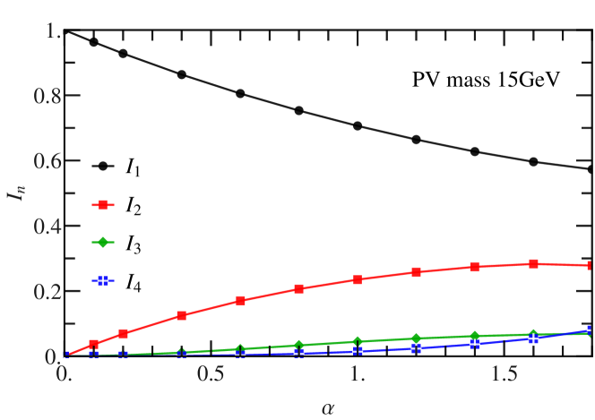
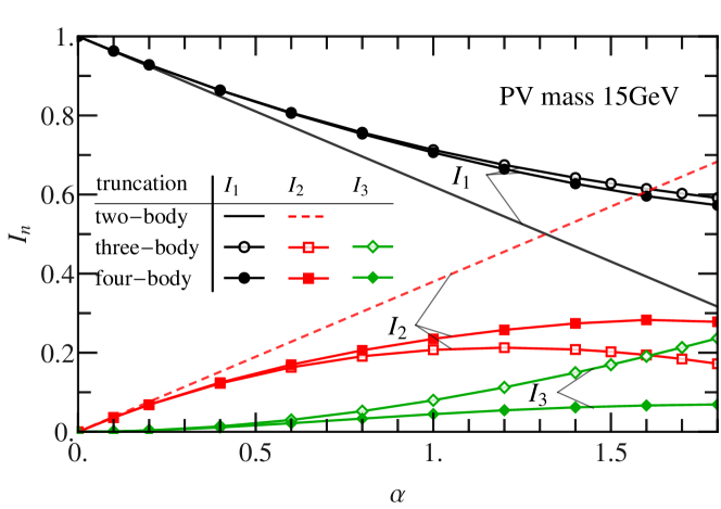
Figure 6: Top panel: the $n$-body Fock sectors norm $I_{n}$ as a function of the coupling $\alpha$ in the four-body truncation; Bottom panel: $I_{n}$ as a function of the coupling $\alpha$ in the two-, three- and four-body truncations

The top panel of Fig. 6 plots the norm of the Fock sectors (see Eq. (4)) in the four-body truncation as a function of the coupling up to $\alpha=1.8$. The contributions to the state vector show a hierarchy of Fock sectors (i.e. $I_{n}<I_{n-1}$) up to $\alpha\approx 1.7$. Beyond that $I_{4}$ becomes larger than $I_{3}$. Nevertheless, the lowest two sectors ${\left.|N\right>}+{\left.|N\pi\right>}$ are observed to dominate the Fock space up to $\alpha=1.8$, where these two sectors constitute about $85\%$ of the full norm. The bottom panel of Fig. 6 compares the four-body truncation with the two- and three-body Fock sector truncations. The one- and two-body Fock sector norm $I_{1}$ and $I_{2}$ show trend of convergence as the number of Fock sector constituents increase, especially below $\alpha\approx 1.0$. Note that the one-body sector $I_{1}$ changes little from the three-body truncation to the four-body truncation, even at large coupling. $I_{1}$ is closely related to observables, in particular, the electromagnetic form factor $F(Q^{2}\to\infty)\propto I_{1}$, and the parton distribution function of the nucleon $f(x)=I_{1}\delta(x-1)+\cdots$.

The convergence of the Fock sector truncation breaks down once the contribution of the highest Fock sector supersedes the contribution from the lower Fock sectors. In terms of the Fock sector norms, the breakdown of the two-body truncation ($I_{2}>I_{1}$) happens at $\alpha\approx 1.3$; the three-body truncation ($I_{3}>I_{2}$) at $\alpha\approx 1.6$; the four-body truncation ($I_{4}>I_{3}$) at $\alpha\approx 1.7$. This suggests that the non-perturbative results can be systematically improved by including more Fock sectors.

4 Summary

We study the scalar Yukawa theory in the non-perturbative region (up to $\alpha=1.8$) within the four-body truncation (one nucleon and three pions). The theory is quantized on the light front and a Fock sector dependent renormalization is implemented. The system of equations for the one-nucleon sector is derived and solved numerically. The investigation of the Fock sector norms largely supports the hierarchy picture up to about $\alpha\approx 1.7$: the system is dominated by the lowest Fock sectors and at a fixed coupling the Fock sector expansion shows convergence as the number of constituents increases.

The success of solving a four-body truncated quantum field theory in the non-perturbative region gives us further confidence for the use of FSDR together with LFTD as a general ab initio approach. The study of the higher Fock sector expansion in more realistic field theories such as the Yukawa model, QED and QCD models is in progress. Solving the one-nucleon sector also provides the first step to study the bound-state problem in the two-nucleon sector, which has been extensively studied in various approaches [16; 17; 18; 19]. However not all these approaches are from first principles, nor do they include a systematic non-perturbative renormalization. The investigation of this problem in the LFTD approach is also under consideration.

- [1] Bakker B. L. G., et al.: Light-Front Quantum Chromodynamics: A framework for the analysis of hadron physics. Nucl. Phys. Proc. Suppl. 251-252, 165 (2014); [arXiv:1309.6333 [hep-ph]]
- [2] Perry R. J. and Harindranath A.: Renormalization in the light-front Tamm-Dancoff approach to field theory. Phys. Rev. D 43, 4051 (1991)
- [3] Głazek S. D. and Wilson K. G.: Renormalization of Hamiltonians. Phys. Rev. D 48, 5863 (1993)
- [4] Paston S. A. and Franke V. A.: Comparison of quantum field perturbation theory for the light front with the theory in Lorentz coordinates, Theor. Math. Phys. 112, 1117 (1997) [Teor. Mat. Fiz. 112, 399 (1997)]
- [5] Grangé P., Mathiot J.-F., Butet B. and Werner W.: Taylor-Lagrange renormalization scheme: Application to light-front dynamics, Phys. Rev. D 80, 105012 (2009)
- [6] Hiller J. R. and Brodsky S. J.: Nonperturbative renormalization and the electron’s anomalous moment in large- QED. Phys. Rev. D 59, 016006 (1998); [arXiv:hep-ph/9806541]
- [7] Karmanov V. A., Mathiot J.-F, Smirnov A. V.: Systematic renormalization scheme in light-front dynamics with Fock space truncation. Phys. Rev. D 77, 085028 (2008); [arXiv:0801.4507 [hep-th]]
- [8] Karmanov V. A., Mathiot J.-F., Smirnov A. V.: Nonperturbative calculation of the anomalous magnetic moment in the Yukawa model within truncated Fock space. Phys. Rev. D 82, 056010 (2010)
- [9] Karmanov V. A., Mathiot J.-F., Smirnov A. V.: Ab initio nonperturbative calculation of physical observables in light-front dynamics: Application to the Yukawa model. Phys. Rev. D 86, 085006 (2012)
- [10] Perry R. J., Harindranath A., and Wilson K. G.: Light-Front Tamm-Dancoff field theory. Phys. Rev. Lett. 65, 2959 (1990)
- [11] Carbonell J., Desplanques B., Karmanov V. A., and Mathiot J.-F.: Explicitly Covariant Light-Front Dynamics and Relativistic Few-Body Systems. Phys. Rep. 300, 215 (1998); [arXiv:nucl-th/9804029]
- [12] Brodsky S. J., Hiller J. R., and McCartor G.: Application of Pauli-Villars regularization and discretized light-cone quantization to a single-fermion truncation of Yukawa theory. Phys. Rev. D 64, 114023 (2001)
- [13] Gordon Baym: Inconsistency of cubic boson-boson interactions. Phys. Rev. 117, 886 (1960)
- [14] Gross F., Şavklı C., and Tjon J.: Stability of the scalar interaction. Phys. Rev. D 64, 076008 (2001)
- [15] Li Y., Karmanov V. A., Maris P., Vary J. P., manuscript in preparation
- [16] Wivoda J. J., Hiller J. R.: Application of discretized light-cone quantization to a model field theory in 3+1 dimensions. Phys. Rev. D 47, 4647 (1993)
- [17] Şavklı C., Tjon J., and Gross F.: Feynman-Schwinger representation approach to nonperturbative physics, Phys. Rev. C 60, 055210 (1999); [arXiv:hep-ph/9906211]
- [18] Hwang, Dae Sung and Karmanov V. A.: Many-Body Fock sectors in Wick-Cutkosky model. Nucl. Phys. B 696, 413 (2004); [arXiv:hep-th/0405035]
- [19] Ji, Chueng-Ryong and Tokunaga, Yukihisa: Light-Front dynamic analysis of bound states in a scalar field model. Phys. Rev. D 86, 054011 (2012); [arXiv:1205.3812 [nucl-th]]