Capacity of a Simple Intercellular Signal Transduction Channel

Abstract

We model biochemical signal transduction, based on a ligand-receptor binding mechanism, as a discrete-time finite-state Markov channel, which we call the BIND channel. We show how to obtain the capacity of this channel, for the case of binary output, binary channel state, and arbitrary finite input alphabets. We show that the capacity-achieving input distribution is IID. Further, we show that feedback does not increase the capacity of this channel. We show how the capacity of the discrete-time channel approaches the capacity of Kabanov’s Poisson channel, in the limit of short time steps and rapid ligand release.

I Introduction

I-A Overview

Research at the intersection of biology and information theory stretches back almost to Shannon’s founding papers, with notable work by Yockey [1, 2], Attneave [3], Barlow [4], and Berger [5]. After long remaining on the margins of the wider information theory community, this research area finds itself newly in the limelight due to the convergence of two recent trends. First, quantitative biologists increasingly apply information-theoretic methods to the analysis of high throughput, individually resolved laboratory data [6, 7]; second, “mainstream” information theorists increasingly explore biological applications (e.g., [8, 9, 10, 11, 12]), obtaining results in fields such as molecular biology and neuroscience. These two trends have developed alongside increasing interest in the mathematical and conceptual foundations of biology, as well as interest in biologically-inspired communication systems [13, 14], further accentuating the importance of information theory in biology.

The current paper focuses on communication systems that employ chemical principles, broadly known as molecular communication [15]. Recent work in molecular communication can be divided into two categories. In the first category, work has focused on the engineering possibilities: to exploit molecular communication for specialized applications, such as nanoscale networking [15, 16]. In this direction, information-theoretic work has focused on the ultimate capacity of these channels, regardless of biological mechanisms (e.g., [12, 11]). In the second category, work has focused on analyzing the biological machinery of molecular communication (particularly ligand-receptor systems), both to describe the components of a possible communication system [17] and to describe their capacity [18, 19, 20, 8, 21]. Our paper, which builds on work presented in [19], fits into the second category, and many tools in the information-theoretic literature can be used to solve problems of this type. Related work is also found in [20], where capacity-achieving input distributions were found for a simplified “ideal” receptor; that paper also discusses but does not solve the capacity for the channel model we use.

Our contribution in this paper is to prove several important properties of capacity for a two-state signal transduction channel, which we refer to as the “Binding IN Discrete time” (BIND) channel, as found in the Dictyostelium model organism [22, 23] as well as in models of neural communication systems taking into account refractoriness or synaptic dynamics [24], [25]. The BIND channel, introduced formally in §II, is a discrete-time analog of a ubiquitous biochemical signal-transduction mechanism, described in §I-B. We show that the capacity-achieving input distribution of the BIND channel, which is a discrete-time Markov chain model, is IID, with all the probability weight on the minimum and maximum possible ligand concentrations. Further, we show that feedback does not increase the capacity of the BIND channel. Finally, given an IID input distribution, we give a simple closed-form expression for the mutual information, which can be maximized to find capacity. In addition to the capacity results, we discuss the mutual information of the BIND channel when the channel inputs are Markov distributed, and we compare our capacity results to earlier known results on the capacity of Poisson counting channels. We focus on the capacity of a single receptor, leaving the problem of multiple receptors to future work.

Indecomposable discrete time finite state channels, of which the BIND channel is an example, have been studied extensively [26]. Although the capacity is unknown for the general case, many special cases have been examined, some related to biological signaling. The trapdoor channel, introduced by Blackwell [27], has been generalized as a model for communication mediated by diffusion of chemical signals, feedback capacity and zero-error feedback capacity of which has been solved [28]. Channels with internal states provide models for systems with memory effects, intersymbol interference, or both [29, Ch. 4.6]. In some cases, the capacity of finite state channels can be increased by feedback. For example, feedback has been shown to increase the capacity for a class of finite state Markov channels in which the channel state transition probabilities are independent of the input (see, e.g., [30]). Finite state channel models for which feedback does not increase capacity are therefore of interest.

Berger, Chen, and Yin studied a general class of unit output memory (UOM) finite state channels for which feedback does not increase capacity [31, 32]. In these models, the channel state and channel output are isomorphic, and the channel output is fed back to the transmitter with unit time delay. A key feature of UOM channels is that the feedback-capacity-achieving input distribution has a simple form. As we will show in §II, the BIND model falls within this class if feedback is introduced, and we use this fact to show that the capacity and feedback capacity are the same. Relatedly, but distinctly, Permuter and colleagues introduced the Prior Output is the STate (POST) channels, a class of UOM channels for which capacity and feedback capacity may be readily evaluated [33, 34], again showing that capacity and feedback capacity are the same for many POST channels. We discuss the distinctions and relationship between the BIND and the $\text{POST}(\alpha)$ and $\text{POST}(a,b)$ channels in §V-A.

I-B Biological Motivation

As some readers of the Transactions may be unfamiliar with the details of biological signal transduction, we devote the remainder of the introduction to an overview of such systems.

Living cells communicate with one another through a web of biochemical interactions referred to as signal transduction networks[35, 36, 37]. These biochemical networks allow individual cells to perceive, evaluate and react to chemical stimuli [38, 39]. Examples include chemical signaling across the synaptic cleft connecting the axon of one nerve cell to the dendrite of another [40], calcium signaling within the postsynaptic spines of a dendrite [41], pathogen localization by migratory cells in the immune system [42], growth-cone guidance during neuronal development [43], phototransduction in the retina [44], and gradient sensing by the social amoeba Dictyostelium discoideum [45].

Signal transduction at the cellular and subcellular level typically involves a complex macromolecular apparatus comprising multiple proteins. For example, transmission of neural signals often depends on diffusion of neurotransmitter molecules across a narrow gap (the synaptic cleft) to receptor proteins on the postsynaptic membrane. These neurotransmitter receptors are connected to large protein “signaling machines” [46] that control the downstream effects of neurotransmitter signaling, including signaling mediated by the influx of extracellular calcium ions. In general, activation of a receptor will produce second messengers within the cell, which control its behaviour.

In this paper we are most interested in the process at the receiving end of signal transduction, where a signaling molecule (ligand molecule) binds to a receiver molecule (protein) at a destination cell. Despite the apparent complexity of this process, a key simplifying observation is that the receptor proteins are driven through a finite series of states by the presence of signaling molecules [47].

A two-state example, where the receptor can be either bound to the ligand (signaling) molecule or else unbound, is shown in Figure 1: if the receptor is unbound, an available ligand can bind with it, changing its state; the receptor must then go through an “unbinding” process, processing the ligand and reverting to the initial state, before it can bind with another ligand. This two-state, bound-unbound receptor model is appropriate for the 3’-5’-cyclic adenosine monophosphate (cAMP) receptor in the Dictyostelium amoeba, which is used as a model organism for studies of signal transduction [48, 49, 19]. This is the simplest nontrivial example of a ligand binding to a receptor, and forms the basis for the results in this paper.

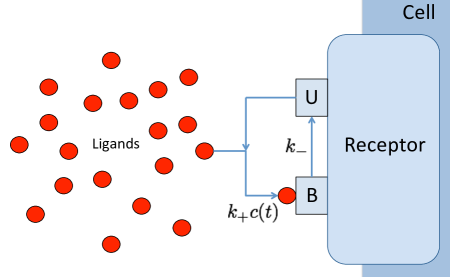
Figure 1: An example of a two-state binding and unbinding process of the receptor. If the receptor is unbound (U), then a ligand can be absorbed by the receptor; this process occurs at rate $k_{+}c(t)$, proportional to the ligand concentration $c(t)$. If the receptor is bound (B), it reverts to the unbound state at rate $k_{-}$, independent of ligand concentration.

The complexity of these systems can be much higher. In many instances, signal transduction molecules possess a number of sites at which ligand molecules can bind to the receiver protein. A protein with $k$ binding sites, each either bound or unbound, can have $2^{k}$ distinct binding states.

The signal is expressed through the time-varying concentration $c(t)$ of ligand molecules, which affects the binding rate of the receptor (as in Figure 1). We assume throughout the paper that the binding of ligand molecules to a receptor protein obeys the familiar law of mass action [50, 51], namely, that the rate of the reaction

$$\text{Ligand}+\text{Unbound Receptor}\to\text{Bound Receptor}$$ (1)

proceeds at a rate proportional to the product of the concentration of the reactants, i.e.

$$r_{\text{binding}}=k_{+}[\text{Ligand}][\text{Unbound Receptor}].$$

Here $k_{+}$ is the rate constant for the forward (binding) reaction, and [A] is the concentration of chemical species A, typically measured in nM ($10^{-9}$ moles per liter). For the cyclic AMP (cAMP) molecule binding to the cAMP receptor in the Dictyostelium amoeba, $k_{+}$ is on the order of $4\times 10^{-2}(\text{sec}\,\text{nM})^{-1}$. The reverse reaction also occurs:

$$\text{Bound Receptor}\to\text{Ligand}+\text{Unbound Receptor}$$ (2)

with rate

$$r_{\text{unbinding}}=k_{-}[\text{Bound Receptor}].$$

Ueda et al. measured the distribution of binding durations of individual cAMP receptors and found the release time following binding is well approximated by an exponential waiting time distribution with rate $k_{-}\approx 1/\text{sec}$ [52]. The law of mass action thus dictates that the concentration of bound receptors $[\mathsf{B}]$ obeys the differential equation

$$\frac{d[\mathsf{B}]}{dt}=k_{+}[\text{Ligand}][\mathsf{U}]-k_{-}[\mathsf{B}].$$ (3)

The signal available to the cell from its surroundings takes the form of the time varying ligand concentration, $c(t)=[\text{Ligand}]$. This time-varying concentration serves as the input of the channel we consider. For a given cell, the total number of bound and unbound receptors is a fixed constant, $[\mathsf{U}]+[\mathsf{B}]=[\text{Total}].$ Dividing by the total number of receptors, and setting $y(t)=[\mathsf{B}]/[\text{Total}]$ to be the fraction of receptors that are bound to ligand at time $t$, the law of mass action translates into a first order affine linear differential equation

$$\frac{dy}{dt}=k_{+}c(t)(1-y)-k_{-}y.$$ (4)

Such a differential equation is a simple example of a chemical master equation [53].

We focus now on a single receptor, binding and releasing ligand independently of the other receptors. At the single protein level mass action kinetics translates into a well established stochastic representation [54]. Let $p(t)$ be the probability that the receptor’s binding site is occupied by a ligand molecule at time $t$. Then $p(t)$ evolves according to a master equation of the same form as (4)

$$\frac{dp}{dt}=k_{+}c(t)(1-p)-k_{-}p.$$ (5)

This system may naturally be viewed as a communications channel in which the input is the time varying concentration $c(t)$, and the output is the receptor state (bound or unbound).

The BIND channel, introduced in §II, is a discrete time analog of this system. Both the continuous and discrete time versions of the ligand-binding channel share an important asymmetry. When the receptor is in the unbound state, its transition rate is sensitive to the input signal (the ligand concentration). When the receptor is in the bound state, it cannot bind a second ligand molecule until releasing the one it has already bound: the channel must leave the bound state before becoming sensitive to the input again. This asymmetry reflects the different roles of the signal in reactions (1) and (2). In the forward reaction (binding: reaction 1) the ligand is a reactant, and the rate of reaction is proportional to the ligand’s concentration. In the backward reaction (unbinding: reaction 2) the ligand is instead a product. The reaction rate is a function of the reactant concentrations, not the product concentrations, so the unbinding reaction proceeds at an instantaneous rate that does not depend on the input signal concentration. This asymmetry occurs naturally in any model of ligand-mediated biochemical signal transduction, but is absent from other binary channel models with memory, such as the trapdoor, Ising, Glenn-Elliott, or $\text{POST}(\alpha)$ channels [55, 28, 33, 27, 56]. Thus ligand-receptor binding presents a novel, and intrinsically biological, type of communications channel.

Basic mechanisms of signal transduction have been known for decades [57, 58]. However, recent technological advances have dramatically increased the ability to manipulate and measure the signals entering and leaving signal transduction networks at the molecular level. These advances create an opportunity for quantitative understanding of molecular communication. For example, microfluidics combined with cell-by-cell single track measurements have been used to estimate the mutual information between a chemical gradient and the motile response of the Dictyostelium amoeba [59, 60]. Single molecule fluorescence methods have allowed visualizing the binding and unbinding of signaling molecules to single receptors in real time [52]. High throughput measurements have led to sufficiently precise capacity estimates, for a cancer-related signaling network, to extract information about the network topology [61]. Optogenetics methods have created a new paradigm for manipulating molecular communication devices using applied light sources [62]. Thus, our results come at an opportune time for biological researchers, both in terms of their analytical capabilities and their interest in exploiting information theory. At the same time, development of novel communications models based on biological systems has been identified as an important growth area by the information theory community.

I-C Capacity problem for a general point process channel

We now introduce a general description of the continuous time signal transduction channel with arbitrary (bounded) scalar input and discrete output. Finite state Markov processes conditional on an input process provide models of signal transduction and communication in a variety of biological systems, as detailed in the preceding section. Typically, a single ion channel, or receptor, is in one of $n$ states. The states form a finite directed graph $\mathcal{Y}$ with $n$ vertices, with edges connecting states that intercommunicate through a conformational or chemical change, or ligand-binding/unbinding event. The receptor performs a continuous-time random walk on the graph, with one or more transition rates being influenced by the external input signal, $X(t)$. The input signal can be the concentration of a diffusing signaling molecule for a ligand-gated receptor; it can be the transmembrane electrical potential for a voltage-gated receptor [64].

There is a rich literature on the use of master equations for representing stochastic chemical reactions [54] and algorithms for generating sample trajectories [65, 66, 67]. In the master equation representation of a signal transduction channel, the instantaneous transition rate matrix $\mathbf{Q}=[q_{jk}]$ depends on the external input $X(t)$. The probability, $p_{k}$, that the channel is in state $Y(t)=k$ for some $k\in\mathcal{Y}$ evolves according to

$$\frac{dp_{k}}{dt}=\sum_{j=1}^{n}p_{j}(t)q_{jk}(X(t))$$ (6)

where for $(j\neq k)$, $q_{jk}\geq 0$ is the input-dependent rate at which the receptor transitions from state $j$ to state $k$, and $q_{jj}=-\sum_{k,k\neq j}q_{jk}$. Taking $\{X(t)\}_{t=0}^{T}$ as the input, and the receptor state $Y(t)\in\mathcal{Y}$ as the output, gives a channel model, the capacity of which is of general interest.

We emphasize that equation (5) corresponds to (6) in the case $n=2$. Let $\mathcal{Y}=\{\mathsf{U},\mathsf{B}\}$ be the state graph and let $p_{\mathsf{U}}$ and $p_{\mathsf{B}}$ be the probability of the receptor being in the unbound and bound states, respectively. Set

$$q_{\mathsf{U}\mathsf{B}}(c(t))=k_{+}c(t),\hskip 28.45274ptq_{\mathsf{B}\mathsf{U}}=k_{-},$$ (7)

and identify $X(t)=c(t)$ as the input signal. The correspondence follows, since the equations

$$\frac{dp_{\mathsf{B}}}{dt} =-p_{\mathsf{B}}q_{\mathsf{B}\mathsf{U}}+p_{\mathsf{U}}q_{\mathsf{U}\mathsf{B}}(X(t))$$ (8)

$$\frac{dp_{\mathsf{U}}}{dt} =p_{\mathsf{B}}q_{\mathsf{B}\mathsf{U}}-p_{\mathsf{U}}q_{\mathsf{U}\mathsf{B}}(X(t))$$ (9)

are equivalent to equation (5), given $p_{\mathsf{B}}(0)+p_{\mathsf{U}}(0)\equiv 1$.

The majority of biological signal transduction systems operate without regulation by a fast clock, i.e. they operate as continuous-time stochastic systems. Nevertheless, discrete time channel models arise as approximations to continuous time systems by fixing a small time step. While most of our analysis falls in the discrete time framework, we discuss the relation to continuous time systems further in §IV.

A related classical Poisson channel was solved by Kabanov [68, 69]. In the limit as $k_{-}\rightarrow\infty$, in which transition from the bound state back to the unbound state is instantaneous, the ligand-binding channel becomes a simple counting process, with the input encoded in the time varying intensity. This situation is exactly the one considered in Kabanov’s analysis of the capacity of a Poisson channel, under a max/min intensity constraint [68, 69]. For the Poisson channel, the capacity may be achieved by setting the input to be a two-valued random process fluctuating between the maximum and minimum intensities. If the intensity is restricted to lie in the interval $[1,1+c]$, the capacity is [69]

$$C_{\mbox{Kab}}(c)=\frac{(c+1)^{1+1/c}}{e}-\left(1+\frac{1}{c}\right)\ln(c+1).$$ (10)

As shown by Wyner [70, 71], Kabanov’s formula may be obtained (nonrigorously) by restricting the input to a two-state discrete time process with IID input $X(t)$ taking the values $X_{\text{lo}}=1$ and $X_{\text{hi}}=1+c$. In addition, Kabanov proved that the capacity of the Poisson channel cannot be increased by allowing feedback.

Kabanov’s approach, focusing on instantaneous unbinding and restricted intensity, is not directly applicable to molecular signal transduction. However, our long-term goal is to obtain expressions analogous to (10) for the continuous-time systems (5) and (6). As a first step, we restrict attention to a discrete time analog of the two-state system (5). As we show in §IV-B, our channel model can be seen as a natural generalization of Kabanov’s counting process channel model.

In the next section we define and analyze the BIND channel, a two-state signal-transduction channel model in discrete time based on ligand-mediated biochemical signal transduction, and we rigorously find its capacity.

II Capacity of the BIND channel, a discrete intercellular signal transduction channel

In this section, we introduce the BIND channel and prove our main capacity results. A roadmap for these results is given as follows:

1. In (46), we give a closed-form expression for the mutual information of the BIND channel if the inputs are IID. This expression can be maximized to find capacity with input distribution constrained to be IID (the IID capacity, see (47)), but IID capacity is not available in closed form.

2. In Theorem 1, we show that the IID capacity of the BIND channel is achieved when only the minimum and maximum possible ligand concentrations are used, and no intermediate concentration. (This theorem is given first as it simplifies the proof of the main result.)

3. In Theorem 2, we then show that capacity of the BIND channel is achieved by the IID input distribution, with inputs only on minimum and maximum ligand concentration. We do so by showing that the feedback capacity of the channel is satisfied by an IID input distribution, relying on the important results on feedback capacity from [72, 31].

4. Finally, in Corollary 1, combining Theorems 1 and 2 with Equation (47), IID capacity is given by (82). An illustration is given in Figure 3.

II-A Discrete-input, discrete-time model

The BIND channel is a discrete-time, two-state Markov channel representation of the signal reception process, an example of which may be found in the Dictyostelium cAMP receptor. The channel input, channel output, and input-output relationship are described as follows.

Channel input. The channel input is the local concentration of ligands at the receptor: at the interface between the receptor and the environment, the receptor is sensitive to the concentration of ligands, binding more frequently as concentration increases. We assume that the input concentration $c_{j}$ is one of $m$ discrete levels, and without loss of generality, we will assume $c_{1}\leq c_{2}\leq\ldots\leq c_{m}$. The lowest concentration $c_{1}$ and highest concentration $c_{m}$ are especially important in our analysis; we will give them the special symbols $c_{\mathsf{L}}:=c_{1}$ and $c_{\mathsf{H}}:=c_{m}$. Thus, the input (concentration) alphabet is

$$\mathcal{X}=\{c_{\mathsf{L}},c_{2},c_{3},\ldots,c_{m-1},c_{\mathsf{H}}\}.$$ (11)

Further, let $X_{0}^{n-1}=[X_{0},X_{1},\ldots,X_{n-1}]\in\mathcal{X}^{n}$ represent a sequence of inputs to the receptor.

Channel output. The channel output is the state of the receptor. As in Figure 1, the receptor may either be in an unbound state, in which the receptor is waiting for a molecule to bind; or in a bound state, in which the receptor has captured a molecule, and cannot capture another until the molecule is degraded or released. Thus, channel output is binary: let $\mathcal{Y}=\{\mathsf{U},\mathsf{B}\}$ represent the output alphabet, where $\mathsf{U}$ represents the unbound state and $\mathsf{B}$ represents the bound state. Further, let $Y_{1}^{n}=[Y_{1},Y_{2},\ldots,Y_{n}]\in\mathcal{Y}^{n}$ represent a sequence of receptor states. (Note the offset of index compared with $X_{0}^{n-1}$, clarified in the diagram below.)

Input-output relationship. Figure 2 illustrates the state transitions of the BIND model.

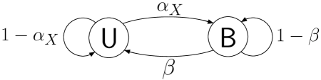
Figure 2: State transition diagram for the BIND model. Channel state $Y\in\{\mathsf{U},\mathsf{B}\}$ determines sensitivity to input ($\mathsf{U}$: Unbound receptor, sensitive to input. $\mathsf{B}$: Bound receptor, insensitive to input). Ligand concentration $c_{X}$ is the input, with $c_{\mathsf{L}}\leq c_{X}\leq c_{\mathsf{H}}$. ($c_{\mathsf{L}}$ = lowest allowed input concentration. $c_{\mathsf{H}}$ = highest input concentration.) Input binding probability $\alpha_{X}=k_{+}c_{X}\Delta t$ depends on the input concentration. Unbinding probability $\beta=k_{-}\Delta t$ is independent of input concentration.

The dependencies of the transition probabilities can be illustrated graphically as follows:

$$\begin{array}[]{ccccccccccc}&X_{0}&&X_{1}&&X_{2}&&X_{3}&&X_{4}&\cdots\\ &\downarrow&&\downarrow&&\downarrow&&\downarrow&&\downarrow\\ Y_{0}&\longrightarrow&Y_{1}&\longrightarrow&Y_{2}&\longrightarrow&Y_{3}&\longrightarrow&Y_{4}&\cdots\end{array}$$

The state of the receptor is dependent on the previous input and the previous state, forming a Markov transition PMF $p_{Y_{i}|X_{i-1},Y_{i-1}}(y_{i}\>|\>x_{i-1},y_{i-1})$. Following the discussion in the previous section, if $Y_{i-1}=\mathsf{U}$, i.e. the receptor was previously unbound, then the distribution of $Y_{i}$ depends on the input concentration $X_{i-1}$. However, if $Y_{i-1}=\mathsf{B}$, then $Y_{i}$ is independent of $X_{i-1}$.

Thus, the Markov transition PMF $p_{Y_{i}|X_{i-1},Y_{i-1}}(y_{i}|x_{i-1},y_{i-1})$ has $m+1$ parameters: the $m$-dimensional vector $\alpha=[\alpha_{1},\alpha_{2},\ldots,\alpha_{m}]$ of binding rates, where

$$\alpha_{j}:=p_{Y_{i}|X_{i-1},Y_{i-1}}(\mathsf{B}\>|\>c_{j},\mathsf{U});$$ (12)

and $\beta$, the unbinding rate, independent of input signal concentration, where

$$\beta:=p_{Y_{i}|X_{i-1},Y_{i-1}}(\mathsf{U}\>|\>c_{j},\mathsf{B})$$ (13)

which is constant for all $c_{j}\in\mathcal{X}$. This may also be written as a state transition probability matrix

$$\mathbf{P}_{Y|X=c_{j}}=\left[\begin{array}[]{cc}1-\alpha_{j}&\alpha_{j}\\ \beta&1-\beta\end{array}\right].$$ (14)

Recalling the notation from (11), we write $\alpha_{\mathsf{L}}$ and $\alpha_{\mathsf{H}}$ for the lowest and highest binding rates, respectively. Thus, we can write $\alpha=[\alpha_{\mathsf{L}},\alpha_{2},\ldots,\alpha_{m-1},\alpha_{\mathsf{H}}]$.

To relate this system to the master equation in (5), time is discretized into steps of length $\Delta t$. The parameters $\alpha$ and $\beta$ are then obtained from the rates $k_{+}$ and $k_{-}$ via $\alpha_{i}=k_{+}c_{i}\Delta t$, and $\beta=k_{-}\Delta t$. The time step $\Delta t$ has to be small enough that $\mathbf{P}_{Y|X=c_{j}}$ is a valid transition probability matrix.

From the above discussion, the sequence $Y_{1}^{n}$, given $X_{1}^{n}$ and initial input/output pair $X_{0},Y_{0}$, forms a time-inhomogeneous Markov chain with PMF

$$p_{Y_{1}^{n}|X_{0}^{n-1},Y_{0}}(y_{1}^{n}\>|\>x_{0}^{n-1},y_{0})=\prod_{i=1}^{n}p_{Y_{i}|X_{i-1},Y_{i-1}}(y_{i}\>|\>x_{i-1},y_{i-1}).$$ (15)

We give the following expressions and definitions, which will be useful in the remainder of this section. For an IID input distribution $p_{X}(x)$, since there are $m$ possible values for $x$, we will express $p_{X}(x)$ as a vector $p$, with elements

$$p =[p_{1},p_{2},\ldots,p_{m}]$$ (16)

$$=[p_{\mathsf{L}},p_{2},p_{3},\ldots,p_{m-1},p_{\mathsf{H}}].$$ (17)

For the IID input distribution vector $p$, let $\bar{\alpha}_{p}$ represent the average binding probability, given by

$$\bar{\alpha}_{p}=\sum_{j=1}^{m}\alpha_{j}p_{j}.$$ (18)

Finally, we give a condition on the parameters that will be used in many of our results:

Definition 1 (Strictly Ordered Parameters)

The parameters $\alpha$ and $\beta$ are said to be strictly ordered if they satisfy

$$0<\alpha_{\mathsf{L}}<\alpha_{2}<\alpha_{3}<\ldots<\alpha_{m-1}<\alpha_{\mathsf{H}}<1$$ (19)

and

$$0<\beta<1.$$ (20)

II-B Mutual information and capacity under IID inputs

Let $C$ represent the Shannon capacity of the system; as the BIND channel is a channel with memory, capacity is defined by

$$C=\lim_{n\rightarrow\infty}\max_{p_{X_{0}^{n-1}}(x_{0}^{n-1})}\frac{1}{n}I(X_{0}^{n-1};Y_{1}^{n}),$$ (21)

Let $C_{\mathrm{IID}}$ represent the capacity from (21) where $p_{X_{0}^{n-1}}(x_{0}^{n-1})$ is constrained to be IID, i.e., we can write $p_{X_{0}^{n-1}}(x_{0}^{n-1})=\prod_{i=0}^{n-1}p_{X}(x_{i})$.

If the input distribution is IID, then $Y_{1}^{n}$ forms a time-homogeneous Markov chain [31]. To see this, again assuming for convenience that $y_{0}$ is given, we start with

$$p_{Y_{1}^{n},X_{0}^{n-1}|Y_{0}}(y_{1}^{n},x_{0}^{n-1}\>|\>y_{0})$$

$$=p_{Y_{1}^{n}|X_{0}^{n-1},Y_{0}}(y_{1}^{n}\>|\>x_{0}^{n-1},y_{0})p_{X_{0}^{n-1}}(x_{0}^{n-1})$$ (22)

$$=p_{Y_{1}^{n}|X_{0}^{n-1},Y_{0}}(y_{1}^{n}\>|\>x_{0}^{n-1},y_{0})\prod_{i=0}^{n-1}p_{X}(x_{i})$$ (23)

$$=\prod_{i=1}^{n}p_{Y_{i}|X_{i-1},Y_{i-1}}(y_{i}\>|\>x_{i-1},y_{i-1})p_{X}(x_{i-1}),$$ (24)

where (24) follows from (15). Continue by letting

$$p_{Y_{i}|Y_{i-1}}(y_{i}\>|\>y_{i-1})$$

$$=\sum_{x_{i-1}}p_{Y_{i}|X_{i-1},Y_{i-1}}(y_{i}\>|\>x_{i-1},y_{i-1})p_{X}(x_{i-1}).$$ (25)

Finally, marginalizing over $X_{0}^{n-1}$,

$$p_{Y_{1}^{n}|Y_{0}}(y_{1}^{n}\>|\>y_{0})$$ (26)

$$= \sum_{x_{0}^{n-1}}p_{Y_{1}^{n},X_{0}^{n-1}|Y_{0}}(y_{1}^{n},x_{0}^{n-1}\>|\>y_{0})$$

$$= \prod_{i=1}^{n}\sum_{x_{i-1}}p_{Y_{i}|X_{i-1},Y_{i-1}}(y_{i}\>|\>x_{i-1},y_{i-1})p_{X}(x_{i-1})$$ (27)

$$= \prod_{i=1}^{n}p_{Y_{i}|Y_{i-1}}(y_{i}\>|\>y_{i-1}),$$ (28)

which is the distribution of a time-homogeneous Markov chain. If $y_{i-1}=\mathsf{U}$,

$$p_{Y_{i}|Y_{i-1}}(\mathsf{B}\>|\>\mathsf{U}) =\sum_{x_{i}}p_{Y_{i}|X_{i-1},Y_{i-1}}(\mathsf{B}\>|\>x_{i-1},\mathsf{U})p_{X}(x_{i-1})$$ (29)

$$=\sum_{j=1}^{m}\alpha_{j}p_{j}$$ (30)

$$=\bar{\alpha}_{p},$$ (31)

with $p_{Y_{i}|Y_{i-1}}(\mathsf{U}\>|\>\mathsf{U})=1-\bar{\alpha}_{p}$. If $y_{i-1}=\mathsf{B}$,

$$p_{Y_{i}|Y_{i-1}}(\mathsf{U}\>|\>\mathsf{B}) =\sum_{x_{i-1}}p_{Y_{i}|X_{i-1},Y_{i-1}}(\mathsf{U}\>|\>x_{i-1},\mathsf{B})p_{X}(x_{i-1})$$ (32)

$$=\sum_{j=1}^{m}\beta p_{j}$$ (33)

$$=\beta,$$ (34)

with $p_{Y_{i}|Y_{i-1}}(\mathsf{B}\>|\>\mathsf{B})=1-\beta$. The transition probability matrix for $Y$ is given by

$$\mathbf{P}_{Y}=\left[\begin{array}[]{cc}1-\bar{\alpha}_{p}&\bar{\alpha}_{p}\\ \beta&1-\beta\end{array}\right].$$ (35)

Suppose the parameters are strictly ordered (Definition 1). Then $Y$ has a stationary distribution, by inspection of (35). The stationary probability of state $\mathsf{U}$ is given by

$$p_{Y}(\mathsf{U})=\frac{1}{1+\bar{\alpha}_{p}/\beta},$$ (36)

and $p_{Y}(\mathsf{B})=1-p_{Y}(\mathsf{U})$.

When $Y_{1}^{n}$ is a time-homogeneous Markov chain, we can write the mutual information rate as

$$\mathcal{I}(X;Y) =\lim_{n\rightarrow\infty}\frac{1}{n}I(X_{0}^{n-1};Y_{1}^{n})$$ (37)

$$=H(Y_{i}\>|\>Y_{i-1})-H(Y_{i}\>|\>X_{i-1},Y_{i-1})$$ (38)

for any $i\in\{1,2,\ldots,n\}$. Let

$$\mathscr{H}(p)=-p\log p-(1-p)\log(1-p)$$ (39)

represent the binary entropy function. Dealing with each term on the right hand side of (38) individually,

$$H(Y_{i}\>|\>Y_{i-1})$$

$$=p_{Y}(\mathsf{U})H(Y_{i}\>|\>Y_{i-1}=\mathsf{U})+p_{Y}(\mathsf{B})H(Y_{i}\>|\>Y_{i-1}=\mathsf{B})$$ (40)

$$=p_{Y}(\mathsf{U})\mathscr{H}(\bar{\alpha}_{p})+p_{Y}(\mathsf{B})\mathscr{H}(\beta)$$ (41)

which follows from (31)-(34); and

$$H(Y_{i}\>|\>X_{i-1},Y_{i-1})$$

$$= \sum_{x_{i-1}}p_{X}(x_{i-1})p_{Y}(\mathsf{U})H(Y_{i}\>|\>X_{i-1}=x_{i-1},Y_{i-1}=\mathsf{U})$$

$$+\sum_{x_{i-1}}p_{X}(x_{i-1})p_{Y}(\mathsf{B})H(Y_{i}\>|\>X_{i-1}=x_{i-1},Y_{i-1}=\mathsf{B})$$ (42)

$$= \ p_{Y}(\mathsf{U})\sum_{j=1}^{m}p_{j}\mathscr{H}(\alpha_{j})+p_{Y}(\mathsf{B})\mathscr{H}(\beta).$$ (43)

Then the mutual information rate is given by

$$\mathcal{I}(X;Y) =H(Y_{i}\>|\>Y_{i-1})-H(Y_{i}\>|\>X_{i-1},Y_{i-1})$$ (44)

$$=p_{Y}(\mathsf{U})\left(\mathscr{H}(\bar{\alpha}_{p})-\sum_{j=1}^{m}p_{j}\mathscr{H}(\alpha_{j})\right)$$ (45)

$$=\frac{\mathscr{H}(\bar{\alpha}_{p})-\sum_{j=1}^{m}p_{j}\mathscr{H}(\alpha_{j})}{1+\bar{\alpha}_{p}/\beta}.$$ (46)

Finally, $C_{\mathrm{IID}}$ is given by

$$C_{\mathrm{IID}}=\max_{p}\frac{\mathscr{H}(\bar{\alpha}_{p})-\sum_{j=1}^{m}p_{j}\mathscr{H}(\alpha_{j})}{1+\bar{\alpha}_{p}/\beta}.$$ (47)

II-C $C_{\mathrm{IID}}$ is achieved with all probability mass on $x=\mathsf{L},\mathsf{H}$

Here we show that the $C_{\mathrm{IID}}$-achieving input distribution $p_{X}(x)$ uses only the extreme values of concentration: $\mathsf{L}$ and $\mathsf{H}$. The result is stated as follows.

Theorem 1

Let $p^{*}=[p_{1}^{*},p_{2}^{*},\ldots,p_{m}^{*}]$ represent an IID distribution that maximizes (47). If the parameters are strictly ordered (see Definition 1), then $p_{2}^{*}=p_{3}^{*}=\ldots=p_{m-1}^{*}=0$.

Proof: The proof proceeds by contradiction. Assume the theorem is false: that $p_{i}^{*}>0$ for at least one index $i$ in $\{2,3,\ldots,m-1\}$. Let $u$ represent the smallest index in $\{2,3,\ldots,m-1\}$ such that $p_{u}^{*}>0$. From the initial assumption, $u$ must exist, and $\alpha_{u}$ is the corresponding binding probability.

Since $\alpha_{1}<\alpha_{u}<\alpha_{m}$, there exist constants $\pi_{1}$ and $\pi_{m}$ such that

$$0<\pi_{1},\pi_{m} <1$$ (48)

$$\pi_{1}+\pi_{m} =1$$ (49)

$$\pi_{1}\alpha_{1}+\pi_{m}\alpha_{m} =\alpha_{u}.$$ (50)

Let $q=[q_{1},\ldots,q_{m}]$ represent a distribution constructed as follows:

$$q_{1} =p_{1}^{*}+p_{u}^{*}\pi_{1}$$ (51)

$$q_{m} =p_{m}^{*}+p_{u}^{*}\pi_{m}$$ (52)

$$q_{u} =0$$ (53)

$$q_{j} =p_{j}^{*}\>\>\>\>\forall j\neq\{1,u,m\}.$$ (54)

Note that $q$ is constructed so that $\bar{\alpha}_{q}=\bar{\alpha}_{p^{*}}$ (see (18)).

From (46), the mutual information under distribution $p^{*}$ is

$$\mathcal{I}_{p^{*}}(X;Y)=\frac{\mathscr{H}(\bar{\alpha}_{p^{*}})-\sum_{i=1}^{m}p_{i}^{*}\mathscr{H}(\alpha_{i})}{1+\bar{\alpha}_{p^{*}}/\beta},$$ (55)

and under distribution $q$ it is (recalling $\bar{\alpha}_{q}=\bar{\alpha}_{p^{*}}$)

$$\mathcal{I}_{q}(X;Y)=\frac{\mathscr{H}(\bar{\alpha}_{p^{*}})-\sum_{i=1}^{m}q_{i}\mathscr{H}(\alpha_{i})}{1+\bar{\alpha}_{p^{*}}/\beta}.$$ (56)

Equations (55)-(56) differ only in the term under summation. We can write

$$\sum_{i=1}^{m}p_{i}^{*}\mathscr{H}(\alpha_{i})-\sum_{i=1}^{m}q_{i}\mathscr{H}(\alpha_{i})$$

$$= \Big{(}p_{1}^{*}\mathscr{H}(\alpha_{1})+p_{u}^{*}\mathscr{H}(\alpha_{u})+p_{m}^{*}\mathscr{H}(\alpha_{m})\Big{)}$$

$$-\Big{(}q_{1}\mathscr{H}(\alpha_{1})+q_{u}\mathscr{H}(\alpha_{u})+q_{m}\mathscr{H}(\alpha_{m})\Big{)}$$ (57)

$$= p_{u}^{*}\bigg{(}\mathscr{H}(\alpha_{u})-\Big{(}\pi_{1}\mathscr{H}(\alpha_{1})+\pi_{m}\mathscr{H}(\alpha_{m})\Big{)}\bigg{)}$$ (58)

$$= p_{u}^{*}\bigg{(}\mathscr{H}(\pi_{1}\alpha_{1}+\pi_{m}\alpha_{m})-\Big{(}\pi_{1}\mathscr{H}(\alpha_{1})+\pi_{m}\mathscr{H}(\alpha_{m})\Big{)}\bigg{)},$$ (59)

where (57) follows from (54), (58) follows from (51)-(53), and (59) follows from (50).

$\mathscr{H}$ is strictly concave, $0<\pi_{1},\pi_{m}<1$ (from (48)), and $\alpha_{1}<\alpha_{m}$ (by assumption), so (59) is always positive. This implies that

$$\mathcal{I}_{p^{*}}(X;Y)<\mathcal{I}_{q}(X;Y).$$ (60)

However, $p^{*}$ is the maximizing IID input distribution (by definition), which is a contradiction. The theorem follows.   

II-D Capacity and feedback capacity are achieved by an IID input distribution

The directed information [73] between vectors $X_{0}^{n-1}$ and $Y_{1}^{n}$, written $I(X_{0}^{n-1}\rightarrow Y_{1}^{n})$, is given by

$$I(X_{0}^{n-1}\rightarrow Y_{1}^{n})=\sum_{i=1}^{n}I(X_{0}^{i-1};Y_{i}\>|\>Y_{1}^{i-1}).$$ (61)

The per-symbol directed information rate is given by

$$\lim_{n\rightarrow\infty}\frac{1}{n}I(X_{0}^{n-1}\rightarrow Y_{1}^{n}).$$ (62)

We use Kramer’s double-bar notation for causal-conditional distributions [74]. In the form we require in this paper,

$$p(x_{0}^{n-1}||y_{1}^{n-1})=\prod_{k=0}^{n-1}p_{X_{k}|X_{0}^{k-1},Y_{1}^{k}}(x_{k}\>|\>x_{0}^{k-1},y_{1}^{k}),$$ (63)

where vectors $x_{0}^{-1}$ and $y_{1}^{0}$ are null. Let $\mathcal{P}$ represent the set of causal-conditional feedback input distributions, i.e., $p_{X_{0}^{n-1}|Y_{1}^{n-1}}(x_{0}^{n-1}\>|\>y_{1}^{n-1})\in\mathcal{P}$ if and only if $p_{X_{0}^{n-1}|Y_{1}^{n-1}}(x_{0}^{n-1}\>|\>y_{1}^{n-1})=p(x_{0}^{n-1}||y_{1}^{n-1})$.

In our channel, $Y_{1}^{n}$ forms both the channel output and the channel state; therefore, the feedback received by the transmitter is the channel state. Following [31], in finite state channels where the channel state is the channel output, and where the transmitter receives this output (causally) as feedback, the feedback capacity $C_{\mathrm{FB}}$ is given by

$$C_{\mathrm{FB}}=\max_{p_{X_{0}^{n-1}|Y_{1}^{n-1}}(x_{0}^{n-1}\>|\>y_{1}^{n-1})\in\mathcal{P}}\left(\lim_{n\rightarrow\infty}\frac{1}{n}I(X_{0}^{n-1}\rightarrow Y_{1}^{n})\right).$$ (64)

Our capacity result is stated as follows.

Theorem 2

If the parameters are strictly ordered (see Definition 1), then

$$C_{\mathrm{FB}}=C=C_{\mathrm{IID}}.$$ (65)

The roadmap to the proof is as follows. We give several lemmas prior to proving the main result, involving subsets of $\mathcal{P}$:

• Let $\mathcal{P}^{*}$ represent the set of feedback input distributions that can be written

  $$p_{X_{0}^{n-1}|Y_{1}^{n-1}}(x_{0}^{n-1}\>|\>y_{1}^{n-1})=\prod_{i=0}^{n-1}p_{X_{i}|Y_{i}}(x_{i}\>|\>y_{i}),$$ (66)

  where $y_{0}$ is null. (Note that distributions in $\mathcal{P}^{*}$ need not be stationary: $p_{X_{i}|Y_{i}}(x\>|\>y)$ can depend on $i$.) Then $\mathcal{P}^{*}\subset\mathcal{P}$ for $n>2$.

• Let $\mathcal{P}^{**}$ represent the feedback input distributions that can be written with stationary $p_{X_{i}|Y_{i}}(x_{i}\>|\>y_{i})$, i.e., with some time-independent distribution $p_{X|Y}$ such that

  $$p_{X_{0}^{n-1}|Y_{0}^{n}}(x_{0}^{n-1}\>|\>y_{1}^{n})=\prod_{i=0}^{n-1}p_{X|Y}(x_{i}\>|\>y_{i}),$$ (67)

  where $y_{0}$ is null. ($\mathcal{P}^{**}$ is used in Lemma 2.)

It should be clear from these definitions that $\mathcal{P}^{**}\subset\mathcal{P}^{*}\subset\mathcal{P}$. We use an existing result to show that $C_{\mathrm{FB}}$ is satisfied by a distribution in $\mathcal{P}^{*}$ (Lemma 1). We then show that, if we restrict ourselves to the stationary distributions $\mathcal{P}^{**}$, then the optimal input distribution is IID (Lemma 2). Finally, we show that the optimal input distribution is stationary, because our system satisfies certain conditions given by Chen and Berger [31] (Lemma 3). Taking these lemmas together, the capacity-achieving input distribution must be IID. These results are laid out in the sequel.

We begin with the following lemma, stating there is at least one feedback-capacity–achieving input distribution in $\mathcal{P}^{*}$.

Lemma 1

Taking the maximum in (64) over $\mathcal{P}^{*}\subset\mathcal{P}$,

$$C_{\mathrm{FB}}=$$

$$\max_{p_{X_{0}^{n-1}|Y_{1}^{n-1}}(x_{0}^{n-1}\>|\>y_{1}^{n-1})\in\mathcal{P}^{*}}\left(\lim_{n\rightarrow\infty}\frac{1}{n}I(X_{0}^{n-1}\rightarrow Y_{1}^{n})\right).$$ (68)

Proof: The lemma follows from [72, Thm. 1].   

If the feedback-capacity–achieving input distribution is in $\mathcal{P}^{*}$, then $Y_{1}^{n}$ is a Markov chain (the reader may check; see also [72, 31]). That is,

$$p_{Y_{i}|Y_{1}^{i-1}}(y_{i}\>|\>y_{1}^{i-1})=p_{Y_{i}|Y_{i-1}}(y_{i}\>|\>y_{i-1}).$$ (69)

Using the following shorthand notation:

$$p_{j|\mathsf{B}}^{(i)} := p_{X_{i}|Y_{i}}(c_{j}\>|\>\mathsf{B})$$ (70)

$$p_{j|\mathsf{U}}^{(i)} := p_{X_{i}|Y_{i}}(c_{j}\>|\>\mathsf{U}),$$ (71)

where the superscripts represent the time index, the transition probability $p_{Y_{i}|Y_{i-1}}(y_{i}\>|\>y_{i-1})$ may be represented as a matrix $\mathbf{P}_{Y}^{(i)}$, where

$$\mathbf{P}_{Y}^{(i)}=\left[\begin{array}[]{cc}1-\sum_{j=1}^{m}\alpha_{j}p_{j|\mathsf{U}}^{(i)}&\sum_{j=1}^{m}\alpha_{j}p_{j|\mathsf{U}}^{(i)}\\ \beta&1-\beta\end{array}\right]$$ (72)

(cf. (35), where the input distribution is IID).

Then:

Lemma 2

Suppose the parameters are strictly ordered (Definition 1). Taking the maximum in (64) over $\mathcal{P}^{**}\subset\mathcal{P}^{*}\subset\mathcal{P}$,

$$C_{\mathrm{IID}}=$$

$$\max_{p_{X_{0}^{n-1}|Y_{1}^{n-1}}(x_{0}^{n-1}\>|\>y_{1}^{n-1})\in\mathcal{P}^{**}}\left(\lim_{n\rightarrow\infty}\frac{1}{n}I(X_{0}^{n-1}\rightarrow Y_{1}^{n})\right).$$ (73)

Proof: We start by showing that $I(X_{0}^{i-1};Y_{i}\>|\>Y_{1}^{i-1})$ is independent of $p_{L|B}^{(k)}$ for all $k$. There is a feedback-capacity–achieving input distribution in $\mathcal{P}^{*}$ (from Lemma 1). Using this input distribution,

$$I(X_{0}^{i-1};Y_{i}\>|\>Y_{1}^{i-1})$$ (74)

$$= H(Y_{i}\>|\>Y_{1}^{i-1})-H(Y_{i}\>|\>Y_{i-1},X_{0}^{i-1})$$

$$= H(Y_{i}\>|\>Y_{i-1})-H(Y_{i}\>|\>Y_{i-1},X_{i-1}).$$ (75)

where (75) follows since (by definition) $Y_{i}$ is conditionally independent of $X_{0}^{i-2}$ given $(Y_{i-1},X_{i-1})$, and since (from the parameters being strictly ordered) $Y_{1}^{i}$ is a time-homogeneous, first-order Markov chain. Expanding (75),

$$I(X_{0}^{i-1};Y_{i}\>|\>Y_{1}^{i-1})=$$

$$\sum_{y_{i-1}}p_{Y_{i-1}}(y_{i-1})\sum_{x_{i-1}}p_{X_{i-1}|Y_{i-1}}(x_{i-1}\>|\>y_{i-1})$$

$$\cdot\sum_{y_{i}}p_{Y_{i}|Y_{i-1},X_{i-1}}(y_{i}|y_{i-1},x_{i-1})$$

$$\cdot\log\frac{p_{Y_{i}|Y_{i-1},X_{i-1}}(y_{i}|y_{i-1},x_{i-1})}{p_{Y_{i}|Y_{i-1}}(y_{i}|y_{i-1})}.$$

From (72), $p_{Y_{i-1}}(y_{i-1})$ is calculated from parameters in $\mathbf{P}_{Y}^{(i)}$ and the initial state, so $p_{Y_{i-1}}(y_{i-1})$ is independent of $p_{j|\mathsf{B}}^{(k)}$ for all $j$ and $k$. Further, everything under the last sum (over $y_{i}$) is independent of $p_{j|\mathsf{B}}^{(k)}$, from (72) and the definition of $p_{Y_{i}|Y_{i-1},X_{i}}(y_{i}\>|\>y_{i-1},x_{i})$. There remains the term $p_{X_{i}|Y_{i-1}}(x_{i}\>|\>y_{i-1})$, which is dependent on $p_{j|\mathsf{B}}^{(i-1)}$ when $y_{i-1}=\mathsf{B}$. However, if $y_{i-1}=\mathsf{B}$, then

$$\sum_{y_{i}}p_{Y_{i}|Y_{i-1},X_{i-1}}(y_{i}\>|\>\mathsf{B},x_{i-1})$$

$$\cdot\log\frac{p_{Y_{i}|Y_{i-1},X_{i-1}}(y_{i}\>|\>\mathsf{B},x_{i-1})}{p_{Y_{i}|Y_{i-1}}(y_{i}\>|\>\mathsf{B})}$$ (77)

$$= \sum_{y_{i}}p_{Y_{i}|Y_{i-1}}(y_{i}\>|\>\mathsf{B})\log\frac{p_{Y_{i}|Y_{i-1}}(y_{i}\>|\>\mathsf{B})}{p_{Y_{i}|Y_{i-1}}(y_{i}\>|\>\mathsf{B})}$$

$$= \sum_{y_{i}}p_{Y_{i}|Y_{i-1}}(y_{i}\>|\>\mathsf{B})\log 1$$ (78)

$$= 0,$$ (79)

where (77) follows since $y_{i}$ is independent of $x_{i}$ in state $\mathsf{B}$. Thus, the entire expression is independent of $p_{L|\mathsf{B}}^{(k)}$ for all $k$. Moreover, from (61), directed information is independent of $p_{j|\mathsf{B}}^{(k)}$ for all $k$.

To prove (73), distributions in $\mathcal{P}^{**}$ have $p_{j|\mathsf{U}}^{(1)}=p_{j|\mathsf{U}}^{(2)}=\ldots$, and $p_{j|\mathsf{B}}^{(1)}=p_{j|\mathsf{B}}^{(2)}=\ldots$. Since $I(X_{0}^{i-1};Y_{i}\>|\>Y_{1}^{i-1})$ is independent of $p_{j|\mathsf{B}}^{(k)}$ for all $k$ (by the preceding argument), we may set $p_{j|\mathsf{B}}^{(k)}=p_{j|\mathsf{U}}^{(k)}$ for all $j$ and $k$, without changing $I(X_{0}^{i-1};Y_{i}\>|\>Y_{1}^{i-1})$. Thus, inside $\mathcal{P}^{**}$, there exists a maximizing input distribution that is independent for each channel use. By the definition of $\mathcal{P}^{**}$, that maximizing input distribution is IID, and there cannot exist an IID input distribution outside of $\mathcal{P}^{**}$.   

Finally, we must show that $C_{\mathrm{FB}}$ is itself achieved by a distribution in $\mathcal{P}^{**}$. To do so, we rely on [31, Thm. 4], which shows that this is the case, as long as several technical conditions are satisfied. Stating the conditions and proving that they hold for this channel requires restatement of definitions from [31], so we give this result in Appendix -D as Lemma 3.

We can now return to the proof of Theorem 2, where we relate these results to the Shannon capacity $C$.

Proof: From Lemma 1, $C_{\mathrm{FB}}$ is satisfied by an input distribution in $\mathcal{P}^{*}$. From Lemma 2, if we restrict ourselves to the stationary input distributions $\mathcal{P}^{**}$ (where $\mathcal{P}^{**}\subset\mathcal{P}^{*}$), then the feedback capacity is $C_{\mathrm{IID}}$. From Lemma 3, the conditions of [31, Thm. 4] are satisfied, which implies that there is a feedback-capacity–achieving input distribution in $\mathcal{P}^{**}$. Therefore,

$$C_{\mathrm{FB}}=C_{\mathrm{IID}}.$$ (80)

For general channels,

$$C_{\mathrm{FB}}\geq C\geq C_{\mathrm{IID}},$$ (81)

because the set $\mathcal{P}$ includes the set of input distributions without feedback, and because the set of input distributions without feedback includes the IID input distributions. The theorem follows from (80) and (81).   

From Theorems 1 and 2, and Equation (47), we have the following.

Corollary 1

Capacity $C$ of the discrete channel model given in (15) is given by

$$C=\max_{p_{\mathsf{H}}}\frac{\mathscr{H}(p_{\mathsf{L}}\alpha_{\mathsf{L}}+p_{\mathsf{H}}\alpha_{\mathsf{H}})-p_{\mathsf{L}}\mathscr{H}(\alpha_{\mathsf{L}})-p_{\mathsf{H}}\mathscr{H}(\alpha_{\mathsf{H}})}{1+(p_{\mathsf{L}}\alpha_{\mathsf{L}}+p_{\mathsf{H}}\alpha_{\mathsf{H}})/\beta},$$ (82)

where it is sufficient to maximize over $p_{\mathsf{H}}$, since $p_{\mathsf{L}}=1-p_{\mathsf{H}}$.

This result has an intuitively appealing form: the mutual information rate appearing in (47) and (82) is the product of the binary channel MI rate with transition probabilities $\{\alpha_{\mathsf{L}},\alpha_{\mathsf{H}}\}$, and the fraction of time the channel is in the sensitive (unbound) state.

In Figure 3, we illustrate the behaviour of the maximizing value of $p_{\mathsf{H}}$: in this figure, the mutual information in (46) is plotted for $\alpha_{\mathsf{L}}=0.1$, $\beta=0.9$, and various values of $\alpha_{\mathsf{H}}$; in the input distribution, all $p_{j}$ are equal to zero except $p_{\mathsf{L}}$ and $p_{\mathsf{H}}$. The maximum values on each mutual information curve are illustrated. In Figure 4, we give a contour plot of capacity for values of $\alpha_{\mathsf{H}}$ and $\alpha_{\mathsf{L}}$, where $\beta=0.9$.

Figure 3: Information maximizing values of $p_{\mathsf{H}}$, with $\alpha_{\mathsf{L}}=0.1$ and $\beta=0.9$. Each dashed curve corresponds to a particular value of $\alpha_{\mathsf{H}}$: from the bottom, $\alpha_{\mathsf{H}}=0.15$; each higher curve increases $\alpha_{\mathsf{H}}$ by 0.05, up to $\alpha_{\mathsf{H}}=0.95$ in the topmost curve. The maxima are circled and connected with a solid line.

Figure 4: Contour plot of capacity with respect to $\alpha_{\mathsf{L}}$ and $\alpha_{\mathsf{H}}$, fixing $\beta=0.9$. Note that $\alpha_{\mathsf{L}}>\alpha_{\mathsf{H}}$ in the upper left triangle, so capacity here is undefined.

With equation (82) we have rigorously solved the capacity for the discrete time BIND channel. The mutual information, and hence the capacity, depend on the parameters $\alpha_{\mathsf{L}},\alpha_{\mathsf{H}},$ and $\beta$. In Appendix -G we show that the capacity is an increasing function of $\alpha_{\mathsf{H}}$ and $\beta$, and a decreasing function of $\alpha_{\mathsf{L}}$, and that the capacity is finite for all $0\leq\alpha_{\mathsf{L}}\leq\alpha_{\mathsf{H}}\leq 1$ and $0\leq\beta\leq 1$.

To close this section, we may wonder if it is true that $C_{\mathrm{FB}}=C$ in general signal transduction models. The answer is no: Permuter et al. give an example of an $n$-state POST channel for which $C_{\mathrm{FB}}>C$ [33, 34]. We may also ask under what conditions $C_{\mathrm{FB}}=C$: the existence of at most one sensitive transition (such as the $U\rightarrow B$ transition in our example) is a sufficient condition for $C_{\mathrm{FB}}=C$, but the necessary conditions are presently unknown.

III Markov inputs

Although we found in the previous section that the discrete time BIND channel has a capacity-achieving input distribution that is IID, physical concentration does not behave like an IID random variable: concentrations, either low $\mathsf{L}$ or high $\mathsf{H}$, can persist for long periods of time. In order to increase the applicability of our analysis to biological or bioengineered systems, we can model these persistent input concentrations using a two-state $\{\mathsf{L},\mathsf{H}\}$ Markov chain, which we analyze in this section. Though this generalizes the IID input process to an input process with memory, we use Markov chain inputs for simplicity, as they allow us to gain insight into the behaviour of the system in the presence of correlated input processes. Finite-state Markov chains may not capture the complete dynamics of the diffusion process in full generality, and we leave more general analysis to future work.

In this section, we analyze the capacity of the discrete time channel when the channel inputs are Markov, though we restrict ourselves to binary Markov inputs ($\mathsf{L}$ and $\mathsf{H}$) for simplicity.

III-A Mathematical model with Markov inputs

Assume the sequence $X^{n}$ forms a Markov chain with two parameters, $r$ (the $\mathsf{L}$-to-$\mathsf{H}$ transition probability) and $s$ (the $\mathsf{H}$-to-$\mathsf{L}$ transition probability), giving a transition probability matrix of

$$\mathbf{P}_{X}=\left[\begin{array}[]{cc}1-r&r\\ s&1-s\end{array}\right],$$ (85)

with entries for $\mathsf{L}$ on the first row and column, and $\mathsf{H}$ on the second row and column.

The joint sequence $Z^{n}$ forms a four-state Markov chain with states $\{\mathsf{L}\mathsf{U},\mathsf{L}\mathsf{B},\mathsf{H}\mathsf{U},\mathsf{H}\mathsf{B}\}$, with transition probability matrix given in equation (90). (See Figure 5.)

$$\mathbf{P}_{Z}=\left[\begin{array}[]{cccc}(1-\alpha_{\mathsf{L}})(1-r)&\alpha_{\mathsf{L}}(1-r)&(1-\alpha_{\mathsf{L}})r&\alpha_{\mathsf{L}}r\\ \beta(1-r)&(1-\beta)(1-r)&\beta r&(1-\beta)r\\ (1-\alpha_{\mathsf{H}})s&\alpha_{\mathsf{H}}s&(1-\alpha_{\mathsf{H}})(1-s)&\alpha_{\mathsf{H}}(1-s)\\ \beta s&(1-\beta)s&\beta(1-s)&(1-\beta)(1-s)\end{array}\right]$$ (90)

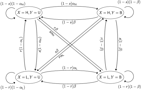
Figure 5: Transition diagram for a 2-state channel ($Y=\mathsf{U}$, unbound receptor; $Y=\mathsf{B}$, bound receptor) driven by a 2-state input Markov process ($X=\mathsf{L}$, low concentration of signaling molecule; $X=\mathsf{H}$, high concentration of signaling molecule). Probability per time step of $X_{k}=\mathsf{L}$ to $X_{k+1}=\mathsf{H}$ transition is $0<r\leq 1$. Probability per time step of $X_{k}=\mathsf{H}$ to $X_{k+1}=\mathsf{L}$ transition is $0<s\leq 1$. Probability per time step of $Y_{k}=\mathsf{U}$ to $Y_{k+1}=\mathsf{B}$ transition is $\alpha_{\mathsf{L}}$ when $X_{k}=\mathsf{L}$, and is $\alpha_{\mathsf{H}}$ when $X_{k}=\mathsf{H}$; these probabilities satisfy the strictly-ordered condition (Def. 1). Probability per time step of $Y_{k}=\mathsf{B}$ to $Y_{k+1}=\mathsf{U}$ is $0<\beta<1$, regardless of $X_{k}$. Compare Equation (90).

The input $X^{n}$ has a unique stationary distribution if $0<r,s<1$. The chain $Z^{n}$ has a stationary distribution if $X^{n}$ has a stationary distribution, and the parameters are strictly ordered. (These conditions are sufficient, but not necessary.) The steady-state distribution on $X$ is given by

$$p_{\mathsf{L}}=p_{X}(\mathsf{L})=\frac{s}{r+s},\hskip 28.45274ptp_{\mathsf{H}}=p_{X}(\mathsf{H})=\frac{r}{r+s}.$$ (91)

The stationary distribution of $Z$ is given by the (normalized) eigenvector of $\mathbf{P}_{Z}$ with unit eigenvalue. This is given by $[p_{X,Y}(\mathsf{L},\mathsf{U}),p_{X,Y}(\mathsf{L},\mathsf{B}),p_{X,Y}(\mathsf{H},\mathsf{U}),p_{X,Y}(\mathsf{H},\mathsf{B})]$, where

$$p_{X,Y}(\mathsf{L},\mathsf{U})=$$

$$\frac{1}{K}\left(\beta s(-r-s+\alpha_{\mathsf{H}}(r+s-1)+\beta(r+s-1))\right)$$

$$p_{X,Y}(\mathsf{L},\mathsf{B})=$$

$$\frac{1}{K}\left(s(\alpha_{\mathsf{H}}(\alpha_{\mathsf{L}}(r+s-1)-r)+\alpha_{\mathsf{L}}(\beta(r+s-1)-s))\right)$$

$$p_{X,Y}(\mathsf{H},\mathsf{U})=$$

$$\frac{1}{K}\left(\beta r(-r-s+\alpha_{\mathsf{L}}(r+s-1)+\beta(r+s-1))\right)$$

$$p_{X,Y}(\mathsf{H},\mathsf{B})=$$

$$\frac{1}{K}\left(r(\alpha_{\mathsf{H}}(-r+\alpha_{\mathsf{L}}(r+s-1)+\beta(r+s-1))-\alpha_{\mathsf{L}}s)\right),$$

where $K$ is the normalization constant, to ensure the probabilities sum to 1. The expressions (III-A-III-A) may be simplified by introducing the notation

$$\bar{\alpha} = \frac{r\alpha_{\mathsf{H}}+s\alpha_{\mathsf{L}}}{r+s}$$ (96)

$$\lambda = 1-r-s$$ (97)

$$\mu = \frac{\lambda}{1-\lambda}.$$ (98)

The quantity $\bar{\alpha}$ is the mean value of $\alpha$ under the equilibrium distribution for $X$ (cf. (18) for IID inputs); $\lambda$ is the second eigenvalue of the matrix $\mathbf{P}_{X}$; and $0\leq\mu<\infty$ is a monotonically increasing function of $\lambda$. With this notation, the stationary distribution of the joint process satisfies

$$p_{X,Y}(\mathsf{L},\mathsf{U}) = \frac{1}{K}\beta s(1+(\alpha_{\mathsf{H}}+\beta)\mu)$$ (99)

$$p_{X,Y}(\mathsf{L},\mathsf{B}) = \frac{1}{K}s(\bar{\alpha}+\alpha_{\mathsf{L}}(\alpha_{\mathsf{H}}+\beta)\mu)$$ (100)

$$p_{X,Y}(\mathsf{H},\mathsf{U}) = \frac{1}{K}\beta r(1+(\alpha_{\mathsf{L}}+\beta)\mu)$$ (101)

$$p_{X,Y}(\mathsf{H},\mathsf{B}) = \frac{1}{K}r(\bar{\alpha}+\alpha_{\mathsf{H}}(\alpha_{\mathsf{L}}+\beta)\mu),$$ (102)

with normalization constant

$$K=\lambda(\alpha_{\mathsf{L}}+\beta)(\alpha_{\mathsf{H}}+\beta)+(r+s)(\bar{\alpha}+\beta).$$ (103)

From $p_{X,Y}(X,Y)$ one may obtain the stationary marginal distribution $p_{Y}(y)$. Define

$$\Delta=\frac{s-r}{s+r}$$ (104)

to represent the relative difference in probabilities between the low-to-high and high-to-low transitions. Then

$$p_{Y}(\mathsf{U}) = \left(1+\mu(\bar{\alpha}+\beta+\Delta(\alpha_{\mathsf{H}}-\alpha_{\mathsf{L}}))\right)/K^{\prime}$$ (105)

$$p_{Y}(\mathsf{B}) = (\bar{\alpha}+\mu(\bar{\alpha}\beta+\alpha_{\mathsf{H}}\alpha_{\mathsf{L}}))/K^{\prime},$$ (106)

with normalization constant

$$K^{\prime}=1+\bar{\alpha}+\mu(\bar{\alpha}+\bar{\alpha}\beta+\beta+\alpha_{\mathsf{H}}\alpha_{\mathsf{L}}+\Delta(\alpha_{\mathsf{H}}-\alpha_{\mathsf{L}})).$$ (107)

III-B Capacity estimates for Markov inputs

To estimate capacity for Markov inputs, we need the entropy rates for $X$, $Y$, and $Z$. Since $X$ and $Z$ are stationary Markov processes, their entropy rates are available in closed form. The entropy rate of $X$ is given as a function of $r$ and $s$ by

$$\mathcal{H}(X) =\lim_{n\rightarrow\infty}\frac{1}{n}H(X^{n})$$ (108)

$$=H(X_{i}\>|\>X_{i-1})$$ (109)

$$=p_{\mathsf{L}}\left(r\log\frac{1}{r}+(1-r)\log\frac{1}{1-r}\right)$$ (110)

$$\>\>+p_{\mathsf{H}}\left(s\log\frac{1}{s}+(1-s)\log\frac{1}{1-s}\right).$$

The joint entropy rate $\mathcal{H}(Z)=\mathcal{H}(X,Y)$ can be calculated directly from (99)-(103). Let

$$\pi_{xy}=p_{X,Y}(x,y)$$ (111)

denote the stationary density of the Markov process, i.e. the four terms given in (99)-(102). Denote the joint transition probabilities from the matrix $\mathbf{P}_{Z}$ as

$$T_{xy\rightarrow x^{\prime}y^{\prime}} =p_{X_{i},Y_{i}|X_{i-1},Y_{i-1}}(x^{\prime},y^{\prime}\>|\>x,y)$$ (112)

$$=p_{Y_{i}|X_{i-1},Y_{i-1}}(y^{\prime}\>|\>x,y)p_{X_{i}|X_{i-1}}(x^{\prime}\>|\>x).$$ (113)

Further let

$$\phi(p)=-p\log p.$$ (114)

Then the joint entropy rate is

$$\mathcal{H}(X,Y)=\sum_{x=\mathsf{L}}^{\mathsf{H}}\sum_{y=\mathsf{U}}^{\mathsf{B}}\pi_{xy}\left(\sum_{x^{\prime}=\mathsf{L}}^{\mathsf{H}}\sum_{y^{\prime}=\mathsf{U}}^{\mathsf{B}}\phi\left(T_{xy\rightarrow x^{\prime}y^{\prime}}\right)\right).$$ (115)

However, the output process $Y$ is not a Markov process in general, and its entropy rate is not available in closed form. To bound the entropy rate of $Y$, we use the fact that this rate $\mathcal{H}(Y)$ is bounded above and below by entropies conditioned on a finite number of previous channel states. From standard inequalities ([75], Theorem 4.4.1) we have, for each $n$,

$$H(Y_{n}|X_{0},Y_{0},\cdots,Y_{n-1})$$

$$\leq\mathcal{H}(Y)\leq H(Y_{n}|Y_{0},\cdots,Y_{n-1})$$ (116)

and

$$\lim_{n\to\infty}H(Y_{n}|X_{0},Y_{0},\cdots,Y_{n-1})$$

$$=\mathcal{H}(Y)=\lim_{n\to\infty}H(Y_{n}|Y_{0},\cdots,Y_{n-1}).$$ (117)

Using the inequalities (116), we have

$$\mathcal{I}(X;Y) =\mathcal{H}(X)+\mathcal{H}(Y)-\mathcal{H}(X,Y)$$ (118)

$$\leq\mathcal{H}(X)-\mathcal{H}(X,Y)+H(Y_{n}|Y_{0},\cdots,Y_{n-1})$$ (119)

$$=:\mathcal{I}_{n}^{+}(X;Y)$$ (120)

and

$$\mathcal{I}(X;Y) \geq\mathcal{H}(X)-\mathcal{H}(X,Y)+H(Y_{n}|X_{0},Y_{0},\cdots,Y_{n-1})$$ (121)

$$=:\mathcal{I}_{n}^{-}(X;Y).$$ (122)

The required bounds on $\mathcal{H}(Y)$ are derived below.

III-B1 Upper Bounds on $\mathcal{H}(Y)$ and $\mathcal{I}(X;Y)$

First consider the one-step conditional entropy of the $Y$ sequence,

$$H(Y_{1}|Y_{0})$$ (123)

$$= \sum_{y_{0}}p_{Y}(y_{0})\mathscr{H}\left(p_{Y_{1}|Y_{0}}(\mathsf{B}\>|\>y_{0})\right)$$

$$= \sum_{y_{0}}p_{Y}(y_{0})\mathscr{H}\left(\sum_{x_{0},x_{1}}\frac{\pi_{x_{0}y_{0}}T_{x_{0}y_{0}\rightarrow x_{1}\mathsf{B}}}{\pi_{\mathsf{L}y_{0}}+\pi_{\mathsf{H}y_{0}}}\right),$$ (124)

where $\mathscr{H}$ is the binary entropy function, and $\pi_{xy}$ and $T_{x_{0}y_{0}\rightarrow x_{1}\mathsf{B}}$ are the steady-state probability (resp. transition probability) of the $(X,Y)$ Markov chain, defined in (111) (resp. (113)). At the same time, the mutual information rate is bounded above by the entropy rate of the input (110). Thus, from (110), (115), and (124), the first upper bound $\mathcal{I}_{1}^{+}(X;Y)$ is given by

$$\mathcal{I}_{1}^{+}(X;Y)=$$

$$p_{\mathsf{L}}\left(r\log\frac{1}{r}+(1-r)\log\frac{1}{1-r}\right)$$

$$+p_{\mathsf{H}}\left(s\log\frac{1}{s}+(1-s)\log\frac{1}{1-s}\right)$$

$$+\left\{\left[\>-\>\sum_{x=\mathsf{L}}^{\mathsf{H}}\sum_{y=\mathsf{U}}^{\mathsf{B}}\pi_{xy}\left(\sum_{x^{\prime}=\mathsf{L}}^{\mathsf{H}}\sum_{y^{\prime}=\mathsf{U}}^{\mathsf{B}}\phi\left(T_{xy\rightarrow x^{\prime}y^{\prime}}\right)\right)\right.\right.$$

$$\left.\left.\>+\>\sum_{y_{0}}p_{Y}(y_{0})\mathscr{H}\left(\sum_{x_{0},x_{1}}\frac{T_{x_{0}y_{0}\rightarrow x_{1}\mathsf{B}}\pi_{x_{0}y_{0}}}{\pi_{\mathsf{L}y_{0}}+\pi_{\mathsf{H}y_{0}}}\right)\right]\wedge\>0\right\},$$ (125)

where $\{A\wedge B\}$ represents the lesser of $A$ and $B$. The bound $\mathcal{I}_{1}^{+}(X;Y)$ is illustrated in Figure 6.

Figure 6: Mutual information upper bound given by (125), for $\alpha_{\mathsf{L}}=0.1,\alpha_{\mathsf{H}}=0.9,\beta=0.5$. Horizontal axis: $r$; vertical axis: $s$.

Next consider the two-step entropy, $H(Y_{2}|Y_{0},Y_{1})$. We calculate this entropy explicitly as follows:

$$H(Y_{2}|Y_{0},Y_{1})=\sum_{y_{0},y_{1}}p_{Y_{0},Y_{1}}(y_{0},y_{1})\mathscr{H}\left(p_{Y_{2}|Y_{0},Y_{1}}(\mathsf{B}\>|\>y_{0},y_{1})\right),$$ (126)

where

$$p_{Y_{0},Y_{1}}(y_{0},y_{1}) =\sum_{x_{0},x_{1}}\pi_{x_{0}y_{0}}T_{x_{0}y_{0}\to x_{1}y_{1}}$$ (127)

$$p_{Y_{2}|Y_{0},Y_{1}}(\mathsf{B}\>|\>y_{0},y_{1}) =\sum_{x_{2}}p_{X_{2},Y_{2}|Y_{0},Y_{1}}(x_{2},\mathsf{B}\>|\>y_{0},y_{1})$$ (128)

and, writing $X_{0}^{n}$ for $(X_{0},\cdots,X_{n})$,

$$p_{X_{2},Y_{2}|Y_{0},Y_{1}}(x_{2},\mathsf{B}\>|\>y_{0},y_{1})$$

$$=\sum_{x_{0},x_{1}}p_{X_{0}^{2},Y_{2}|Y_{0},Y_{1}}(x_{0}^{2},\mathsf{B}\>|\>y_{0},y_{1})$$ (129)

$$=\sum_{x_{0},x_{1}}\left(\frac{T_{x_{1}y_{1}\to x_{2}\mathsf{B}}p_{X_{0},Y_{0},X_{1},Y_{1}}(x_{0},y_{0},x_{1},y_{1})}{\sum_{x_{0},x_{1}}p_{X_{0},Y_{0},X_{1},Y_{1}}(x_{0},y_{0},x_{1},y_{1})}\right)$$ (130)

$$=\sum_{x_{0},x_{1}}\left(\frac{T_{x_{1}y_{1}\to x_{2}\mathsf{B}}T_{x_{0}y_{0}\rightarrow x_{1}y_{1}}\pi_{x_{0}y_{0}}}{\sum_{x_{0},x_{1}}T_{x_{0}y_{0}\rightarrow x_{1}y_{1}}\pi_{x_{0}y_{0}}}\right).$$ (131)

In general, the $n^{\text{th}}$ upper bound of this form is obtained from the $n$-step upper bound of the entropy rate of the channel state. Writing $Y_{0}^{n-1}$ for $(Y_{0},\cdots,Y_{n-1})\in\{\mathsf{U},\mathsf{B}\}^{n}$, the $n$-step upper bound is given by a sum involving $2^{n}$ terms

$$\mathcal{H}^{+}_{n} :=H(Y_{n}|Y_{0}^{n-1})$$ (132)

$$=\sum_{y_{0}^{n-1}\in\{\mathsf{U},\mathsf{B}\}^{n}}p_{Y_{0}^{n-1}}(y_{0}^{n-1})\mathscr{H}(p_{Y_{n}|Y_{0}^{n-1}}(\mathsf{B}\>|\>y_{0}^{n-1})).$$ (133)

In appendix -E we briefly show how to use the sum-product algorithm to calculate the general $n$-step bound. Figure 7 illustrates the convergence of the sequence of upper bounds $\mathcal{H}_{n}^{+}$ with a similar sequence of lower bounds (next section) for $n=2,3,4,5$.

III-B2 Lower Bounds on $\mathcal{H}(Y)$ and $\mathcal{I}(X;Y)$

In a similar fashion, we can formulate a lower bound on $\mathcal{H}(Y)$ involving $n$ prior states of $Y$ and the initial state of $X$, namely

$$\mathcal{H}^{-}_{n} :=H(Y_{n}|X_{0},Y_{0}^{n-1})$$ (134)

$$=\sum_{x_{0}\in\{\mathsf{L},\mathsf{H}\}}\sum_{y_{0}^{n-1}\in\{\mathsf{U},\mathsf{B}\}^{n}}p_{X_{0},Y_{0}^{n-1}}(x_{0},y_{0}^{n-1})$$

$$\>\>\cdot\mathscr{H}(p_{Y_{n}|X_{0},Y_{0}^{n-1}}(\mathsf{B}\>|\>x_{0},y_{0}^{n-1})).$$ (135)

Moreover, we also have the trivial lower bound on the mutual information rate $\mathcal{I}(X;Y)\geq 0$.

Again, appendix -E briefly shows how to perform this calculation using the sum-product algorithm. Figure 7 illustrates the convergence of $\mathcal{H}^{\pm}_{n}$ in the interior of the region $0<r,s<1$, for $n=2,3,4,5$.

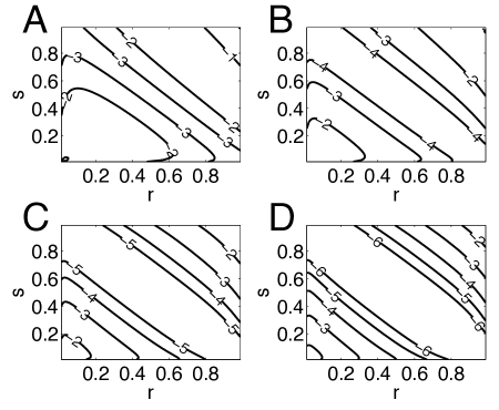
Figure 7: Difference between upper and lower bounds for the mutual information rate $\mathcal{I}(X;Y)$ of the 2-state Markov channel, as a function of switching parameters $0<r<1$ and $0<s<1$. The upper and lower bounds are given by (119) and (122), respectively. Each panel shows $\log_{10}(\mathcal{I}^{+}_{n}-\mathcal{I}^{-}_{n})$ for $n=2$ (panel A), $n=3$ (panel B), $n=4$ (panel C), $n=5$ (panel D). Parameter values are $\alpha_{\mathsf{L}}=0.1,\beta=0.5,\alpha_{\mathsf{H}}=0.9$. Each increase in the depth of conditioning decreases the gap between the upper and lower bounds by roughly an order of magnitude.

The upper and lower bounds obtained by conditioning $Y$ to a depth of five steps constrains the mutual information to within less than 1% for input switching rates satisfying $|r+s-1|\lesssim 0.9$, or roughly all but 1% of the $(r,s)$ plane, for the parameters ($\alpha_{\mathsf{L}}=0.1,\beta=0.5,\alpha_{\mathsf{H}}=0.9$) illustrated in Fig. 7. (Elsewhere, the bounds can be obtained to greater depth using the same procedure.) We confirmed this result using Monte Carlo sampling to obtain empirical mutual information rates.

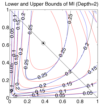
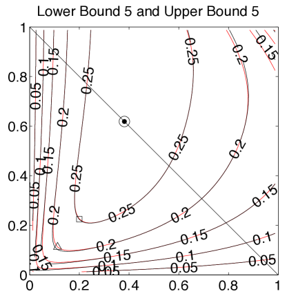
Figure 8: Mutual information of the two-state channel driven by a two-state Markov input process. The channel parameters are $\alpha_{\mathsf{L}}=0.1,\beta=0.5,\alpha_{\mathsf{H}}=0.9$. The input switching rates are $r$ (low-to-high) and $s$ (high-to-low). Top: Three sets of curves show the upper bound $\mathcal{I}_{2}^{+}(X;Y)$ (black), lower bound $\mathcal{I}_{2}^{-}(X;Y)$ (red), and Monte Carlo estimate (blue). The diagonal line represents $r+s=1$, along which the Markov input process reduces to IID; the capacity-achieving input distribution occurs along this line. Contour labels refer to the upper bound (black curve). The UB, LB and MC curves coincide when $r+s=1$. Bottom: Two sets of curves show the upper bound (black curves) and lower bound (red curves) $\mathcal{I}_{5}^{\pm}(X;Y)$, which are indistinguishable over most of the $(r,s)$ plane. Horizontal axis: $r$; vertical axis: $s$. Circled dot indicates capacity-achieving IID input switching rates $r_{\text{opt}}\approx 0.381,s_{\text{opt}}\approx 0.619$; at this point $\mathcal{I}_{5}^{\pm}(X;Y)\approx 0.279$. Square: $(r,s)\approx(0.200,0.225)$. Triangle: $(r,s)\approx(0.112,0.112)$. See text for details.

Figure 8, which shows the mutual information surface for parameters $\alpha_{\mathsf{L}}=0.1,\beta=0,5,\alpha_{\mathsf{H}}=0.9$, as a function of low-to-high switching rate $r$, and high-to-low switching rate $s$, provides several insights. First, the upper panel shows reasonable agreement between the upper bound, the lower bound, and direct Monte Carlo sampling, even when the UB and LB are only calculated to a depth of two levels of conditioning (the top panel plots $\mathcal{I}_{2}^{\pm}(X;Y)$ together with the Monte Carlo estimate). Second, consistent with Figure 7, conditioning five steps deep gives indistinguishable upper and lower bounds for all but a small portion of the $(r,s)$ plane. Third, the channel can endure a significant departure from the idealized IID input case with only a modest loss of efficiency. In the lower panel the $\text{MI}=0.25$ contour represents a roughly 10% decrement in the mutual information rate relative to the capacity ($\approx 0.279$ bits per time step, for these parameters). This contour extends to $r+s$ values as low as $r+s\approx 0.425$. Finally, by introducing memory into the channel (deviating from the line $r+s=1$) we gradually change the optimal strategy for deploying high- versus low-concentration input signals. To see this, note that the closest point to the origin along the $\text{MI}=0.25$ contour is $(r_{\square},s_{\square})\approx(0.200,0.225)$, marked $\square$ on the bottom panel of Figure 8. When the input is IID, the optimal low- versus high-input frequency is biased towards low-concentration inputs ($s_{\text{opt}}/r_{\text{opt}}\approx 0.619/0.381\approx 1.62$). As the sum of the switching rates decreases, this bias is gradually reduced; for low switching rates (close to the origin of the $(r,s)$ plane) the optimal ratio approaches unity. For example, at the point $\square$ the low-input–frequency to high-input–frequency ratio is $s_{\square}/r_{\square}\approx.225/.200\approx 1.12$. At the next contour ($\mathcal{I}_{5}^{\pm}(X;Y)\approx 0.20$) the closest point to the origin, marked $\triangle$, is $(r_{\triangle},s_{\triangle})\approx(0.112,0.112)$. At this point the low-input–frequency to high-input–frequency ratio is approximately unity. Our analysis of the two-state discrete time BIND channel, with input constrained to a two-state Markov process, suggests that we could expect to see different signaling strategies employed in specific biological channels, depending on the persistence times of diffusion-mediated signals in those channels.

IV Continuous-time limits of the discrete time channel

The BIND channel arises from an underlying physical system – ligand molecules binding to a receptor protein – that operates in continuous rather than discrete time. The per timestep transition probabilities $\alpha_{\mathsf{L}/\mathsf{H}}$ and $\beta$ derive from continuous time transition rates $k_{+}$ and $k_{-}$ in the sense that $\alpha_{\mathsf{L}/\mathsf{H}}=k_{+}c_{\mathsf{L}/\mathsf{H}}\,\Delta t+o(\Delta t)$ and $\beta=k_{-}\,\Delta t+o(\Delta t)$ (cf. §I-B). Rigorous analysis of point process channels in continuous time requires additional probability theoretic techniques beyond the scope of the present paper (for results in this direction, see[69, 76, 77, 78]). Nevertheless it is of interest to study how the mutual information and capacity of the discrete time BIND channel behave in the limit of small time steps.

In this section we therefore consider the capacity of the discrete time BIND channel in two limiting cases. In §IV-A we evaluate the limiting behavior of the discrete time mutual information rate in the limit of short time steps, and its supremum with respect to parameters. While this approach does not provide a rigorous proof of a continuous-time capacity formula, the limiting form of the mutual information per time step takes an intuitively appealing form, namely the product of the mutual information rate of a counting process when the channel is in the receptive or unbound state, multiplied by the fraction of time it is in that state under stationary input conditions. In §IV-B we again consider the short time-step limit of the mutual information, but do so while fixing the per time-step release probability to be unity. Although again not a rigorous proof of capacity, in this case it is interesting to note that the continuous time channel without an insensitive or bound state gives the same limiting mutual information rate and capacity expression as Kabanov’s Poisson channel (Wyner 1988a, Wyner 1988b). This limit provides an important consistency check on the discrete time BIND model, and indicates its connection to existing point process models.

IV-A Derivation of a capacity expression for the 2-state signal transduction channel

We start with the expression for the discrete time mutual information rate (82). Assuming the input distribution is IID, the mutual information per discrete time step is given by

$$I(X;Y)=\frac{\mathscr{H}(\alpha_{\mathsf{H}}p_{\mathsf{H}}+\alpha_{\mathsf{L}}p_{\mathsf{L}})-p_{\mathsf{H}}\mathscr{H}(\alpha_{\mathsf{H}})-p_{\mathsf{L}}\mathscr{H}(\alpha_{\mathsf{L}})}{1+(p_{\mathsf{H}}\alpha_{\mathsf{H}}+p_{\mathsf{L}}\alpha_{\mathsf{L}})/\beta},$$ (136)

where

$$\mathscr{H}(p)=-p\log p-(1-p)\log(1-p).$$ (137)

The IID capacity is obtained by maximizing over the set $p_{\mathsf{H}}\in[0,1]$ with $p_{\mathsf{L}}=1-p_{\mathsf{H}}$. For convenience, we use $x$ to represent $p_{\mathsf{H}}$ in the rest of this section.

The discrete time channel model assumes that the probability of transition per time step is $\alpha_{\mathsf{H}},\alpha_{\mathsf{L}},$ or $\beta$, depending on the state of the input and the state of the channel. The IID input approximation assumes the input can flicker back and forth arbitrarily fast, so that successive time steps are uncorrelated. For the following calculation, we will assume that the input can remain IID even in the limit of vanishing time step. To represent discretization with an arbitrary time step, we set

$$\alpha^{*}_{\mathsf{H}} = \epsilon\alpha_{\mathsf{H}}$$

$$\alpha^{*}_{\mathsf{L}} = \epsilon\alpha_{\mathsf{L}}$$

$$\beta^{*} = \epsilon\beta$$

where $\epsilon>0$ is the size of the time step. The case $\epsilon=1$ corresponds to the discrete time model considered in §II. The fixed constants $\alpha_{\mathsf{H}/\mathsf{L}}$ and $\beta$ now represent transition rates per unit time, rather than probabilities per time step.

Figure 9 shows the per-time-step mutual information, as a function of $0\leq x\leq 1$, for $\alpha^{*}_{\mathsf{L}}=0.1\epsilon$, $\alpha^{*}_{\mathsf{H}}=0.9\epsilon$, and $\beta^{*}=0.5\epsilon$, for $\epsilon$ ranging from 1 to $10^{-4}$.

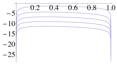
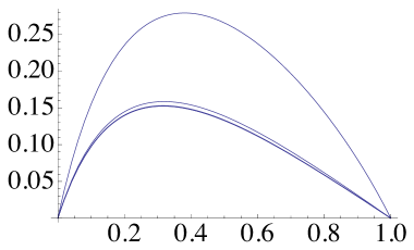
Figure 9: Convergence of mutual information rate as $\epsilon\to 0$. Left: Log of the mutual information per time step, $\log(I(X;Y))$, plotted as a function of $x\in[0,1]$, for $\alpha_{\mathsf{L}}^{*}=0.1\epsilon$, $\alpha_{\mathsf{H}}^{*}=0.9\epsilon$, and $\beta^{*}=0.5\epsilon$. The curves stacked from top to bottom have $\epsilon=1,0.1,0.01,0.001$ and $0.0001$, respectively. Right: Mutual information rate, $I/\epsilon$, for the same parameters. The top curve has $\epsilon=1$; the next has $\epsilon=0.1$; the rest are indistinguishable. The curves suggest that as $\epsilon\to 0$, the mutual information rate $I/\epsilon$ converges to a finite quantity, and that the location of the maximum converges to a given value $x_{\text{opt}}$ as well.

The curves suggest that, as expected, the optimal value of $x$ lies in the interior of the interval $(0,1)$. Moreover, the optimal value appears to converge to a given value $x_{\text{opt}}$ as $\epsilon\to 0$, distinct from the optimal value when $\epsilon=1$.

We define the mutual information rate for a given $\epsilon>0$, $\mathcal{I}_{\epsilon}$, to be $I/\epsilon$, and we study how this quantity scales as $\epsilon\to 0^{+}$. In the remainder of this section we do the following:

1. We study the information rate $\mathcal{I}_{\epsilon}(x)$ for small $\epsilon$ and show that it has a unique maximum in the interior of the interval $0\leq x\leq 1$, where $x=p_{\mathsf{H}}$ is the probability that the input signal is in the “high” concentration state.

2. By taking the limit as $\epsilon\to 0^{+}$, and optimizing over $x$, we obtain an expression for the capacity of the discrete time channel in the continuous time limit, as a function of the binding and unbinding rates $\alpha_{\mathsf{H}}$, $\alpha_{\mathsf{L}}$, and $\beta$.

In the following section §IV-B, we further show that by taking the limit of the capacity for the continuous time channel, as the unbinding rate $\beta\to\infty$, we recover Kabanov’s expression for the capacity for the Poisson channel.

IV-A1 Critical point of the information rate $\mathcal{I}_{\epsilon}$ for small $\epsilon>0$

First we study the behavior of the optimal value of $x$ in the limit of small $\epsilon$. Assuming an interior maximum for $I$, we set the derivative of the RHS of Equation (219) equal to zero to obtain the necessary and sufficient condition in equation (138).

$$0 = -\alpha_{\mathsf{H}}\beta\epsilon\log\left(\frac{1}{-\alpha_{\mathsf{H}}x\epsilon+\alpha_{\mathsf{L}}(x-1)\epsilon+1}\right)+\alpha_{\mathsf{L}}\beta\epsilon\log\left(\frac{1}{-\alpha_{\mathsf{H}}x\epsilon+\alpha_{\mathsf{L}}(x-1)\epsilon+1}\right)$$ (138)

$$+\beta\epsilon(\alpha_{\mathsf{H}}-\alpha_{\mathsf{L}})\log\left(\frac{1}{\alpha_{\mathsf{H}}x\epsilon-\alpha_{\mathsf{L}}x\epsilon+\alpha_{\mathsf{L}}\epsilon}\right)-\alpha_{\mathsf{H}}\epsilon(\alpha_{\mathsf{L}}+\beta)\log\left(\frac{1}{\alpha_{\mathsf{H}}\epsilon}\right)$$

$$+\alpha_{\mathsf{L}}\epsilon(\alpha_{\mathsf{H}}+\beta)\log\left(\frac{1}{\alpha_{\mathsf{L}}\epsilon}\right)-\alpha_{\mathsf{H}}\log\left(\frac{1}{-\alpha_{\mathsf{H}}x\epsilon+\alpha_{\mathsf{L}}(x-1)\epsilon+1}\right)$$

$$+\alpha_{\mathsf{L}}\log\left(\frac{1}{-\alpha_{\mathsf{H}}x\epsilon+\alpha_{\mathsf{L}}(x-1)\epsilon+1}\right)-\alpha_{\mathsf{L}}\log\left(\frac{1}{1-\alpha_{\mathsf{H}}\epsilon}\right)+\alpha_{\mathsf{H}}\alpha_{\mathsf{L}}\epsilon\log\left(\frac{1}{1-\alpha_{\mathsf{H}}\epsilon}\right)$$

$$+\alpha_{\mathsf{H}}\log\left(\frac{1}{1-\alpha_{\mathsf{L}}\epsilon}\right)-\alpha_{\mathsf{H}}\alpha_{\mathsf{L}}\epsilon\log\left(\frac{1}{1-\alpha_{\mathsf{L}}\epsilon}\right)-\beta\log\left(\frac{1}{1-\alpha_{\mathsf{H}}\epsilon}\right)$$

$$+\alpha_{\mathsf{H}}\beta\epsilon\log\left(\frac{1}{1-\alpha_{\mathsf{H}}\epsilon}\right)+\beta\log\left(\frac{1}{1-\alpha_{\mathsf{L}}\epsilon}\right)-\alpha_{\mathsf{L}}\beta\epsilon\log\left(\frac{1}{1-\alpha_{\mathsf{L}}\epsilon}\right).$$

In Appendix -F we show that this condition leads to an interior maximum at a unique value of $x$ as $\epsilon\to 0$.

IV-A2 Implicit expression for $x_{\text{opt}}$ in the limit $\epsilon\to 0$, and an expression for the limiting capacity of the discrete time channel in the small $\epsilon$ limit

Define the continuous time information rate, as a function of the fraction of time the input is in the higher state ($x=p_{\mathsf{H}}$), as

$$\mathcal{I} =\lim_{\epsilon\to 0^{+}}\left(\frac{1}{\epsilon}I(X;Y)\right).$$ (139)

with $I(X;Y)$ given in (136). From the preceding section, we know this expression converges to a finite value, and moreover $\mathcal{I}$ has a unique maximum in the range $0\leq x\leq 1$. Let $x_{\text{opt}}$ denote the optimal value of the high-input probability. It is straightforward to show that

$$\mathcal{I}(x)=$$ (140)

$$-\left(\frac{\beta}{\beta+\bar{\alpha}}\right)\Big{(}\bar{\alpha}\log(\bar{\alpha})-(x\alpha_{\mathsf{H}}\log\alpha_{\mathsf{H}}+(1-x)\alpha_{\mathsf{L}}\log\alpha_{\mathsf{L}})\Big{)}$$

where, as above, $\bar{\alpha}(x)=x\alpha_{\mathsf{H}}+(1-x)\alpha_{\mathsf{L}}$ is the average value of $\alpha$ given $x$. Thus the mutual information rate is given by the product of the fraction of time the channel is in the receptive state,

$$f(x)\equiv\left(\frac{\beta}{\beta+\bar{\alpha}(x)}\right)$$

and the mutual information rate conditional on the channel being in the receptive state,

$$g(x)\equiv-(\bar{\alpha}(x)\log\bar{\alpha}(x)-(x\alpha_{\mathsf{H}}\log\alpha_{\mathsf{H}}+(1-x)\alpha_{\mathsf{L}}\log\alpha_{\mathsf{L}})).$$

Although the optimal value of the high input probability $x$ is not available explicitly, we can obtain a useful implicit expression for the small $\epsilon$ limiting capacity of the discrete time channel. Setting $\mathcal{I}^{\prime}=f^{\prime}g+fg^{\prime}=0$, and noting that $f^{\prime}<0,$ we have $g(x_{\text{opt}})=f(x_{\text{opt}})g^{\prime}(x_{\text{opt}})/f^{\prime}(x_{\text{opt}})$, from which

$$\mathcal{I}(x_{\text{opt}})$$ (142)

$$= \frac{g^{\prime}(x_{\text{opt}})}{f^{\prime}(x_{\text{opt}})}f(x_{\text{opt}})^{2}$$

$$= \left(\frac{\beta}{\alpha_{\mathsf{H}}-\alpha_{\mathsf{L}}}\right)\Big{(}\alpha_{\mathsf{H}}\log\alpha_{\mathsf{H}}-\alpha_{\mathsf{L}}\log\alpha_{\mathsf{L}}$$

$$-\>(\alpha_{\mathsf{H}}-\alpha_{\mathsf{L}})(1+\log\bar{\alpha}(x_{\text{opt}}))\Big{)}.$$

In the continuous time setting, we have an ambiguity associated with the choice of the time unit. Provided the low binding rate is not identically zero, we can choose time units with respect to which the low binding rate $\alpha_{\mathsf{L}}\equiv 1$. Let $\alpha_{\mathsf{H}}=1+c$ in the same units. Thus, from (142), the capacity is given by

$$\mathcal{I}(x_{\text{opt}})=\beta\left(\frac{1+c}{c}\log(1+c)-1-\log(1+x_{\text{opt}}c)\right).$$ (143)

Although $x_{\text{opt}}$ is not known explicitly, it lies in the interior of the unit interval, so we have the upper and lower bounds

$$\beta\left(\frac{1+c}{c}\log(1+c)-1-\log(1+c)\right)$$

$$\leq\mathcal{I}(x_{\text{opt}})\leq$$ (144)

$$\beta\left(\frac{1+c}{c}\log(1+c)-1\right).$$

Kabanov obtained the capacity of the Poisson channel with signal intensity bounded above by a constant $c$, and unit background intensity. The “high” and “low” rates of the incoming process (combining signal and noise) were $1+c$ and $1$, respectively. In the limit as the unbinding rate grows without bound, we expect that our channel should be equivalent to Kabanov’s Poisson channel. Note that because the optimal sending input distribution depends on the channel parameters, including $\beta$, the expression (143) does not necessarily diverge as $\beta\to\infty$. In the next section we recover Kabanov’s capacity formula in this limit.

IV-B Reduction of the 2-State Signal-Transduction Channel to Kabanov’s Poisson Channel

In the introduction, we discussed Kabanov’s capacity [69], which assumes $k_{-}\rightarrow\infty$ (i.e., the $\mathsf{B}\rightarrow\mathsf{U}$ transition is immediate and instantaneous). In this section, we come full circle by showing that Kabanov’s capacity formula emerges when we take the limit as $\epsilon\rightarrow 0$ and $k_{-}\rightarrow\infty$ of the discrete time BIND channel.

Let us suppose that with a discrete time step $\epsilon$, we may set the unbinding rate $k_{-}=1/\epsilon$, so that the unbinding probability is fixed at $\beta=\epsilon k_{-}=1$; thus, $k_{-}$ is set to the highest possible rate such that $\beta$ is a valid probability. Further, recall that $\alpha_{\mathsf{H}}=\epsilon k_{+}c_{\mathsf{H}}$ and $\alpha_{\mathsf{L}}=\epsilon k_{+}c_{\mathsf{L}}$, and let $\bar{k}_{x}=xk_{+}c_{\mathsf{H}}+(1-x)k_{+}c_{\mathsf{L}}$ represent the average binding rate.

Suppose $\epsilon\rightarrow 0$; setting $k_{-}=1/\epsilon$, this means $k_{-}\rightarrow\infty$. The continuous time channel capacity is still bounded, provided the low sending rate $\alpha_{\mathsf{L}}>0$, so we can write

$$\mathcal{I}_{\epsilon}(x)=$$ (145)

$$\frac{1}{\epsilon}\left(\frac{1}{1+\epsilon\bar{k}_{x}}\right)\Big{(}\mathscr{H}(\epsilon\bar{k}_{x})$$

$$\>\>-\>x\mathscr{H}(\epsilon k_{+}c_{\mathsf{H}})-(1-x)\mathscr{H}(\epsilon k_{+}c_{\mathsf{L}})\Big{)}$$

$$\lim_{\epsilon\to 0}\mathcal{I}_{\epsilon}(x)\equiv\mathcal{I}_{0}(x)$$ (146)

$$=xk_{+}c_{\mathsf{H}}\log k_{+}c_{\mathsf{H}}$$

$$\>\>+\>(1-x)k_{+}c_{\mathsf{L}}\log k_{+}c_{\mathsf{L}}-\bar{k}_{x}\log\bar{k}_{x}$$

$$\frac{d}{dx}\mathcal{I}_{0}(x)=$$ (147)

$$k_{+}c_{\mathsf{H}}\log k_{+}c_{\mathsf{H}}-k_{+}c_{\mathsf{L}}\log k_{+}c_{\mathsf{L}}$$

$$\>\>-\>(k_{+}c_{\mathsf{H}}-k_{+}c_{\mathsf{L}})(1+\log\bar{k}_{x})$$

and $\frac{d}{dx}\mathcal{I}_{0}(x)=0$ when

$$\log\bar{k}_{x}= \left(\frac{1}{k_{+}c_{\mathsf{H}}-k_{+}c_{\mathsf{L}}}\right)\cdot$$ (148)

$$\cdot\left(k_{+}c_{\mathsf{H}}\log\left(\frac{k_{+}c_{\mathsf{H}}}{e}\right)-k_{+}c_{\mathsf{L}}\log\left(\frac{k_{+}c_{\mathsf{L}}}{e}\right)\right).$$

Recall that $x_{\text{opt}}$ denotes the optimal probability of the high-concentration signal. Since $\bar{\alpha}=\alpha_{\mathsf{L}}+x_{\text{opt}}(\alpha_{\mathsf{H}}-\alpha_{\mathsf{L}})$, we have

$$x_{\text{opt}}=\frac{\bar{k}_{x}-k_{+}c_{\mathsf{L}}}{k_{+}c_{\mathsf{H}}-k_{+}c_{\mathsf{L}}}$$ (149)

and

$$(1-x_{\text{opt}})=\frac{k_{+}c_{\mathsf{H}}-\bar{k}_{x}}{k_{+}c_{\mathsf{H}}-k_{+}c_{\mathsf{L}}}.$$ (150)

Consequently the capacity, $\mathcal{I}_{0}^{*}=\mathcal{I}_{0}(x_{\text{opt}})$, reduces to

$$\mathcal{I}^{*}_{0} =\bar{k}_{x_{\text{opt}}}-\left(\frac{k_{+}c_{\mathsf{H}}k_{+}c_{\mathsf{L}}}{k_{+}c_{\mathsf{H}}-k_{+}c_{\mathsf{L}}}\right)\log\left(\frac{k_{+}c_{\mathsf{H}}}{k_{+}c_{\mathsf{L}}}\right)$$ (151)

$$=\exp\left[\left(\frac{1}{c_{\mathsf{H}}-c_{\mathsf{L}}}\right)\left(c_{\mathsf{H}}\log\left(\frac{k_{+}c_{\mathsf{H}}}{e}\right)-c_{\mathsf{L}}\log\left(\frac{k_{+}c_{\mathsf{L}}}{e}\right)\right)\right]$$

$$\>\>-\>\left(\frac{k_{+}c_{\mathsf{H}}c_{\mathsf{L}}}{c_{\mathsf{H}}-c_{\mathsf{L}}}\right)\log\left(\frac{c_{\mathsf{H}}}{c_{\mathsf{L}}}\right).$$ (152)

Now let $\lambda=k_{+}c_{\mathsf{L}}$ and $c=k_{+}c_{\mathsf{H}}-k_{+}c_{\mathsf{L}}$. Since $k_{-}\rightarrow\infty$, this corresponds to a Poisson channel, alternating between rates $\lambda$ and $\lambda+c$; these are Kabanov’s parameters. Substituting into the above equation,

$$\mathcal{I}_{o}^{*}(c,\lambda)$$

$$= \lambda+x_{\text{opt}}c-\left(\frac{\lambda(\lambda+c)}{c}\right)\log\left(\frac{\lambda+c}{\lambda}\right)$$

$$= \exp\left[\frac{\lambda+c}{c}\log\left(\frac{\lambda+c}{e}\right)-\frac{\lambda}{c}\log\left(\frac{\lambda}{e}\right)\right]$$

$$\>\>-\>\frac{\lambda}{c}(\lambda+c)\log\left(\frac{\lambda+c}{\lambda}\right)$$

$$= \exp\left[\left(1+\frac{\lambda}{c}\right)\log(\lambda+c)-\frac{\lambda}{c}\log\lambda-1\right]$$

$$\>\>-\>\lambda\left(1+\frac{\lambda}{c}\right)\log\left(1+\frac{c}{\lambda}\right)$$

$$= \exp\left[\log\left[\frac{(\lambda+c)^{(1+\lambda/c)}}{\lambda^{(\lambda/c)}e}\right]\right]$$

$$\>\>-\>\lambda\left(1+\frac{\lambda}{c}\right)\log\left(1+\frac{c}{\lambda}\right)$$

$$= \lambda\left[\frac{1}{e}\left(1+\frac{c}{\lambda}\right)^{(1+\lambda/c)}-\left(1+\frac{\lambda}{c}\right)\log\left(1+\frac{c}{\lambda}\right)\right].$$

Setting $\lambda=1$ in (LABEL:eq:davis-capacity) yields

$$\mathcal{I}_{o}^{*}(c,1) =\frac{1}{e}\left((c+1)^{1+c^{-1}}\right)-\left(1+\frac{1}{c}\right)\log(c+1)$$ (158)

$$=C_{\text{Kabanov}}(c).$$ (159)

The analysis of the Kabanov/Poisson channel has been elaborated in numerous ways. In [68], Davis gives the following formula for the capacity of the Poisson channel with noise rate $\lambda$ and signal rate bounded by $c$, namely

$$C_{\text{Davis}}(c,\lambda)=\frac{1}{e}(\lambda+c)\left(1+\frac{c}{\lambda}\right)^{\lambda/c}-\lambda\left(1+\frac{\lambda}{c}\right)\log\left(1+\frac{c}{\lambda}\right)$$

which is identical to (LABEL:eq:davis-capacity), see Equation (4b) in [68] and also Equation (5) in [79].

We emphasize that Kabanov did much more than derive the formula. He proved in [69] that (158) is the capacity for the Poisson channel and also that the capacity cannot be increased via feedback. While our rigorous proofs are restricted to the discrete time case of the ligand binding/unbinding channel, the consistency of the limiting (vanishing time step) expressions with Kabanov’s formula suggests that the analogy is sound.

V Discussion

V-A The POST channel, the BIND channel, and finite state channels

The POST channel [33, 34] the trapdoor or chemical channel [27, 28] and our BIND channel are examples of finite state Markov channels, a broad class of channels which are essential for understanding signal transduction systems. In this section we compare the POST and BIND channel models, and show that they are not reducible to each other, while putting both channels in the wider context of finite state channels.

Finite state channels have a long history in information theory [26]. For instance, Blackwell discusses them in his 1961 book chapter [27], and introduces the trapdoor channel as a simple, but still unsolved, example. (Permuter and colleagues obtained the feedback capacity for the trapdoor channel by formulating and solving an equivalent dynamic programming problem [80, 28].) Capacity of finite state channels has long been an interesting, and difficult, problem for information theorists (see, e.g., [81]). Important recent results were provided by Chen, Yin, and Berger [31, 32] for the class of unit output memory (UOM) finite state channels, where the channel output and channel state are identical, and where the channel output (i.e., state) is provided as feedback to the transmitter with unit delay (see [31, Fig. 2]). It should be clear that the BIND channel is a UOM channel, as we used some of these results in §II.

The Past Output is the STate (POST) channel, also a UOM channel, was introduced by Permuter, Asnani and Weissman [33, 34]. Two specific channel models, $\text{POST}(\alpha)$ and $\text{POST}(a,b)$, were analyzed; the state transition probabilities in these models were carefully selected to be symmetric, in the sense that the channel architecture is invariant under simultaneous relabeling of the binary inputs and outputs. This symmetry allows the authors to establish that feedback does not increase the capacity of the channels they study. The BIND model, which is derived from the physiology of biological signal transduction, does not have this symmetry; this makes it both biologically relevant, and distinct from the $\text{POST}(\alpha)$ and $\text{POST}(a,b)$ channels.

To illustrate the difference, Table I shows the transition probabilities for the $\text{POST}(\alpha)$, $\text{POST}(a,b)$, and BIND channels.

$Y_{i-1}$	$X_{i}$	$Y_{i}$	$\text{POST}(\alpha)$	$\text{POST}(a,b)$	$\text{BIND}(\alpha_{\mathsf{L}},\alpha_{\mathsf{H}},\beta)$
0	0	0	1	$a$	$1-\alpha_{\mathsf{L}}$
0	0	1	0	$1-a$	$\alpha_{L}$
0	1	0	$\alpha$	$1-b$	$1-\alpha_{\mathsf{H}}$
0	1	1	$1-\alpha$	$b$	$\alpha_{\mathsf{H}}$
1	0	0	$1-\alpha$	$b$	$\beta$
1	0	1	$\alpha$	$1-b$	$1-\beta$
1	1	0	0	$1-a$	$\beta$
1	1	1	1	$a$	$1-\beta$

TABLE I: Transition probabilities for the $\text{POST}(\alpha)$, $\text{POST}(a,b)$, and BIND channels. Given the previous channel state, $Y_{i-1}$, and the next input, $X_{i}$, the table gives the probability of the next channel state, $Y_{i}$, under different channel models.

The symmetry of the $\text{POST}(\alpha)$ channel is clear from the table: under simultaneous relabeling of the binary input and output states ($0\leftrightarrows 1$) the probabilities in the $\text{POST}(\alpha)$ column remain unchanged. The asymmetry of the BIND channel is similarly clear; since the two channel states exhibit entirely different behaviours, no relabeling of the states and inputs can recover the POST channel, except in the trivial case where $\alpha_{\mathsf{L}}=\alpha_{\mathsf{H}}=\beta$.

Although the BIND and $\text{POST}(\alpha)$/ $\text{POST}(a,b)$ channels are fundamentally different, they share the property that their capacities are not increased by feedback. However, this property arises through distinct mechanisms. The label-exchange symmetry of the POST channels guarantees that an optimal input strategy exists that is agnostic about the channel output, even when feedback information is available. In contrast, the BIND channel has one input-sensitive and one input-insensitive state. As established through our application of Chen and Berger’s conditions, knowing when the channel is in the insensitive bound state does not change the optimal input strategy.

V-B Biological Significance

Advances in high-throughput technologies that can measure the responses of populations of cells to chemical signals at the individual cell level have made possible the quantitative application of information theory by experimental biologists and biophysicsts. Examples include information theoretic analysis of experiments measuring the encoding of visual information in the H1 neuron of the fly [82, 83], the encoding of gradient direction in the movement of the Dictyostelium ameoba [59, 84], and the encoding of tumor necrosis factor (TNF) signal intensity in the response of the nuclear factor kappa B (NF-$\kappa$b) and activating transcription factor-2 (ATF-2) pathways [61, 85]. In these experiments, information theory does not so much provide a prediction that can be confirmed or falsified by the experimental outcome; rather it provides a framework that allows the experimenter to meaningfully ask “how much information does this biological pathway carry”?

Signaling via diffusible ligand molecules is a ubiquitous mechanism for communication between living cells. In this paper we have formulated and solved a novel discrete time finite state channel – the BIND channel – that captures the ligand-receptor binding/unbinding process present in the simplest type of signal transduction mechanism. Although the introduction and analysis of the channel is the main contribution of the paper, it is natural to ask how our results compare with known properties of ligand-receptor–based signaling systems. We offer two observations.

In Theorem 1 we show that, given a range of possible input concentrations, the optimal use of the channel concentrates the input signal on the extreme values, $x=\mathsf{L}$ and $x=\mathsf{H}$. This conclusion directly contradicts the common assumption that input signals are “small”. The latter assumption has been made in order to approximate biochemical signaling systems with linear time-invariant systems (see e.g. [86, 87]), which are easier to analyze than systems that function at the extremes of their operating range. The prediction that biological pathways should tend to use binary (alternately large or small, rather than graded) signals is confirmed in many biological systems. For example, neurotransmitter release in central nervous system synapses is all-or-none, with large transient changes in concentration rather than smoothly graded changes. The social amoeba Dictyostelium discoideum signals in sharply concentrated waves separated by very low signal concentrations [88]. Our BIND channel (originally motivated by Dictyostelium’s cyclic AMP receptor) is consistent with this behavior.

Our Theorem 2 establishes that feedback does not increase the capacity of the BIND channel. The Dictyostelium amoeba uses cAMP to orient towards other conspecific cells during aggregation of the colony; each amoeba responds to the received cAMP signal by secreting its own discharge of cAMP, which serves to relay the aggregation signal to other amoebas further from the aggregation center. However, the identity of the cell from which a particular cAMP molecule originated is unknown to the amoeba receiving that molecule. We are not aware of any mechanism by which the amoeba can regulate its pattern of cAMP secretion taking into account the state of the receptor(s) on other cells. That is, the Dictyostelium amoeba does not, to our knowledge, use feedback to enhance signaling via the cAMP receptor. However, biological systems are diverse, and the BIND channel reflects only the simplest form of ligand-receptor pathway. Some signaling systems with more elaborate pathway structure are known to use bidirectional signaling [89], which could be interpreted as a form of feedback. In §V-C we provide an example of a ligand-receptor channel with two binding sites, for which feedback would appear to increase the capacity. Clearly, more elaborate channel models provide fertile ground for further investigation.

V-C Towards the Capacity of General Signal Transduction Channels

In this paper, we calculated the capacity of a simple signal transduction channel, related to the cAMP receptor in Dictyostelium, and derived many useful properties of mutual information. Our contribution is one of a rapidly growing body of work applying information theory to biological communication problems. Indeed, a natural open problem suggested by our work is to extend Kabanov’s continuous time Poisson channel to a family of channels defined by continuous time Markov chains on finite graphs. Here we consider some features of this generalized problem.

One may consider the input signal to a general “signal-transduction” continuous-time Markov channel as any physical or biochemical process that varies the transition rate intensities between the vertices of the graph, with the output signal comprising either the transitions themselves or a related counting process on one or more vertices. Viewed in this way, the Kabanov-Poisson channel comprises a “graph” with a single vertex, with a single counting process instead of a multicomponent marked point process.

Analysis of the capacity for a general $n$-state signal-transduction channel, such as described by (6), remains an interesting open problem. In this paper, we considered the case $n=2$, in a sense the simplest generalization of the Poisson channel. For our two-state signal-transduction channel, the mutual information rates in both the discrete time setting (82) and in the continuous time setting (140) decompose into the product of an information rate conditional on occupying a “sensitive” state, and the fraction of time the system occupies that state. However, as we already stated in the introduction, many higher-order Markov models are available for different kinds of receptors, so the generalized problem is of significant practical interest.

First, a simple extension of our results in Section II gives the mutual information of a general $n$-state receptor under IID inputs. For receptor states $i$ and $j$, $1\leq i,j\leq n$, and input concentration $x$, taking discrete levels in $1\leq x\leq m$, let $\alpha_{i,j,x}$ represent the transition probability from state $i$ to state $j$ under input concentration $x$. Let $p$ represent the $m$-dimensional vector containing the IID input distribution. Let $\bar{\alpha}_{i,j}=\sum_{x=1}^{m}\alpha_{i,j,x}p_{x}$ represent the average transition probability from $i$ to $j$. Under an IID input distribution, the sequence of receptor states $Y$ forms a regular Markov chain with transition probability matrix $\mathbf{P}_{Y}=[\bar{\alpha}_{i,j}]$. If $p_{Y}$ is the stationary distribution on the receptor states, given by the normalized eigenvector of $\mathbf{P}_{Y}$ with eigenvalue 1, and recalling $\phi(\cdot)$ from (114), then the mutual information under IID inputs is given by

$$I(X;Y)=\sum_{i=1}^{n}p_{Y,i}\sum_{j=1}^{n}\left(\phi(\bar{\alpha}_{i,j})-\sum_{x=1}^{m}p_{x}\phi(\alpha_{i,j,x})\right).$$ (160)

However, it is clear that for a Markov channel taking the form of an arbitrary network, it is not generally true that $C_{\text{IID}}=C_{\text{FB}}$, as the following example illustrates.

Consider a channel with three states arranged in a chain

$$\begin{array}[]{ccccc}&(\alpha_{\mathsf{L}}\text{ or }\alpha_{\mathsf{H}})&&(\epsilon\text{ or }1-\beta)&\\ 1&\rightleftharpoons&2&\rightleftharpoons&3\\ &\beta&&\epsilon&\end{array},$$ (161)

where $0<\alpha_{\mathsf{L}}<\alpha_{\mathsf{H}}<1$, $0<\beta<1$, and $0<\epsilon<1-\beta$. The $1\to 2$ and $2\to 3$ transition probabilities depend on the input (assumed binary for this example) in the same manner as in §III. That is, we have $\alpha_{1,2,\mathsf{L}}=\alpha_{\mathsf{L}}$ and $\alpha_{1,2,\mathsf{H}}=\alpha_{\mathsf{H}}$, and $\alpha_{2,3,\mathsf{L}}=\epsilon$ while $\alpha_{2,3,\mathsf{H}}=1-\beta$. The other transitions are insensitive to the input value $x$, i.e. $\alpha_{2,1,x}=\beta$ and $\alpha_{3,2,x}=\epsilon$ independently of $x$. Hence the transitions out of state 3 do not carry information about the input. Given the input probabilities $p_{\mathsf{H}}+p_{\mathsf{L}}=1$, the transition matrix of the channel state for IID input is

$$T_{\text{IID}}=$$

$$\left(\begin{array}[]{ccc}1-\bar{\alpha}&\bar{\alpha}&0\\ \beta&1-\beta-(p_{\mathsf{L}}\epsilon+p_{\mathsf{H}}(1-\beta))&p_{\mathsf{L}}\epsilon+p_{\mathsf{H}}(1-\beta)\\ 0&\epsilon&1-\epsilon\end{array}\right),$$ (165)

where $\bar{\alpha}=p_{\mathsf{L}}\alpha_{\mathsf{L}}+p_{\mathsf{H}}\alpha_{\mathsf{H}}$, and the stationary distribution is

$$p_{Y,1} =\frac{\beta}{Z_{\text{IID}}},$$ (166)

$$p_{Y,2} =\frac{\bar{\alpha}}{Z_{\text{IID}}},$$ (167)

$$p_{Y,3} =\frac{p_{\mathsf{H}}(1-\beta)\bar{\alpha}}{\epsilon Z_{\text{IID}}},$$ (168)

$$Z_{\text{IID}} =\bar{\alpha}+\beta+\frac{p_{\mathsf{H}}(1-\beta)\bar{\alpha}}{\epsilon}$$ (169)

From (160) we obtain the mutual information for the three-state channel with IID inputs:

$$I_{3}^{\text{IID}}=$$

$$\frac{1}{Z_{\text{IID}}}\Big{(}\beta(\mathscr{H}(\bar{\alpha})-\left[p_{\mathsf{H}}\mathscr{H}(\alpha_{\mathsf{H}})+p_{\mathsf{L}}\mathscr{H}(\alpha_{\mathsf{L}})\right])$$

$$+\bar{\alpha}(\mathscr{H}(p_{\mathsf{H}}(1-\beta)+p_{\mathsf{H}}\epsilon)-\left[p_{\mathsf{H}}\mathscr{H}(1-\beta)+p_{\mathsf{L}}\mathscr{H}(\epsilon)\right])\Big{)}.$$ (170)

The mutual information for a given input distribution is reduced, compared to that of the two-state channel, because the channel gets trapped in the long-lived, insensitive state 3, thus reducing the fraction of time spent in the sensitive state 1.

In case the sender is informed of the state of the channel, the sender may arrange to send input $x=\mathsf{L}$ whenever the channel is in state 2, thus reducing the rate at which the channel enters the trap in state 3. In case the sender adopts this strategy, the transition matrix for the channel state becomes

$$T_{\text{FB}}=\left(\begin{array}[]{ccc}1-\bar{\alpha}&\bar{\alpha}&0\\ \beta&1-\beta-\epsilon&\epsilon\\ 0&\epsilon&1-\epsilon\end{array}\right),$$ (171)

and the stationary distribution is

$$p_{Y,1}=\frac{\beta}{Z_{\text{FB}}},\quad p_{Y,2}=\frac{\bar{\alpha}}{Z_{\text{FB}}},\quad p_{Y,3}=\frac{\bar{\alpha}}{Z_{\text{FB}}},\quad Z_{\text{FB}}=2\bar{\alpha}+\beta.$$ (172)

The capacity under this feedback scheme is

$$I_{3}^{\text{FB}}=\frac{1}{Z_{\text{FB}}}(\beta(\mathscr{H}(\bar{\alpha})-\left[p_{\mathsf{H}}\mathscr{H}(\alpha_{\mathsf{H}})+p_{\mathsf{L}}\mathscr{H}(\alpha_{\mathsf{L}})\right])).$$ (173)

To compare the mutual information for any choice of input probabilities $p_{\mathsf{L}/\mathsf{H}}$ and parameters $\alpha_{\mathsf{L}/\mathsf{H}},\beta,\epsilon$, consider the ratio of the mutual information under the IID inputs versus the feedback scheme:

$$\frac{I_{3}^{\text{IID}}}{I_{3}^{\text{FB}}}=\frac{\epsilon(2\bar{\alpha}+\beta)}{\epsilon(\bar{\alpha}+\beta)+p_{\mathsf{H}}(1-\beta)\bar{\alpha}}$$ (174)

$$\cdot\Bigg{(}1+$$

$$\left(\frac{\bar{\alpha}}{\beta}\right)\frac{\mathscr{H}(p_{\mathsf{H}}(1-\beta)+p_{\mathsf{H}}\epsilon)-\left[p_{\mathsf{H}}\mathscr{H}(1-\beta)+p_{\mathsf{L}}\mathscr{H}(\epsilon)\right]}{\mathscr{H}(\bar{\alpha})-\left[p_{\mathsf{H}}\mathscr{H}(\alpha_{\mathsf{H}})+p_{\mathsf{L}}\mathscr{H}(\alpha_{\mathsf{L}})\right]}\Bigg{)}$$ (175)

$$\to 0,\hskip 28.45274pt\text{ as }\epsilon\to 0^{+}.$$ (176)

That is, the ratio of the mutual information under the IID inputs versus inputs informed by the channel state can be made arbitrarily small, by taking the slow transition rates $\epsilon$ sufficiently small. This suggests that the feedback capacity and the IID capacity cannot be equal for this simple example.

The question of the regular capacity for this channel, and channels with arbitrary state graphs, remains an interesting problem for future work.

-D Stationary distributions achieve feedback capacity

$$\mathbf{Q}_{j}=\left[\begin{array}[]{cccc}p_{Y_{i}|X_{i-1},Y_{i-1}}(\mathsf{B}\>|\>c_{1},j)&p_{Y_{i}|X_{i-1},Y_{i-1}}(\mathsf{B}\>|\>c_{2},j)&\ldots&p_{Y_{i}|X_{i-1},Y_{i-1}}(\mathsf{B}\>|\>c_{m},j)\\ p_{Y_{i}|X_{i-1},Y_{i-1}}(\mathsf{U}\>|\>c_{1},j)&p_{Y_{i}|X_{i-1},Y_{i-1}}(\mathsf{U}\>|\>c_{2},j)&\ldots&p_{Y_{i}|X_{i-1},Y_{i-1}}(\mathsf{U}\>|\>c_{m},j)\end{array}\right],$$ (177)

We start with several definitions. Assuming that the input distribution is in $\mathcal{P}^{*}$ (i.e., $Y_{1}^{n}$ is a Markov chain), and recalling (14), let $\hat{\mathbf{P}}=[\hat{P}_{ij}]$ represent a $2\times 2$ matrix, taking values in $\{0,1\}$, with elements

$$\hat{P}_{ij}=\left\{\begin{array}[]{cl}1,&\min_{k\in\{1,2,\ldots,m\}}P_{Y|X=k,ij}>0\\ 0,&\mathrm{otherwise},\end{array}\right.$$ (178)

and for positive integers $\ell$, let $\hat{P}_{ij}^{\ell}$ represent the $i,j$th element of $\hat{\mathbf{P}}^{\ell}$. Further, for the $i$th diagonal element of the $\ell$th matrix power $\hat{P}_{ii}^{\ell}$, let $\mathcal{D}_{i}$ contain the set of integers $\ell$ such that $\hat{P}_{ii}^{\ell}\neq 0$. Then:

• $Y_{1}^{n}$ is strongly irreducible if, for each pair $i,j$, there exists an integer $h>0$ such that $\hat{P}_{ij}^{h}\neq 0$; and

• If $Y_{1}^{n}$ is strongly irreducible, it is also strongly aperiodic if, for all $i$, the greatest common divisor of $\mathcal{D}_{i}$ is 1.

These conditions are described in terms of graphs in [31], but our description is equivalent.

Let $\mathbf{Q}_{j}$ be a $2\times m$ matrix, defined as in (177), and let

$$I(p,\mathbf{Q}_{i})=I(X_{j-1};Y_{j}\>|\>Y_{j-1}=i)$$ (179)

(cf. (75)). For example, if $i=\mathsf{U}$, we have

$$I(p,\mathbf{Q}_{\mathsf{U}})=\mathcal{H}(\bar{\alpha}_{p})-\sum_{i=1}^{m}p_{i}\mathcal{H}(\alpha_{i}).$$ (180)

We will use the following corollary to Theorem 1.

Corollary 2

Let $p^{\prime}=[p_{1}^{\prime},p_{2}^{\prime},\ldots,p_{m}^{\prime}]$ represent the distribution satisfying

$$p^{\prime}=\arg\max_{p}I(p,\mathbf{Q}_{\mathsf{U}}),$$ (181)

using $I(p,\mathbf{Q}_{\mathsf{U}})$ from (180). Then $p_{2}^{\prime}=p_{3}^{\prime}=\ldots=p_{m-1}^{\prime}=0$.

Proof: The quantity in (180) is equal to the numerator of (47). To prove the theorem, we relied only on terms in the numerator, so the same argument applies to this corollary.   

Lemma 3

If the parameters are strictly ordered (Definition 1), then the conditions of [31, Thm. 4] are satisfied, namely:

1. $Y^{n}$ is strongly irreducible and strongly aperiodic.

2. (Reiterating [31, Defn. 6]) for $j\in\{\mathsf{U},\mathsf{B}\}$, for the set of possible input distributions in $\mathcal{P}^{*}$, and for all $j\in\{\mathsf{U},\mathsf{B}\}$, there exists a subset $\tilde{\mathcal{P}}^{*}$ satisfying

   1. $\{\mathbf{Q}_{j}p:p\in\mathcal{P}^{*}\}=\{\mathbf{Q}_{j}p:p\in\tilde{\mathcal{P}}^{*}\}$.

   2. For any $q\in\{\mathbf{Q}_{j}p:p\in\mathcal{P}^{*}]\}$,

      $$\left\{\arg\max_{p:p\in\mathcal{P}^{*},\mathbf{Q}_{j}p=q}I(p,\mathbf{Q}_{j})\right\}$$

      $$\cap\left\{\arg\max_{p:p\in\tilde{\mathcal{P}}^{*},\mathbf{Q}_{j}p=q}I(p,\mathbf{Q}_{j})\right\} \neq \emptyset$$ (182)

   3. There exists a positive constant $\lambda$ such that

      $$\frac{\partial I(p,\mathbf{Q}_{j})}{\partial\ell}-\frac{\partial I(q,\mathbf{Q}_{j})}{\partial\ell}\leq-\lambda||p-q||$$ (183)

      for any nonidentical $p,q\in\tilde{\mathcal{P}}^{*}$, where $\ell$ is in the direction from $q$ to $p$, and the norm is the Euclidean vector norm.

Proof: To prove the first part of the lemma, if the parameters are strictly ordered, then $\hat{\mathbf{P}}$ is an all-one matrix, so $Y^{n}$ is strongly irreducible (with $h=1$); further, since the positive powers of an all-one matrix can never have zero elements, $\mathcal{D}_{i}$ contains all positive integers from 1 to $n$, whose greatest common divisor is 1, so $Y^{n}$ is strongly aperiodic.

To prove the second part of the lemma, we first show that the definition is satisfied for $\mathbf{Q}_{\mathsf{B}}$, given by

$$\mathbf{Q}_{\mathsf{B}}=\left[\begin{array}[]{cccc}1-\beta&1-\beta&\ldots&1-\beta\\ \beta&\beta&\ldots&\beta\end{array}\right].$$ (184)

We choose the subset $\tilde{\mathcal{P}}^{*}$ to consist of a single point $p\in\mathcal{P}^{*}$ (it can be any point, as all points give the same result). The columns of $\mathbf{Q}_{\mathsf{B}}$ are identical, since the output is not dependent on the input in state $\mathsf{B}$. Then for every $p\in\mathcal{P}^{*}$,

$$\mathbf{Q}_{\mathsf{B}}p = \left[\begin{array}[]{ccc}1-\beta&\ldots&1-\beta\\ \beta&\ldots&\beta\end{array}\right]\left[\begin{array}[]{c}p_{1|\mathsf{B}}\\ p_{2|\mathsf{B}}\\ \vdots\\ p_{m|\mathsf{B}}\end{array}\right]$$ (191)

$$= \left[\begin{array}[]{c}(1-\beta)\sum_{j=1}^{m}p_{j|\mathsf{B}}\\ \beta\sum_{j=1}^{m}p_{j|\mathsf{B}}\end{array}\right]$$ (194)

$$= \left[\begin{array}[]{c}(1-\beta)\\ \beta\end{array}\right].$$ (197)

This is also true of the single point in $\tilde{\mathcal{P}}^{*}$, so condition (a) is satisfied. Similarly, by inspection of (184), when $Y_{0}=\mathsf{B}$, the output $Y_{1}$ is not dependent on the input $X_{1}$, so $I(p,\mathbf{Q}_{\mathsf{B}})=0$ for all $p\in\mathcal{P}$. Since all $p\in\mathcal{P}^{*}$ “maximize” $I(p,\mathbf{Q}_{\mathsf{B}})$ and have identical values of $\mathbf{Q}p$ (including the single point in $\tilde{\mathcal{P}}^{*}$), then the single point $p\in\tilde{\mathcal{P}}^{*}$ is always in both sets, and the intersection (2b) is nonempty; so condition (b) is satisfied. There is only one point in $\tilde{\mathcal{P}}^{*}$, so there is no pair of nonidentical points, and condition (c) is satisfied trivially.

Now we show that the conditions are satisfied for $\mathbf{Q}_{\mathsf{U}}$, given by

$$\mathbf{Q}_{\mathsf{U}}=\left[\begin{array}[]{cccc}\alpha_{1}&\alpha_{2}&\ldots&\alpha_{m}\\ 1-\alpha_{1}&1-\alpha_{2}&\ldots&1-\alpha_{m}\end{array}\right].$$ (198)

Since the parameters are strictly ordered, $\mathrm{rank}(\mathbf{Q}_{\mathsf{U}})=2$. (The lemma is satisfied if $\mathrm{rank}(\mathbf{Q}_{\mathsf{U}})=1$, by the same argument we gave above, though in this case $\alpha_{1}=\ldots=\alpha_{m}$ and the capacity is zero.) Now we have

$$\mathbf{Q}_{\mathsf{U}}p=\left[\begin{array}[]{c}\sum_{j=1}^{m}p_{i}\alpha_{i}\\ 1-\sum_{j=1}^{m}p_{i}\alpha_{i}\end{array}\right]=\left[\begin{array}[]{c}\bar{\alpha}_{p}\\ 1-\bar{\alpha}_{p}\end{array}\right].$$ (199)

Since the parameters are strictly ordered, $\bar{\alpha}_{p}$ can take any value on the interval $[\alpha_{1},\alpha_{m}]$.

Let $\tilde{\mathcal{P}}^{*}$ represent the set of input distributions $p$ from Corollary 2, with $p_{2}=p_{3}=\ldots=p_{m-1}=0$. For $p\in\tilde{\mathcal{P}}^{*}$,

$$\mathbf{Q}_{\mathsf{U}}p=\left[\begin{array}[]{c}p_{1}\alpha_{1}+p_{m}\alpha_{m}\\ 1-p_{1}\alpha_{1}-p_{m}\alpha_{m}\end{array}\right],$$ (200)

and $p_{1}\alpha_{1}+p_{m}\alpha_{m}$ can take any value on the interval $[\alpha_{1},\alpha_{m}]$. Therefore, condition (a) is satisfied.

From Corollary 2, all distributions $p$ maximizing $I(p,\mathbf{Q}_{i})$ have $p_{2}=p_{3}=\ldots=p_{m-1}=0$. Thus, all maximizing distributions in $\mathcal{P}^{*}$ are also in $\tilde{\mathcal{P}}^{*}$, and condition (b) is satisfied.

Finally, by the definition of the directional derivative, condition (c) is equivalent to

$$(p-q)\cdot\Big{(}\nabla_{p}I(p,\mathbf{Q}_{\mathsf{U}})-\nabla_{q}I(q,\mathbf{Q}_{\mathsf{U}})\Big{)}<0,$$ (201)

where $\cdot$ represents vector dot product. Inequality (201) reduces to

$$\frac{1}{\mathrm{log_{e}}\>2}(\bar{\alpha}_{p}-\bar{\alpha}_{q})\log\frac{\bar{\alpha}_{q}-\bar{\alpha}_{p}\bar{\alpha}_{q}}{\bar{\alpha}_{p}-\bar{\alpha}_{p}\bar{\alpha}_{q}}<0$$ (202)

By inspection, this inequality is satisfied as long as $\bar{\alpha}_{p}\neq\bar{\alpha}_{q}$. To check when this is satisfied in the subset $\tilde{P}^{*}$, we can write

$$\bar{\alpha}_{q}-\bar{\alpha}_{p} =\alpha_{1}q_{1}+\alpha_{m}q_{m}-\alpha_{1}p_{1}-\alpha_{m}p_{m}$$ (203)

$$=\alpha_{1}q_{1}+\alpha_{m}(1-q_{1})-\alpha_{1}p_{1}-\alpha_{m}(1-p_{1})$$ (204)

$$=(q_{1}-p_{1})(\alpha_{1}-\alpha_{m}).$$ (205)

where (203) follows from the definition of $\tilde{P}^{*}$. By assumption, $\alpha_{m}\neq\alpha_{1}$. Thus, $\bar{\alpha}_{q}\neq\bar{\alpha}_{p}$ so long as $q_{1}\neq p_{1}$, i.e., for any distinct points in $\tilde{P}^{*}$. Thus, condition (c) is satisfied, and the lemma follows.   

Closely related results were given in the (unfortunately unpublished) [32], as well as stronger results for all possible binary-input, binary-output, unit-memory Markov channels.

-E Entropy Rates via the Sum-Product Algorithm

In this appendix, we briefly explain how to use the sum-product algorithm [90], both to calculate bounds on mutual information and to perform the Monte Carlo simulations that were discussed in Section III.

The channel is specified by the conditional probabilities $p_{Y_{i+1}|X_{i},Y_{i}}(y_{i+1}|x_{i},y_{i})$, with a Markov input process governed by transition probabilities $p_{X_{i+1}|X_{i}}(x_{i+1}|x_{i})$. In order to approximately calculate the mutual information rate,

$$\mathcal{I}(X,Y) =\lim_{n\to\infty}\left(H(Y_{n}|Y_{0}^{n-1})-H(Y_{n}|X_{0}^{n-1},Y_{0}^{n-1})\right)$$ (206)

the second term reduces (in the case of our Markov channel) to $H(Y_{n}|X_{0}^{n-1},Y_{0}^{n-1})=H(Y_{n}|X_{n-1},Y_{n-1})$, which is available in closed form. Thus, we need a way to estimate the first term, $H(Y_{n}|Y_{0}^{n-1})$, which requires the calculation of two quantities: $p_{Y_{k}|Y_{0}^{k-1}}(y_{k}\>|\>y_{0}^{k-1})$ and $p_{Y_{k}|X_{0},Y_{0}^{k-1}}(y_{k}\>|\>x_{0},y_{0}^{k-1})$, for various values of $k$.

Calculation of $p_{Y_{k}|Y_{0}^{k-1}}\left(y_{k}|y_{0}^{k-1}\right)$ can be accomplished efficiently using the sum-product algorithm. By defining a sequence of functions $\varphi_{i}(x_{i})$, which act as “messages” propagating along the factor graph, one obtains a recursive algorithm:

$$\varphi_{0}(x_{0},y_{0})=$$ (207)

$$p_{X_{0},Y_{0}}(x_{0},y_{0})$$

$$\varphi_{i}(x_{i},y_{i})=$$ (208)

$$\sum_{x_{i-1}}p_{Y_{i}|X_{i-1},Y_{i-1}}(y_{i}|x_{i-1},y_{i-1})p_{X_{i}|X_{i-1}}(x_{i}|x_{i-1})$$

$$\>\>\cdot\varphi_{i-1}(x_{i-1},y_{i-1}),\mbox{ for }1<i\leq k$$

$$p_{Y_{0}^{k}}\left(y_{0}^{k}\right)=$$

$$\sum_{x_{k-1}}p_{Y_{k}|X_{k-1},Y_{k-1}}(y_{k}|x_{k-1},y_{k-1})\varphi_{k-1}(x_{k-1},y_{k-1}),$$

where the probability on the right side of (207) is the steady-state probability for the Markov process $(x_{i},y_{i})$. This well-known algorithm arises from the decomposition of the probability $p_{Y_{0}^{k}}(y_{0}^{k})$ into a sum of products:

$$p_{Y_{0}^{k}}(y_{0}^{k})$$

$$= \sum_{x_{0}^{k}}p_{X_{0}^{k},Y_{0}^{k}}(x_{0}^{k},y_{0}^{k})$$

$$= \sum_{x_{0}^{k}}p_{X_{0},Y_{0}}(x_{0},y_{0})$$

$$\cdot\Bigg{[}\prod_{i=1}^{k}p_{Y_{i}|X_{i-1},Y_{i-1}}(y_{i}|x_{i-1},y_{i-1})p_{X_{i}|X_{i-1}}(x_{i}|x_{i-1})\Bigg{]},$$

valid for our channel driven by a Markov input source. Finally, we obtain $p_{Y_{k}|Y_{0}^{k-1}}\left(y_{k}|y_{0}^{k-1}\right)$ by

$$p_{Y_{k}|Y_{0}^{k-1}}\left(y_{k}|y_{0}^{k-1}\right)=\frac{p_{Y_{0}^{k}}(y_{0}^{k})}{\sum_{y_{k}}p_{Y_{0}^{k}}(y_{0}^{k})}$$ (210)

Calculation of $p_{Y_{k}|X_{0},Y_{0}^{k-1}}\left(y_{k}|x_{0},y_{0}^{k-1}\right)$ proceeds similarly, except for $k=1$, (208) is replaced by

$$\varphi_{1}(x_{1},y_{1})=p_{Y_{1}|X_{0},Y_{0}}(y_{1}|x_{0},y_{0})p_{X_{1}|X_{0}}(x_{1}|x_{0})\varphi(x_{0},y_{0}),$$ (211)

i.e., we do not sum over $x_{0}$. The final result in (-E) is then the joint probability $p_{Y_{0}^{k},X_{0}}(y_{0}^{k},x_{0})$. Finally, we obtain

$$p_{Y_{k}|X_{0},Y_{0}^{k-1}}\left(y_{k}|x_{0},y_{0}^{k-1}\right)=\frac{p_{Y_{0}^{k}}(y_{0}^{k},x_{0})}{\sum_{y_{k}}p_{Y_{0}^{k}}(y_{0}^{k},x_{0})}.$$ (212)

The upper and lower bounds from Section III are obtained by substituting (210) into (133), and (212) into (135), respectively.

To calculate a Monte Carlo estimate of the information rate, we obtain an estimate of

$$H\left(Y_{k}|Y_{0}^{k-1}\right)=\mathbb{E}\left[\log\left(\frac{1}{p_{Y_{k}|Y_{0}^{k-1}}\left(y_{k}|y_{0}^{k-1}\right)}\right)\right]$$ (213)

for sufficiently large $k$. Here we generate sample sequences $y_{0}^{k}$ with the correct distribution, calculate $p_{Y_{k}|Y_{0}^{k-1}}\left(y_{k}|y_{0}^{k-1}\right)$ using (210), and take the sample mean to obtain the term under the expectation in (213).

-F Critical point of the continuous time information rate

In §IV-A1 we consider the information rate as the time step $\epsilon$ goes to zero. We assume the mutual information rate has an interior maximum as a function of the high-state probability $x\equiv p_{\mathsf{H}}$ (recall that mutual information is concave with respect to the input distribution). Here we show that this maximum is unique. Setting the derivative of the mutual information rate (219) equal to zero gives a necessary and sufficient condition for the maximum, Equation (138). We may simplify (138) by introducing $\bar{\alpha}=x\alpha_{\mathsf{H}}+(1-x)\alpha_{\mathsf{L}}$, which gives

$$0=$$

$$-\alpha_{\mathsf{H}}\beta\epsilon\log\left(\frac{1}{1-\epsilon\bar{\alpha}}\right)+\alpha_{\mathsf{L}}\beta\epsilon\log\left(\frac{1}{1-\epsilon\bar{\alpha}}\right)$$

$$+\beta\epsilon(\alpha_{\mathsf{H}}-\alpha_{\mathsf{L}})\log\left(\frac{1}{\epsilon\bar{\alpha}}\right)-\alpha_{\mathsf{H}}\epsilon(\alpha_{\mathsf{L}}+\beta)\log\left(\frac{1}{\alpha_{\mathsf{H}}\epsilon}\right)$$

$$+\alpha_{\mathsf{L}}\epsilon(\alpha_{\mathsf{H}}+\beta)\log\left(\frac{1}{\alpha_{\mathsf{L}}\epsilon}\right)-\alpha_{\mathsf{H}}\log\left(\frac{1}{1-\epsilon\bar{\alpha}}\right)$$

$$+\alpha_{\mathsf{L}}\log\left(\frac{1}{1-\epsilon\bar{\alpha}}\right)-\alpha_{\mathsf{L}}\log\left(\frac{1}{1-\alpha_{\mathsf{H}}\epsilon}\right)$$

$$+\alpha_{\mathsf{H}}\alpha_{\mathsf{L}}\epsilon\log\left(\frac{1}{1-\alpha_{\mathsf{H}}\epsilon}\right)+\alpha_{\mathsf{H}}\log\left(\frac{1}{1-\alpha_{\mathsf{L}}\epsilon}\right)$$

$$-\alpha_{\mathsf{H}}\alpha_{\mathsf{L}}\epsilon\log\left(\frac{1}{1-\alpha_{\mathsf{L}}\epsilon}\right)-\beta\log\left(\frac{1}{1-\alpha_{\mathsf{H}}\epsilon}\right)$$

$$+\alpha_{\mathsf{H}}\beta\epsilon\log\left(\frac{1}{1-\alpha_{\mathsf{H}}\epsilon}\right)+\beta\log\left(\frac{1}{1-\alpha_{\mathsf{L}}\epsilon}\right)$$

$$-\alpha_{\mathsf{L}}\beta\epsilon\log\left(\frac{1}{1-\alpha_{\mathsf{L}}\epsilon}\right).$$

Inverting,

$$0=$$

$$\alpha_{\mathsf{H}}\beta\epsilon\log\left(1-\epsilon\bar{\alpha}\right)-\alpha_{\mathsf{L}}\beta\epsilon\log\left(1-\epsilon\bar{\alpha}\right)$$

$$-\beta\epsilon(\alpha_{\mathsf{H}}-\alpha_{\mathsf{L}})\log\left(\epsilon\bar{\alpha}\right)+\alpha_{\mathsf{H}}\epsilon(\alpha_{\mathsf{L}}+\beta)\log\left(\alpha_{\mathsf{H}}\epsilon\right)$$

$$-\alpha_{\mathsf{L}}\epsilon(\alpha_{\mathsf{H}}+\beta)\log\left(\alpha_{\mathsf{L}}\epsilon\right)+\alpha_{\mathsf{H}}\log\left(1-\epsilon\bar{\alpha}\right)$$

$$-\alpha_{\mathsf{L}}\log\left(1-\epsilon\bar{\alpha}\right)+\alpha_{\mathsf{L}}\log\left(1-\alpha_{\mathsf{H}}\epsilon\right)$$

$$-\alpha_{\mathsf{H}}\alpha_{\mathsf{L}}\epsilon\log\left(1-\alpha_{\mathsf{H}}\epsilon\right)-\alpha_{\mathsf{H}}\log\left(1-\alpha_{\mathsf{L}}\epsilon\right)$$

$$+\alpha_{\mathsf{H}}\alpha_{\mathsf{L}}\epsilon\log\left(1-\alpha_{\mathsf{L}}\epsilon\right)+\beta\log\left(1-\alpha_{\mathsf{H}}\epsilon\right)$$

$$-\alpha_{\mathsf{H}}\beta\epsilon\log\left(1-\alpha_{\mathsf{H}}\epsilon\right)-\beta\log\left(1-\alpha_{\mathsf{L}}\epsilon\right)$$

$$+\alpha_{\mathsf{L}}\beta\epsilon\log\left(1-\alpha_{\mathsf{L}}\epsilon\right).$$

Gathering like terms,

$$0 = \alpha_{\mathsf{H}}\beta\epsilon\log\left(1-\epsilon\bar{\alpha}\right)-\alpha_{\mathsf{L}}\beta\epsilon\log\left(1-\epsilon\bar{\alpha}\right)$$

$$+\alpha_{\mathsf{H}}\log\left(1-\epsilon\bar{\alpha}\right)-\alpha_{\mathsf{L}}\log\left(1-\epsilon\bar{\alpha}\right)$$

$$-\beta\epsilon(\alpha_{\mathsf{H}}-\alpha_{\mathsf{L}})\log\left(\epsilon\bar{\alpha}\right)$$

$$+\alpha_{\mathsf{H}}\epsilon(\alpha_{\mathsf{L}}+\beta)\log\left(\alpha_{\mathsf{H}}\epsilon\right)$$

$$-\alpha_{\mathsf{L}}\epsilon(\alpha_{\mathsf{H}}+\beta)\log\left(\alpha_{\mathsf{L}}\epsilon\right)$$

$$+\alpha_{\mathsf{L}}\log\left(1-\alpha_{\mathsf{H}}\epsilon\right)-\alpha_{\mathsf{H}}\alpha_{\mathsf{L}}\epsilon\log\left(1-\alpha_{\mathsf{H}}\epsilon\right)$$

$$+\beta\log\left(1-\alpha_{\mathsf{H}}\epsilon\right)-\alpha_{\mathsf{H}}\beta\epsilon\log\left(1-\alpha_{\mathsf{H}}\epsilon\right)$$

$$-\alpha_{\mathsf{H}}\log\left(1-\alpha_{\mathsf{L}}\epsilon\right)+\alpha_{\mathsf{H}}\alpha_{\mathsf{L}}\epsilon\log\left(1-\alpha_{\mathsf{L}}\epsilon\right)$$

$$-\beta\log\left(1-\alpha_{\mathsf{L}}\epsilon\right)+\alpha_{\mathsf{L}}\beta\epsilon\log\left(1-\alpha_{\mathsf{L}}\epsilon\right)$$

$$= \left(\alpha_{\mathsf{H}}\beta\epsilon\log-\alpha_{\mathsf{L}}\beta\epsilon+\alpha_{\mathsf{H}}-\alpha_{\mathsf{L}}\right)\log\left(1-\epsilon\bar{\alpha}\right)$$

$$-\beta\epsilon(\alpha_{\mathsf{H}}-\alpha_{\mathsf{L}})\log\left(\epsilon\bar{\alpha}\right)$$

$$+\alpha_{\mathsf{H}}\epsilon(\alpha_{\mathsf{L}}+\beta)\log\left(\alpha_{\mathsf{H}}\epsilon\right)-\alpha_{\mathsf{L}}\epsilon(\alpha_{\mathsf{H}}+\beta)\log\left(\alpha_{\mathsf{L}}\epsilon\right)$$

$$+\left(\alpha_{\mathsf{L}}-\alpha_{\mathsf{H}}\alpha_{\mathsf{L}}\epsilon+\beta-\alpha_{\mathsf{H}}\beta\epsilon\right)\log\left(1-\alpha_{\mathsf{H}}\epsilon\right)$$

$$+\left(-\alpha_{\mathsf{H}}+\alpha_{\mathsf{H}}\alpha_{\mathsf{L}}\epsilon-\beta+\alpha_{\mathsf{L}}\beta\epsilon\right)\log\left(1-\alpha_{\mathsf{L}}\epsilon\right).$$

Only the terms involving $\bar{\alpha}$ depend on $x$. In order for equality to hold as $\epsilon\to 0^{+}$, we require the value $x(\epsilon)$ for which we have

$$f(x,\epsilon)$$

$$= \left(\alpha_{\mathsf{H}}\beta\epsilon-\alpha_{\mathsf{L}}\beta\epsilon+\alpha_{\mathsf{H}}-\alpha_{\mathsf{L}}\right)\log\left(1-\epsilon\bar{\alpha}\right)$$

$$-\beta\epsilon(\alpha_{\mathsf{H}}-\alpha_{\mathsf{L}})\log\left(\epsilon\bar{\alpha}\right)$$ (214)

$$= -\left(\alpha_{\mathsf{H}}\epsilon(\alpha_{\mathsf{L}}+\beta)\log\left(\alpha_{\mathsf{H}}\epsilon\right)-\alpha_{\mathsf{L}}\epsilon(\alpha_{\mathsf{H}}+\beta)\log\left(\alpha_{\mathsf{L}}\epsilon\right)\right.$$

$$+\left(\alpha_{\mathsf{L}}-\alpha_{\mathsf{H}}\alpha_{\mathsf{L}}\epsilon+\beta-\alpha_{\mathsf{H}}\beta\epsilon\right)\log\left(1-\alpha_{\mathsf{H}}\epsilon\right)$$

$$\left.+\left(-\alpha_{\mathsf{H}}+\alpha_{\mathsf{H}}\alpha_{\mathsf{L}}\epsilon-\beta+\alpha_{\mathsf{L}}\beta\epsilon\right)\log\left(1-\alpha_{\mathsf{L}}\epsilon\right)\right)$$ (215)

$$= g(\epsilon).$$ (216)

Expanding both sides in orders of $\epsilon$, and using the expansion $\log(1+u)=u-u^{2}/2+O(u^{3}),$ as $\epsilon\to 0^{+}$, we have:

$$f(x,\epsilon)=$$

$$\left\{(\alpha_{\mathsf{H}}-\alpha_{\mathsf{L}})\beta\epsilon+(\alpha_{\mathsf{H}}-\alpha_{\mathsf{L}})\right\}\left\{-\epsilon\bar{\alpha}-\frac{\epsilon^{2}\bar{\alpha}^{2}}{2}+O\left(\epsilon^{3}\right)\right\}$$

$$-\beta\epsilon(\alpha_{\mathsf{H}}-\alpha_{\mathsf{L}})\left\{\log\epsilon+\log\bar{\alpha}\right\}$$

That is to say, we have the regular perturbation expansion

$$f(x,\epsilon) = \epsilon\log(\epsilon)f_{0}(x)+\epsilon f_{1}(x)+\epsilon^{2}f_{2}(x)+O(\epsilon^{3}),$$

as $\epsilon\to 0^{+}$, with

$$f_{0}(x) = -\beta(\alpha_{\mathsf{H}}-\alpha_{\mathsf{L}})$$

$$f_{1}(x) = -(\alpha_{\mathsf{H}}-\alpha_{\mathsf{L}})\bar{\alpha}(x)-\beta(\alpha_{\mathsf{H}}-\alpha_{\mathsf{L}})\log(\bar{\alpha}(x))$$

$$f_{2}(x) = -\bar{\alpha}(x)(\alpha_{\mathsf{H}}-\alpha_{\mathsf{L}})\beta-\frac{\bar{\alpha}(x)^{2}}{2}(\alpha_{\mathsf{H}}-\alpha_{\mathsf{L}}).$$

Note that $f_{0}$ does not, in fact, depend on $x$. For the right hand side we have:

$$g(\epsilon)$$

$$= -\alpha_{\mathsf{H}}\epsilon(\alpha_{\mathsf{L}}+\beta)\log\left(\alpha_{\mathsf{H}}\epsilon\right)+\alpha_{\mathsf{L}}\epsilon(\alpha_{\mathsf{H}}+\beta)\log\left(\alpha_{\mathsf{L}}\epsilon\right)$$

$$-\left(\alpha_{\mathsf{L}}-\alpha_{\mathsf{H}}\alpha_{\mathsf{L}}\epsilon+\beta-\alpha_{\mathsf{H}}\beta\epsilon\right)\log\left(1-\alpha_{\mathsf{H}}\epsilon\right)$$

$$-\left(-\alpha_{\mathsf{H}}+\alpha_{\mathsf{H}}\alpha_{\mathsf{L}}\epsilon-\beta+\alpha_{\mathsf{L}}\beta\epsilon\right)\log\left(1-\alpha_{\mathsf{L}}\epsilon\right)$$

$$= -\alpha_{\mathsf{H}}\epsilon(\alpha_{\mathsf{L}}+\beta)\log\left(\alpha_{\mathsf{H}}\epsilon\right)+\alpha_{\mathsf{L}}\epsilon(\alpha_{\mathsf{H}}+\beta)\log\left(\alpha_{\mathsf{L}}\epsilon\right)$$

$$+\left(-\alpha_{\mathsf{L}}+\alpha_{\mathsf{H}}\alpha_{\mathsf{L}}\epsilon-\beta+\alpha_{\mathsf{H}}\beta\epsilon\right)\log\left(1-\alpha_{\mathsf{H}}\epsilon\right)$$

$$+\left(\alpha_{\mathsf{H}}-\alpha_{\mathsf{H}}\alpha_{\mathsf{L}}\epsilon+\beta-\alpha_{\mathsf{L}}\beta\epsilon\right)\log\left(1-\alpha_{\mathsf{L}}\epsilon\right)$$

$$= -\alpha_{\mathsf{H}}\epsilon(\alpha_{\mathsf{L}}+\beta)\log\left(\alpha_{\mathsf{H}}\epsilon\right)$$

$$+\alpha_{\mathsf{L}}\epsilon(\alpha_{\mathsf{H}}+\beta)\log\left(\alpha_{\mathsf{L}}\epsilon\right)$$

$$+\left(-\alpha_{\mathsf{L}}+\alpha_{\mathsf{H}}\alpha_{\mathsf{L}}\epsilon-\beta+\alpha_{\mathsf{H}}\beta\epsilon\right)\log\left(1-\alpha_{\mathsf{H}}\epsilon\right)$$

$$+\left(\alpha_{\mathsf{H}}-\alpha_{\mathsf{H}}\alpha_{\mathsf{L}}\epsilon+\beta-\alpha_{\mathsf{L}}\beta\epsilon\right)\log\left(1-\alpha_{\mathsf{L}}\epsilon\right)$$

$$= -\alpha_{\mathsf{H}}(\alpha_{\mathsf{L}}+\beta)\log\left(\alpha_{\mathsf{H}}\right)\epsilon-\alpha_{\mathsf{H}}(\alpha_{\mathsf{L}}+\beta)\epsilon\log\left(\epsilon\right)$$

$$+\alpha_{\mathsf{L}}(\alpha_{\mathsf{H}}+\beta)\log\left(\alpha_{\mathsf{L}}\right)\epsilon+\alpha_{\mathsf{L}}(\alpha_{\mathsf{H}}+\beta)\epsilon\log\left(\epsilon\right)$$

$$+\left(-\alpha_{\mathsf{L}}-\beta+(\alpha_{\mathsf{H}}\alpha_{\mathsf{L}}+\alpha_{\mathsf{H}}\beta)\epsilon\right)\left\{-\alpha_{\mathsf{H}}\epsilon-\frac{\alpha_{\mathsf{H}}^{2}\epsilon^{2}}{2}+O(\epsilon^{3})\right\}$$

$$+\left(\alpha_{\mathsf{H}}+\beta-(\alpha_{\mathsf{H}}\alpha_{\mathsf{L}}+\alpha_{\mathsf{L}}\beta)\epsilon\right)\left\{-\alpha_{\mathsf{L}}\epsilon-\frac{\alpha_{\mathsf{L}}^{2}\epsilon^{2}}{2}+O(\epsilon^{3})\right\},$$

as $\epsilon\rightarrow 0^{+}$. Therefore, as $\epsilon\to 0^{+}$, we have

$$g(\epsilon) = \epsilon\log(\epsilon)g_{0}+\epsilon g_{1}+\epsilon^{2}g_{2}+O(\epsilon^{3}),\text{ as }\epsilon\to 0^{+},\text{ with}$$

$$g_{0} = -\alpha_{\mathsf{H}}(\alpha_{\mathsf{L}}+\beta)+\alpha_{\mathsf{L}}(\alpha_{\mathsf{H}}+\beta)$$

$$g_{1} = -\alpha_{\mathsf{H}}(\alpha_{\mathsf{L}}+\beta)\log\left(\alpha_{\mathsf{H}}\right)+\alpha_{\mathsf{L}}(\alpha_{\mathsf{H}}+\beta)\log\left(\alpha_{\mathsf{L}}\right)$$

$$-\alpha_{\mathsf{H}}(-\alpha_{\mathsf{L}}-\beta)-\alpha_{\mathsf{L}}(\alpha_{\mathsf{H}}+\beta)$$

$$g_{2} = -\alpha_{\mathsf{H}}(\alpha_{\mathsf{H}}\alpha_{\mathsf{L}}+\alpha_{\mathsf{H}}\beta)+\alpha_{\mathsf{L}}(\alpha_{\mathsf{H}}\alpha_{\mathsf{L}}+\alpha_{\mathsf{L}}\beta)$$

$$+(-\alpha_{\mathsf{L}}-\beta)\left(-\frac{\alpha_{\mathsf{H}}^{2}}{2}\right)+(\alpha_{\mathsf{H}}+\beta)\left(-\frac{\alpha_{\mathsf{L}}^{2}}{2}\right).$$

Comparing the terms of order $\epsilon\log\epsilon$, we see that $f_{0}=-\beta(\alpha_{\mathsf{H}}-\alpha_{\mathsf{L}})=g_{0}$ holds independently of $x$.

Moving to the $O(\epsilon)$ terms, we require $x\in(0,1)$ for which $f_{1}(x)=g_{1}$. That is, we require that

$$f_{1}(x) = -(\alpha_{\mathsf{H}}-\alpha_{\mathsf{L}})\bar{\alpha}(x)-\beta(\alpha_{\mathsf{H}}-\alpha_{\mathsf{L}})\log(\bar{\alpha}(x))$$

$$= -\alpha_{\mathsf{H}}(\alpha_{\mathsf{L}}+\beta)\log\left(\alpha_{\mathsf{H}}\right)+\alpha_{\mathsf{L}}(\alpha_{\mathsf{H}}+\beta)\log\left(\alpha_{\mathsf{L}}\right)$$

$$-\alpha_{\mathsf{H}}(-\alpha_{\mathsf{L}}-\beta)-\alpha_{\mathsf{L}}(\alpha_{\mathsf{H}}+\beta)$$

$$= g_{1}.$$

If we introduce the function $\psi(x)=\bar{\alpha}(x)+\beta(1+\log(\bar{\alpha}(x)))$, and a constant

$$\mathcal{G}=\frac{\alpha_{\mathsf{H}}(\alpha_{\mathsf{L}}+\beta)\log\left(\alpha_{\mathsf{H}}\right)-\alpha_{\mathsf{L}}(\alpha_{\mathsf{H}}+\beta)\log\left(\alpha_{\mathsf{L}}\right)}{\alpha_{\mathsf{H}}-\alpha_{\mathsf{L}}},$$ (217)

then we have the equivalent requirement on $x$:

$$\psi(x)=\mathcal{G}.$$ (218)

Since $\bar{\alpha}(x)=\alpha_{\mathsf{H}}x+\alpha_{\mathsf{L}}(1-x)$, we have

$$\frac{d\psi(x)}{dx}=(\alpha_{\mathsf{H}}-\alpha_{\mathsf{L}})\left(1+\frac{\beta}{\bar{\alpha}}\right)>0,$$

and so $\psi$ is monotonically increasing on $(0,1)$, and has a smooth inverse $\psi^{-1}$. The range of $\psi$ is $\psi(0)=\alpha_{\mathsf{L}}+\beta(1+\log\alpha_{\mathsf{L}})<\psi(x)<\psi(1)=\alpha_{\mathsf{H}}+\beta(1+\log\alpha_{\mathsf{H}})$, so Equation (218) has a unique solution, provided $\mathcal{G}$ lies in this range. To check, we need to verify that

$$\alpha_{\mathsf{L}}+\beta(1+\log\alpha_{\mathsf{L}})$$

$$<\frac{\alpha_{\mathsf{H}}(\alpha_{\mathsf{L}}+\beta)\log\left(\alpha_{\mathsf{H}}\right)-\alpha_{\mathsf{L}}(\alpha_{\mathsf{H}}+\beta)\log\left(\alpha_{\mathsf{L}}\right)}{\alpha_{\mathsf{H}}-\alpha_{\mathsf{L}}}<$$

$$\alpha_{\mathsf{H}}+\beta(1+\log\alpha_{\mathsf{H}}).$$

Upon assuming that $\beta>0$ and $0\leq\alpha_{\mathsf{L}}<\alpha_{\mathsf{H}}\leq 1$, and setting $y=(\alpha_{\mathsf{H}}-\alpha_{\mathsf{L}})/\alpha_{\mathsf{H}}$, these inequalities reduce to showing that

$$\frac{y}{1+y}<\log(1+y)<y$$

for $0<y\leq 1$, which are readily verified.

This calculation shows that, for small $\epsilon>0$, there can only be one maximum for $\tilde{I}_{\epsilon}(x)$ in the interior of the unit interval. Moreover, $\tilde{I}_{\epsilon}(x)\to 0$ for $x\to 0$ and $x\to 1$, and $\tilde{I}_{\epsilon}(x)>0$ for $0<x<1$. Therefore, $\tilde{I}_{\epsilon}$ has to have at least one maximum, but it can have at most one critical point (by the preceding argument) so it has a unique maximum.

The corresponding value of $x$ will be the asymptotically optimal value $x_{\text{opt}}$, as $\epsilon\to 0^{+}$.

-G Capacity- and mutual-information–maximizing parameter values

In §II, Equation 82 gives the mutual information for the discrete time BIND channel. Here we show that the mutual information is bounded with respect to the three channel parameters $\alpha_{\mathsf{L}},\alpha_{\mathsf{H}}$ and $\beta$, and that the capacity is an increasing function of $\beta$ and $\alpha_{\mathsf{H}}$, and is decreasing in $\alpha_{L}$. (Consequently, for a fixed time step, the extremizing values of these parameters all equal either 0 or 1, thus violating the strict ordering assumption.)

Dropping the maximization from (82), mutual information is written

$$I(X;Y)=\frac{\mathscr{H}(\alpha_{\mathsf{H}}p_{\mathsf{H}}+\alpha_{\mathsf{L}}p_{\mathsf{L}})-p_{\mathsf{H}}\mathscr{H}(\alpha_{\mathsf{H}})-p_{\mathsf{L}}\mathscr{H}(\alpha_{\mathsf{L}})}{1+(p_{\mathsf{H}}\alpha_{\mathsf{H}}+p_{\mathsf{L}}\alpha_{\mathsf{L}})/\beta}.$$ (219)

We assume that the parameters are strictly ordered (see Definition 1). With this assumption, $I(X;Y)>0$; therefore, the same is true of the numerator in (219), since the denominator is positive. Also note that

$$\frac{d}{dp}\mathscr{H}(p)=\log\frac{1-p}{p}.$$ (220)

We will use these properties below.

First consider $\beta$. By inspection of (219), $\beta$ only appears in the denominator, and the denominator decreases with increasing $\beta$. Thus, $I(X;Y)$ is increasing in $\beta$, and $\beta=1$ is optimal.

Now consider $\alpha_{\mathsf{L}}$. By inspection of (219), the denominator is increasing in $\alpha_{\mathsf{L}}$. We can show that the numerator is decreasing in $\alpha_{\mathsf{L}}$: we can write

$$\frac{d}{d\alpha_{\mathsf{L}}}\left(\mathscr{H}(\alpha_{\mathsf{H}}p_{\mathsf{H}}+\alpha_{\mathsf{L}}p_{\mathsf{L}})-p_{\mathsf{H}}\mathscr{H}(\alpha_{\mathsf{H}})-p_{\mathsf{L}}\mathscr{H}(\alpha_{\mathsf{L}})\right)$$

$$=p_{\mathsf{L}}\log\frac{(1-\alpha_{\mathsf{H}}p_{\mathsf{H}}-\alpha_{\mathsf{L}}p_{\mathsf{L}})\alpha_{\mathsf{L}}}{(\alpha_{\mathsf{H}}p_{\mathsf{H}}+\alpha_{\mathsf{L}}p_{\mathsf{L}})(1-\alpha_{\mathsf{L}})}$$ (221)

$$=p_{\mathsf{L}}\log\frac{\alpha_{\mathsf{L}}-\alpha_{\mathsf{L}}(\alpha_{\mathsf{H}}p_{\mathsf{H}}+\alpha_{\mathsf{L}}p_{\mathsf{L}})}{\alpha_{\mathsf{H}}p_{\mathsf{H}}+\alpha_{\mathsf{L}}p_{\mathsf{L}}-\alpha_{\mathsf{L}}(\alpha_{\mathsf{H}}p_{\mathsf{H}}+\alpha_{\mathsf{L}}p_{\mathsf{L}})}$$ (222)

$$\leq 0,$$ (223)

where the final inequality follows since $\alpha_{\mathsf{L}}\leq\alpha_{\mathsf{H}}p_{\mathsf{H}}+\alpha_{\mathsf{L}}p_{\mathsf{L}}$ (since $\alpha_{\mathsf{L}}\leq\alpha_{\mathsf{H}}$). Thus, $I(X;Y)$ is decreasing in $\alpha_{\mathsf{L}}$, and $\alpha_{\mathsf{L}}=0$ is optimal.

Finally, consider $\alpha_{\mathsf{H}}$: this case is slightly trickier than $\alpha_{\mathsf{L}}$, since both the numerator and denominator of (219) are increasing. For simplicity, we start by substituting $\beta=1$ and $\alpha_{\mathsf{L}}=0$: we have

$$I(X;Y)=\frac{\mathscr{H}(\alpha_{\mathsf{H}}p_{\mathsf{H}})-p_{\mathsf{H}}\mathscr{H}(\alpha_{\mathsf{H}})}{1+p_{\mathsf{H}}\alpha_{\mathsf{H}}}.$$ (224)

To show that this quantity is increasing with $\alpha_{\mathsf{H}}$, the first derivative with respect to $\alpha_{\mathsf{H}}$ is

$$\frac{d}{d\alpha_{\mathsf{H}}}I(X;Y)=$$

$$\frac{(1+p_{\mathsf{H}}\alpha_{\mathsf{H}})p_{\mathsf{H}}\log\frac{(1-\alpha_{\mathsf{H}}p_{\mathsf{H}})}{(1-\alpha_{\mathsf{H}})p_{\mathsf{H}}}-p_{\mathsf{H}}(\mathscr{H}(\alpha_{\mathsf{H}}p_{\mathsf{H}})-p_{\mathsf{H}}\mathscr{H}(\alpha_{\mathsf{H}}))}{(1+\alpha_{\mathsf{H}}p_{\mathsf{H}})^{2}}.$$ (225)

The goal is to determine whether $dI(X;Y)/d\alpha_{\mathsf{H}}$ is positive. It is useful to write

$$\mathscr{H}(\alpha_{\mathsf{H}}p_{\mathsf{H}})-p_{\mathsf{H}}\mathscr{H}(\alpha_{\mathsf{H}})=$$

$$\log\frac{(1-\alpha_{\mathsf{H}})^{p_{\mathsf{H}}}}{1-\alpha_{\mathsf{H}}p_{\mathsf{H}}}+\alpha_{\mathsf{H}}p_{\mathsf{H}}\log\frac{(1-\alpha_{\mathsf{H}}p_{\mathsf{H}})}{(1-\alpha_{\mathsf{H}})p_{\mathsf{H}}}.$$ (226)

Thus, (225) becomes

$$\frac{d}{d\alpha_{\mathsf{H}}}I(X;Y)$$

$$= \frac{p_{\mathsf{H}}}{(1+\alpha_{\mathsf{H}}p_{\mathsf{H}})^{2}}\Bigg{[}(1+p_{\mathsf{H}}\alpha_{\mathsf{H}})\log\frac{(1-\alpha_{\mathsf{H}}p_{\mathsf{H}})}{(1-\alpha_{\mathsf{H}})p_{\mathsf{H}}}$$

$$-\log\frac{(1-\alpha_{\mathsf{H}})^{p_{\mathsf{H}}}}{1-\alpha_{\mathsf{H}}p_{\mathsf{H}}}-\alpha_{\mathsf{H}}p_{\mathsf{H}}\log\frac{(1-\alpha_{\mathsf{H}}p_{\mathsf{H}})}{(1-\alpha_{\mathsf{H}})p_{\mathsf{H}}}\Bigg{]}$$ (227)

$$= \frac{p_{\mathsf{H}}}{(1+\alpha_{\mathsf{H}}p_{\mathsf{H}})^{2}}\log\frac{(1-\alpha_{\mathsf{H}}p_{\mathsf{H}})^{2}}{(1-\alpha_{\mathsf{H}})^{p_{\mathsf{H}}+1}p_{\mathsf{H}}}.$$ (228)

By inspection of (228), the derivative is positive when

$$\frac{(1-\alpha_{\mathsf{H}}p_{\mathsf{H}})^{2}}{(1-\alpha_{\mathsf{H}})^{p_{\mathsf{H}}+1}p_{\mathsf{H}}}\geq 1.$$ (229)

Inequality (229) is satisfied for $\alpha_{\mathsf{H}}=0$ (as $1/p_{\mathsf{H}}\geq 1$); to show that it is satisfied for all strictly ordered $\alpha_{\mathsf{H}}$, we show that the left side of (229) is increasing for $\alpha_{\mathsf{H}}\geq 0$. After some manipulation, we have

$$\frac{d}{d\alpha_{\mathsf{H}}}\frac{(1-\alpha_{\mathsf{H}}p_{\mathsf{H}})^{2}}{(1-\alpha_{\mathsf{H}})^{p_{\mathsf{H}}+1}p_{\mathsf{H}}}$$

$$=\frac{p_{\mathsf{H}}(1-\alpha_{\mathsf{H}})^{p_{\mathsf{H}}}(1-\alpha_{\mathsf{H}}p_{\mathsf{H}})(1-p_{\mathsf{H}})(1+\alpha_{\mathsf{H}}p_{\mathsf{H}})}{((1-\alpha_{\mathsf{H}})^{p_{\mathsf{H}}+1}p_{\mathsf{H}})^{2}},$$ (230)

which is positive for all strictly ordered parameters. Thus, $I(X;Y)$ is increasing in $\alpha_{\mathsf{H}}$, and $\alpha_{\mathsf{H}}=1$ is optimal.

The proceeding analysis is true for any valid setting of $p_{\mathsf{H}}$ and $p_{\mathsf{L}}$. Therefore, it applies to capacity as well as mutual information.

This optimization calculation applies to the discrete time model for any (fixed) time step. Within the framework of the continuous time BIND channel (§IV), there is no a priori upper limit on the reaction rate constants $k_{+}$ and $k_{-}$. The calculation in this Appendix thus shows that, ceteris paribus, a ligand-receptor system would have a higher capacity, the faster its binding rate $k_{+}$ and its unbinding rate $k_{-}$, provided it could toggle the ligand concentration arbitrarily close to zero when sending the “low” input signal. Thermodynamic and other physical limitations prevent channels from obtaining arbitrarily large binding and unbinding rates, and reducing the signal concentration strictly to zero is generally not possible in biological systems. The practical limits in specific signaling systems provide appealing topics for future investigation.

Peter J. Thomas studies communication and control in complex adaptive biological systems. He obtained an M.A. in the Conceptual Foundations of Science and a Ph.D. in Mathematics from The University of Chicago in 2000. Following postdoctoral work in the Computational Neurobiology Laboratory at The Salk Institute for Biological Studies, he taught mathematics, neuroscience, and computational biology first at Oberlin College and now at Case Western Reserve University, where he is Associate Professor of Mathematics, Applied Mathematics, and Statistics. He holds secondary appointments in Biology, in Cognitive Science, and in Electrical Engineering and Computer Science.

Andrew W. Eckford received the B.Eng. degree from the Royal Military College of Canada, in 1996, and the M.A.Sc. and Ph.D. degrees from the University of Toronto, in 1999 and 2004, respectively, all in electrical engineering. He is an Associate Professor in the Department of Electrical Engineering and Computer Science at York University, Toronto, Ontario. He held postdoctoral fellowships at the University of Notre Dame and the University of Toronto, prior to taking up a faculty position at York in 2006. His research interests include the application of information theory to nonconventional channels and systems, especially the use of molecular and biological means to communicate. Dr. Eckford’s research has been covered in media including The Economist, The Wall Street Journal, and IEEE Spectrum. He is also a co-author of the textbook Molecular Communication, published by Cambridge University Press, and was a finalist for the 2014 Bell Labs Prize.

References

- [1] H. P. Yockey, R. P. Platzman, and H. Quastler, Eds., Symposium on Information Theory in Biology. New York, London: Pergamon Press, 1958.
- [2] H. P. Yockey, “A study of aging, thermal killing and radiation damage by information theory,” in Symposium on Information Theory in Biology, H. P. Yockey, R. P. Platzman, and H. Quastler, Eds. New York, London: Pergamon Press, 1958, pp. 297–316.
- [3] F. Attneave, “Some informational aspects of visual perception.” Psychological review, vol. 61, no. 3, p. 183, 1954.
- [4] H. B. Barlow, Sensory Communication. MIT Press, 1961, ch. 13: Possible principles underlying the transformations of sensory messages, pp. 217–234.
- [5] T. Berger, Rate distortion theory: A mathematical basis for data compression. Englewood Cliffs, NJ: Prentice-Hall, 1971.
- [6] M. D. Brennan, R. Cheong, and A. Levchenko, “How information theory handles cell signaling and uncertainty,” Science, vol. 338, no. 6105, pp. 334–335, 2012.
- [7] A. Levchenko and I. Nemenman, “Cellular noise and information transmission,” Curr Opin Biotechnol, vol. 28, pp. 156–64, Aug 2014.
- [8] A. Einolghozati, M. Sardari, A. Beirami, and F. Fekri, “Capacity of discrete molecular diffusion channels,” in IEEE Intl. Symp. on Inform. Theory, 2011.
- [9] C. Quinn, T. P. Coleman, N. Kiyavash, and N. G. Hatsopoulos, “Estimating the directed information to infer causal relationships in ensemble neural spike train recordings,” Journal of Computational Neuroscience, vol. 30, no. 1, pp. 17–44, Jan. 2011.
- [10] C. J. Quinn, N. Kiyavash, and T. P. Coleman, “Directed information graphs,” arXiv preprint arXiv:1204.2003, 2012.
- [11] R. Song, C. Rose, Y.-L. Tsai, and I. S. Mian, “Wireless signalling with identical quanta,” in IEEE Wireless Commun. and Networking Conf., 2012, to appear.
- [12] A. W. Eckford, “Nanoscale communication with Brownian motion,” in Proc. Conference on Information Sciences and Systems, Baltimore, MD, 2007, pp. 160–165.
- [13] A. Einolghozati, M. Sardari, and F. Fekri, “Relaying in diffusion-based molecular communication,” in Information Theory Proceedings (ISIT), 2013 IEEE International Symposium on. IEEE, 2013, pp. 1844–1848.
- [14] N. Farsad, W. Guo, and A. W. Eckford, “Tabletop molecular communication: Text messages through chemical signals,” PLoS One, 2013.
- [15] S. Hiyama, Y. Moritani, T. Suda, R. Egashira, A. Enomoto, M. Moore, and T. Nakano, “Molecular communication,” in Proc. 2005 NSTI Nanotechnology Conference, 2005, pp. 391–394.
- [16] L. Parcerisa and I. F. Akyildiz, “Molecular communication options for long range nano networks,” Computer Networks, vol. 53, no. 16, pp. 2753–2766, Nov. 2009.
- [17] T. Nakano, T. Suda, T. Kojuin, T. Haraguchi, and Y. Hiraoka, “Molecular communication through gap junction channels: System design, experiments and modeling,” in Proc. 2nd International Conference on Bio-Inspired Models of Network, Information, and Computing Systems, Budapest, Hungary, 2007.
- [18] B. Atakan and O. Akan, “An information theoretical approach for molecular communication,,” in Proc. 2nd Intl. Conf. on Bio-Inspired Models of Network, Information, and Computing Systems, 2007.
- [19] P. J. Thomas, D. J. Spencer, S. K. Hampton, P. Park, and J. P. Zurkus, “The diffusion-limited biochemical signal-relay channel,” in Advances in Neural Information Processing Systems 16, S. Thrun, L. Saul, and B. Schölkopf, Eds. Cambridge, MA: MIT Press, 2004.
- [20] A. Einolghozati, M. Sardari, and F. Fekri, “Capacity of diffusion-based molecular communication with ligand receptors,” in IEEE Inform. Theory Workshop, 2011.
- [21] H. Li, S. M. Moser, and D. Guo, “Capacity of the memoryless additive inverse gaussian noise channel,” Selected Areas in Communications, IEEE Journal on, vol. 32, no. 12, pp. 2315–2329, 2014.
- [22] K. Wang, W.-J. Rappel, R. Kerr, and H. Levine, “Quantifying noise levels of intercellular signals.” Phys Rev E Stat Nonlin Soft Matter Phys, vol. 75, no. 6 Pt 1, p. 061905, 2007 Jun.
- [23] M. Ueda and T. Shibata, “Stochastic signal processing and transduction in chemotactic response of eukaryotic cells.” Biophys J, vol. 93, no. 1, pp. 11–20, Jul 1 2007.
- [24] M. Deger, M. Helias, S. Cardanobile, F. M. Atay, and S. Rotter, “Nonequilibrium dynamics of stochastic point processes with refractoriness,” Phys Rev E Stat Nonlin Soft Matter Phys, vol. 82, no. 2 Pt 1, p. 021129, Aug 2010.
- [25] F. Droste and B. Lindner, “Integrate-and-fire neurons driven by asymmetric dichotomous noise,” Biological cybernetics, vol. 108, no. 6, pp. 825–843, 2014.
- [26] D. Blackwell, L. Breiman, and A. J. Thomasian, “Proof of Shannon’s transmission theorem for finite-state indecomposable channels,” The Annals of Mathematical Statistics, pp. 1209–1220, 1958.
- [27] D. Blackwell, Modern Mathematics for the Engineer: Second Series. McGraw-Hill, 1961, ch. 7: Information Theory, pp. 182–193.
- [28] H. Permuter, P. Cuff, B. Van Roy, and T. Weissman, “Capacity and zero-error capacity of the chemical channel with feedback,” in Information Theory, 2007. ISIT 2007. IEEE International Symposium on. IEEE, 2007, pp. 1866–1870.
- [29] R. G. Gallager, Information theory and reliable communication. New York: Wiley, 1968.
- [30] H. Asnani, H. H. Permuter, and T. Weissman, “To feed or not to feedback,” Information Theory, IEEE Transactions on, vol. 60, no. 9, pp. 5150–5172, 2014.
- [31] J. Chen and T. Berger, “The capacity of finite-state Markov channels with feedback,” IEEE Trans. Info. Theory, vol. 51, no. 3, pp. 780–798, Mar. 2005.
- [32] Y. Ying and T. Berger, “Feedback capacity of binary channels with unit output memory,” submitted to IEEE Trans. Info. Theory.
- [33] H. Asnani, H. H. Permuter, and T. Weissman, “Capacity of a POST channel with and without feedback,” in Information Theory Proceedings (ISIT), 2013 IEEE International Symposium on. IEEE, 2013, pp. 2538–2542.
- [34] H. H. Permuter, H. Asnani, and T. Weissman, “Capacity of a POST channel with and without feedback,” Information Theory, IEEE Transactions on, vol. 60, no. 10, pp. 6041–6057, 2014.
- [35] H. Cai and P. N. Devreotes, “Moving in the right direction: how eukaryotic cells migrate along chemical gradients,” Semin Cell Dev Biol, vol. 22, no. 8, pp. 834–41, Oct 2011.
- [36] N. R. Gough, “Focus issue: signaling across membranes,” Sci STKE, vol. 2005, no. 313, p. eg11, Dec 2005.
- [37] D. J. Robbins, D. L. Fei, and N. A. Riobo, “The Hedgehog signal transduction network,” Sci Signal, vol. 5, no. 246, p. re6, Oct 2012.
- [38] N. Fedoroff and W. Fontana, “Genetic networks. small numbers of big molecules,” Science, vol. 297, no. 5584, pp. 1129–31, Aug 2002.
- [39] W.-J. Rappel, P. J. Thomas, H. Levine, and W. F. Loomis, “Establishing direction during chemotaxis in eukaryotic cells,” Biophysical Journal, vol. 83, no. 3, pp. 1361–7, Sep 2002.
- [40] P. Jonas, “AMPA-type glutamate receptors–nonselective cation channels mediating fast excitatory transmission in the CNS,” EXS, vol. 66, pp. 61–76, 1993.
- [41] D. X. Keller, K. M. Franks, T. M. Bartol, Jr, and T. J. Sejnowski, “Calmodulin activation by calcium transients in the postsynaptic density of dendritic spines,” PLoS One, vol. 3, no. 4, p. e2045, 2008.
- [42] O. A. Khair, R. J. Davies, and J. L. Devalia, “Bacterial-induced release of inflammatory mediators by bronchial epithelial cells,” Eur Respir J, vol. 9, no. 9, pp. 1913–22, Sep 1996.
- [43] G. J. Goodhill, “A theoretical model of axon guidance by the robo code,” Neural Comput, vol. 15, no. 3, pp. 549–64, Mar 2003.
- [44] K.-W. Yau, “Phototransduction mechanism in retinal rods and cones. The Friedenwald Lecture.” Investigative ophthalmology & visual science, vol. 35, no. 1, pp. 9–32, 1994.
- [45] P. A. Iglesias and P. N. Devreotes, “Navigating through models of chemotaxis,” Current Opinion in Cell Biology, vol. 20, no. 1, pp. 35 – 40, 2008, cell structure and dynamics. [Online]. Available: http://www.sciencedirect.com/science/article/B6VRW-4RM895Y-1/2/f26bb6aaaebdafb74d9aa0f13d16bb03
- [46] M. B. Kennedy, “Signal-processing machines at the postsynaptic density,” Science, vol. 290, pp. 750–754, 2000.
- [47] J. M. Shifman, M. H. Choi, S. Mihalas, S. L. Mayo, and M. B. Kennedy, “Ca2+/calmodulin-dependent protein kinase II (CaMKII) is activated by calmodulin with two bound calciums,” Proc Natl Acad Sci USA, vol. 103, no. 38, pp. 13 968–73, 2006.
- [48] P. N. Devreotes, “G protein-linked signaling pathways control the developmental program of Dictyostelium,” Neuron, vol. 12, pp. 235–241, February 1994.
- [49] P. S. Klein, T. J. Sun, C. L. Saxe, 3rd, A. R. Kimmel, R. L. Johnson, and P. N. Devreotes, “A chemoattractant receptor controls development in Dictyostelium discoideum,” Science, vol. 241, no. 4872, pp. 1467–72, Sep 1988.
- [50] C. M. Guldberg and P. Waage, “Ueber die chemische Affinität. § 1. Einleitung,” Journal für Praktische Chemie, vol. 19, no. 1, pp. 69–114, 1879.
- [51] J. H. van’t Hoff and E. Cohen, Studies in chemical dynamics. F. Muller, 1896.
- [52] M. Ueda, Y. Sako, T. Tanaka, P. Devreotes, and T. Yanagida, “Single-molecule analysis of chemotactic signaling in Dictyostelium cells,” Science, vol. 294, no. 5543, pp. 864–7, Oct 2001.
- [53] H. Ge and H. Qian, “Chemical master equation,” Encyclopedia of Systems Biology, pp. 396–399, 2013.
- [54] D. J. Higham, “Modeling and simulating chemical reactions,” SIAM review, vol. 50, no. 2, pp. 347–368, 2008.
- [55] T. Berger and F. Bonomi, “Capacity and zero-error capacity of ising channels,” Information Theory, IEEE Transactions on, vol. 36, no. 1, pp. 173–180, 1990.
- [56] M. Mushkin and I. Bar-David, “Capacity and coding for the Gilbert-Elliott channels,” Information Theory, IEEE Transactions on, vol. 35, no. 6, pp. 1277–1290, 1989.
- [57] M. S. Springer, M. F. Goy, and J. Adler, “Protein methylation in behavioural control mechanisms and in signal transduction.” Nature, vol. 280, no. 5720, pp. 279–284, 1979.
- [58] T. Hunter and J. A. Cooper, “Protein-tyrosine kinases,” Annual review of biochemistry, vol. 54, no. 1, pp. 897–930, 1985.
- [59] D. Fuller, W. Chen, M. Adler, A. Groisman, H. Levine, W.-J. Rappel, and W. F. Loomis, “External and internal constraints on eukaryotic chemotaxis,” Proc Natl Acad Sci U S A, vol. 107, no. 21, pp. 9656–9, May 2010.
- [60] B. Hu, W. Chen, H. Levine, and W.-J. Rappel, “Quantifying information transmission in eukaryotic gradient sensing and chemotactic response,” J Stat Phys, vol. 142, no. 6, pp. 1167–1186, Apr 2011.
- [61] R. Cheong, A. Rhee, C. J. Wang, I. Nemenman, and A. Levchenko, “Information transduction capacity of noisy biochemical signaling networks,” Science, Sep 2011.
- [62] K. Deisseroth, “Optogenetics,” Nature methods, vol. 8, no. 1, pp. 26–29, 2010.
-
[63]
(2014). [Online]. Available:
http://www.itsoc.org/people/bog/past-meetings/
bog-meeting-isit-2014-hawaii/new-directions-report - [64] D. R. Schmidt and P. J. Thomas, “Measuring edge importance: a quantitative analysis of the stochastic shielding approximation for random processes on graphs,” The Journal of Mathematical Neuroscience, vol. 4, no. 1, p. 6, 2014.
- [65] D. T. Gillespie, “Exact stochastic simulation of coupled chemical reactions,” J. Phys. Chem., vol. 81, pp. 2340–2361, 1977.
- [66] D. F. Anderson and T. G. Kurtz, Design and Analysis of Biomolecular Circuits. Springer, 2011, ch. 1. Continuous Time Markov Chain Models for Chemical Reaction Networks.
- [67] D. F. Anderson, B. Ermentrout, and P. J. Thomas, “Stochastic representations of ion channel kinetics and exact stochastic simulation of neuronal dynamics,” Journal of computational neuroscience, vol. 38, no. 1, pp. 67–82, 2015.
- [68] M. Davis, “Capacity and cutoff rate for Poisson-type channels,” IEEE Transactions on Information Theory, vol. 26, no. 6, pp. 710 – 715, 1980.
- [69] Y. M. Kabanov, “The capacity of a channel of the Poisson type,” Theory of Probability & Its Applications, vol. 23, no. 1, pp. 143–147, 1978.
- [70] A. D. Wyner, “Capacity and error exponent for the direct detection photon channel. I,” Information Theory, IEEE Transactions on, vol. 34, no. 6, pp. 1449–1461, 1988.
- [71] ——, “Capacity and error exponent for the direct detection photon channel. II,” Information Theory, IEEE Transactions on, vol. 34, no. 6, pp. 1462–1471, 1988.
- [72] Y. Ying and T. Berger, “Characterizing optimum (input, output) processes for finite-state channels with feedback,” in Proc. IEEE Intl. Symp. on Info. Theory, 2003, p. 117.
- [73] J. L. Massey, “Causality, feedback and directed information,” in Proc. 1990 Intl. Symp. on Info. Th. and its Applications, 1991.
- [74] G. Kramer, “Capacity results for the discrete memoryless network,” Information Theory, IEEE Transactions on, vol. 49, no. 1, pp. 4–21, 2003.
- [75] T. M. Cover and J. A. Thomas, Elements of Information Theory (2nd ed.). Wiley, 2006.
- [76] P. Brémaud, Point processes and queues. Springer, 1981, vol. 30.
- [77] S. Verdú, “Poisson communication theory,” March 1999, Invited talk for the International Technion Communication Day in honor of Israel Bar-David. http://www.princeton.edu/ṽerdu/reprints/VerduPoisson1999.pdf.
- [78] R. Sundaresan and S. Verdú, “Capacity of queues via point-process channels,” Information Theory, IEEE Transactions on, vol. 52, no. 6, pp. 2697 – 2709, june 2006.
- [79] M. Frey, “Information capacity of the Poisson channel,” Information Theory, IEEE Transactions on, vol. 37, no. 2, pp. 244–256, 1991.
- [80] H. Permuter, P. Cuff, B. Van Roy, and T. Weissman, “Capacity of the trapdoor channel with feedback,” arXiv preprint cs/0610047, 2006.
- [81] A. Goldsmith and P. Varaiya, “Capacity, mutual information, and coding for finite-state markov channels,” Information Theory, IEEE Transactions on, vol. 42, no. 3, pp. 868 –886, may 1996.
- [82] R. R. de Ruyter van Steveninck, G. D. Lewen, S. P. Strong, R. Koberle, and W. Bialek, “Reproducibility and variability in neural spike trains,” Science, vol. 275, no. 5307, pp. 1805–8, Mar 1997.
- [83] F. Rieke, D. Warland, R. de Ruyter van Steveninck, and W. Bialek, Spikes: Exploring the Neural Code, ser. Computational Neuroscience. Cambridge, Mass.: MIT Press (Bradford Book), 1999.
- [84] P. J. Thomas, D. J. Spencer, S. K. Hampton, P. Park, and J. Zurkus, “The diffusion-limited biochemical signal-relay channel,” in Advances in NIPS, 2004.
- [85] P. J. Thomas, “Cell signaling: Every bit counts,” Science, vol. 334, no. 6054, pp. 321–2, Oct 2011.
- [86] D. Clausznitzer and R. G. Endres, “Noise characteristics of the Escherichia coli rotary motor,” BMC Syst Biol, vol. 5, no. 1, p. 151, Sep 2011.
- [87] M. Pierobon and I. F. Akyildiz, “A physical end-to-end model for molecular communication in nanonetworks,” Selected Areas in Communications, IEEE Journal on, vol. 28, no. 4, pp. 602–611, 2010.
- [88] R. H. Kessin, Dictyostelium : Evolution, Cell Biology, and the Development of Multicellularity. Cambridge University Press, 2001.
- [89] K. Kullander and R. Klein, “Mechanisms and functions of Eph and ephrin signalling,” Nature reviews Molecular cell biology, vol. 3, no. 7, pp. 475–486, 2002.
- [90] F. Kschischang, B. Frey, and H.-A. Loeliger, “Factor graphs and the sum-product algorithm,” Information Theory, IEEE Transactions on, vol. 47, no. 2, pp. 498–519, 2001.