Calculation of BSM Kaon B-parameters using Staggered Quarks

Abstract:

We present updated results for kaon B-parameters for operators arising in models of new physics. We use HYP-smeared staggered quarks on the $N_{f}=2+1$ MILC asqtad lattices. During the last year we have added new ensembles, which has necessitated chiral-continuum fitting with more elaborate fitting functions. We have also corrected an error in a two-loop anomalous dimension used to evolve results between different scales. Our results for the beyond-the-Standard-Model B-parameters have total errors of $5-10$%. We find that the discrepancy observed last year between our results and those of the RBC/UKQCD and ETM collaborations for some of the B-parameters has been reduced from $4\!-\!5\,\sigma$ to $2\!-\!3\,\sigma$.

1 Introduction

In the Standard Model (SM), CP violation in $K-\bar{K}$ mixing is proportional to the hadronic matrix element of a left-handed four-quark operator. This matrix element is conventionally parametrized by the B-parameter $B_{K}$. Beyond the Standard Model (BSM) physics introduces four additional $\Delta S=2$ four-quark operators with different chirality structures. To constrain BSM models it is thus necessary to have accurate calculations of the matrix elements of these new operators. These matrix elements are parametrized by the so-called BSM kaon B-parameters.

In this talk we present an update on our previous results for the BSM B-parameters [1, 2], and compare to those from other collaborations using different fermion discretizations [3, 4].

2 Methodology

We use the chiral basis of Ref. [5] (see Refs. [1, 2] for further details):

$${Q}_{1} =[\bar{s}^{a}\gamma_{\mu}(1-\gamma_{5})d^{a}][\bar{s}^{b}\gamma_{\mu}(1-\gamma_{5})d^{b}]\,,$$

$${Q}_{2} =[\bar{s}^{a}(1-\gamma_{5})d^{a}][\bar{s}^{b}(1-\gamma_{5})d^{b}]\,,$$

$${Q}_{3} =[\bar{s}^{a}\sigma_{\mu\nu}(1-\gamma_{5})d^{a}][\bar{s}^{b}\sigma_{\mu\nu}(1-\gamma_{5})d^{b}]\,,$$ (1)

$${Q}_{4} =[\bar{s}^{a}(1-\gamma_{5})d^{a}][\bar{s}^{b}(1+\gamma_{5})d^{b}]\,,$$

$${Q}_{5} =[\bar{s}^{a}\gamma_{\mu}(1-\gamma_{5})d^{a}][\bar{s}^{b}\gamma_{\mu}(1+\gamma_{5})d^{b}]\,,$$

where $a,b$ are color indices. The operator $Q_{1}$ appears in the SM and its matrix element is parametrized by $B_{K}$. The BSM B-parameters are defined as

$$B_{i}=\frac{\langle\bar{K}_{0}|Q_{i}|K_{0}\rangle}{N_{i}\langle\bar{K}_{0}|\bar{s}\gamma_{5}d|0\rangle\langle 0|\bar{s}\gamma_{5}d|K_{0}\rangle}\,,$$ (2)

where $i=2-5$ and $(N_{2},N_{3},N_{4},N_{5})=(5/3,4,-2,4/3)$. Other lattice calculations have used instead the “SUSY” basis of Ref. [6]. The relation of the B-parameters in the two bases is

$$B^{\text{SUSY}}_{2}=B_{2},\quad B^{\text{SUSY}}_{3}=-\frac{3}{2}B_{3}+\frac{5}{2}B_{2},\quad B^{\text{SUSY}}_{4}=B_{4},\quad B^{\text{SUSY}}_{5}=B_{5}.$$ (3)

We use the MILC asqtad lattices listed in Table 1, with HYP-smeared staggered valence quarks. Since Lattice 2013 we have added four new ensembles: F6, F7, F9, and S5. This allows for more careful chiral and continuum extrapolations. Our data analysis follows almost the same methodology as previously (see Ref. [2]), with some changes described below. In particular we continue to use one-loop perturbative matching to obtain operators defined in the continuum $\overline{\mathsf{MS}}$ scheme using naive dimensional regularization.

Table 1: MILC asqtad ensembles. Here “ens” is the number of gauge configurations, “meas” is the number of measurements per configuration, and ID is name of ensemble. “New” ensembles have been added since Lattice 2013 [1].

$a$ (fm)	$am_{l}/am_{s}$	geometry	ens$\times$meas	ID	Status
0.09	0.0062/0.0310	$28^{3}\times 96$	$995\times 9$	F1
0.09	0.0031/0.0310	$40^{3}\times 96$	$959\times 9$	F2
0.09	0.0093/0.0310	$28^{3}\times 96$	$949\times 9$	F3
0.09	0.0124/0.0310	$28^{3}\times 96$	$1995\times 9$	F4
0.09	0.00465/0.0310	$32^{3}\times 96$	$651\times 9$	F5
0.09	0.0062/0.0186	$28^{3}\times 96$	$950\times 9$	F6	New
0.09	0.0031/0.0186	$40^{3}\times 96$	$701\times 9$	F7	New
0.09	0.00155/0.0310	$64^{3}\times 96$	$790\times 9$	F9	New
0.06	0.0036/0.018	$48^{3}\times 144$	$749\times 9$	S1
0.06	0.0025/0.018	$56^{3}\times 144$	$799\times 9$	S2
0.06	0.0072/0.018	$48^{3}\times 144$	$593\times 9$	S3
0.06	0.0054/0.018	$48^{3}\times 144$	$582\times 9$	S4
0.06	0.0018/0.018	$64^{3}\times 144$	$572\times 9$	S5	New
0.045	0.0030/0.015	$64^{3}\times 192$	$747\times 1$	U1

Valence $d$ and $s$ quarks are denoted $x$ and $y$, respectively. Thus we must extrapolate $m_{x}$ to $m_{d}^{\rm phys}$ and $m_{y}$ to $m_{s}^{\rm phys}$. We do the former extrapolation using next-to-leading order (NLO) SU(2) staggered chiral perturbation theory (SChPT), which requires $m_{x}\ll m_{y}\approx m_{s}$. In practice we use valence masses of $n\times m_{s}/10$, with $m_{s}$ a nominal strange quark mass which depends on the ensemble and turns out to be somewhat below $m_{s}^{\rm phys}$. For $m_{x}$ we take $n=1,2,3,4$, while for $m_{y}$ we use $n=8,9,10$.

Our chiral extrapolations are done not with the BSM B-parameters themselves, but instead with the “gold-plated” ratios introduced in Ref. [7]:

$$G_{23}\equiv\frac{B_{2}}{B_{3}}\,,\quad G_{45}\equiv\frac{B_{4}}{B_{5}}\,,\quad G_{24}\equiv B_{2}\cdot B_{4}\,,\quad G_{21}\equiv\frac{B_{2}}{B_{K}}\,.$$ (4)

These have the advantage of canceling chiral logarithms at NLO, so that the chiral extrapolations at this order involve only analytic terms [see Eq. (5) below].

We use U(1) noise sources to create kaon states with a fixed Euclidean time separation ($\Delta T\approx 3.3$ fm), and measure the G-parameters between them. In Fig. 1, we show representative results for $G_{23}$ and $G_{45}$. Here the operators have been matched to the continuum at the scale $\mu=1/a$. We observe good plateaus in both quantities. We also find that the dependence on $a$ is weaker than for the B-parameters themselves.

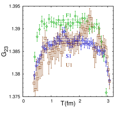
(a) $G_{23}$

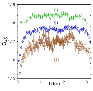
(b) $G_{45}$

Figure 1: $G_{23}$ and $G_{45}$ at renormalization scale $\mu=1/a$ as a function of $T$, the Euclidean time between the kaon source and operator insertion. (Green) diamond, (blue) pentagon, and (brown) square points are from the F1, S1, U1 ensembles, respectively, which all have similar sea-quark masses ($am_{\ell}/am_{s}=1/5$). The valence quarks satisfy $(m_{x},m_{y})=(m_{s}/10,m_{s})$.

On each ensemble, we first do the valence chiral extrapolation. This “X-fit” is done with respect to $X\equiv X_{p}/\Lambda^{2}_{\chi}$, with $\Lambda_{\chi}=1\mathop{\rm GeV}\nolimits$ and $X_{P}=m^{2}_{\pi}(x\bar{x})$ the valence $x\bar{x}$ meson mass-squared. For the G-parameters, the fitting function is

$$G_{i}(\text{X-fit})=c_{1}+c_{2}X+c_{3}X^{2}+c_{4}X^{2}\text{ln}^{2}X+c_{5}X^{2}\text{ln}X+c_{6}X^{3}\,,$$ (5)

which includes generic NNLO chiral logarithmic terms. We do correlated fits with Bayesian priors $c_{i}=0\pm 1$ for $c_{4-6}$. In the case of $B_{K}$, the fitting functional includes NLO chiral logs, and we follow the same fitting procedure as in Refs. [8, 9, 10].

We next do the “Y-fit”: an extrapolation in $Y\equiv Y_{P}/\Lambda^{2}_{\chi}$, with $Y_{P}=m^{2}_{\pi}(y\bar{y})$, to the “physical” $\eta_{s}(s\bar{s})$ mass. The central value is obtained by a linear fit. Example X- and Y-fits are shown in Fig.2.

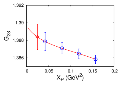
(a) X-fit

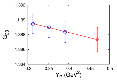
(b) Y-fit

Figure 2: Extrapolations of $G_{23}$ on the U1 ensemble, for operators renormalized at the scale $\mu=1/a$. The red points are extrapolated values.

The final step is to use all our ensembles to extrapolate to the physical values of the sea-quark masses and to the continuum limit. To do so, we must first evolve the matrix elements (or ratios) from $\mu=1/a$ to a common energy scale, $\mu=2\mathop{\rm GeV}\nolimits$ or $3\mathop{\rm GeV}\nolimits$, using the two-loop anomalous dimension matrix from Ref. [5]. We have discovered that, in Refs. [1, 2], we used the wrong value of the two-loop contribution to the anomalous dimension for the pseudoscalar operator. This enters through the denominators of the B-parameters [see Eq. (2)]. This error turns out to have a $\sim 5\%$ effect on the final results for BSM B-parameters. We have corrected this problem here.

fit type	fitting functional form	Bayesian Constraints
$F^{1}_{B}$	$d_{1}+d_{2}\frac{L_{P}}{\Lambda^{2}_{\chi}}+d_{3}\frac{S_{P}}{\Lambda^{2}_{\chi}}+d_{4}(a\Lambda_{Q})^{2}$	$d_{2}\cdots d_{4}=0\pm 2$
$F^{4}_{B}$	$F^{1}_{B}+d_{5}(a\Lambda_{Q})^{2}\frac{L_{P}}{\Lambda^{2}_{\chi}}+d_{6}(a\Lambda_{Q})^{2}\frac{S_{P}}{\Lambda^{2}_{\chi}}$
	$+d_{7}(a\Lambda_{Q})^{2}\alpha_{s}+d_{8}\alpha_{s}^{2}+d_{9}(a\Lambda_{Q})^{4}$	$d_{2}\cdots d_{9}=0\pm 2$
$F^{6}_{B}$	$F^{4}_{B}+d_{10}\alpha_{s}^{3}+d_{11}(a\Lambda_{Q})^{2}\alpha_{s}^{2}+d_{12}(a\Lambda_{Q})^{4}\alpha_{s}+d_{13}(a\Lambda_{Q})^{6}$
	$+d_{14}(a\Lambda_{Q})^{4}\frac{L_{P}}{\Lambda^{2}_{\chi}}+d_{15}(a\Lambda_{Q})^{2}\alpha_{s}\frac{L_{P}}{\Lambda^{2}_{\chi}}+d_{16}\alpha_{s}^{2}\frac{L_{P}}{\Lambda^{2}_{\chi}}$
	$+d_{17}(a\Lambda_{Q})^{4}\frac{S_{P}}{\Lambda^{2}_{\chi}}+d_{18}(a\Lambda_{Q})^{2}\alpha_{s}\frac{S_{P}}{\Lambda^{2}_{\chi}}+d_{19}\alpha_{s}^{2}\frac{S_{P}}{\Lambda^{2}_{\chi}}$	$d_{2}\cdots d_{19}=0\pm 2$

Table 2: Fitting functional forms for continuum-chiral extrapolation.

For the continuum-chiral extrapolation we use the fitting forms listed in Table 2. These are based on the power-counting rules for SU(3) SChPT, i.e. $L_{P}/\Lambda^{2}_{\chi}\approx S_{P}/\Lambda^{2}_{\chi}\approx(a\Lambda_{Q})^{2}\approx\alpha_{s}$, with $L_{P}$, $S_{P}$ the squared masses of the sea-quark pion and $\bar{s}s$ meson, respectively. Fit-form $F^{1}_{B}$ contains terms up to NLO, with the $\alpha_{s}$ term absent since we use 1-loop perturbative matching. $F^{4}_{B}$ contains all NNLO terms except those quadratic in $L_{P}$ and $S_{P}$. $F^{6}_{B}$ contains all NNNLO terms which are up to linear in quark masses.

In our previous work we used the simplest fitting form, $F^{1}_{B}$, to determine the central values of the extrapolated result [1, 2]. This continues to work well for $B_{K}$, $G_{21}$ and $G_{24}$, giving fits with $\chi^{2}/\text{dof}=1.08\sim 1.25$, as illustrated in Fig. 3(a). However, for $G_{23}$ and $G_{45}$, we find the addition of new ensembles leads to $F^{1}_{B}$ giving poor fits, and so we use fit $F^{4}_{B}$ instead for our central values. This gives reasonable fits, with $\chi^{2}/\text{dof}=1.32\sim 1.38$, as illustrated in Fig. 4.

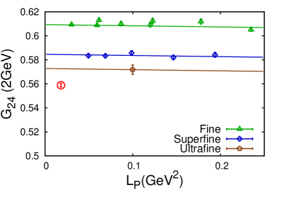
(a) $G_{24}$ fit by $F^{1}_{B}$, $\chi^{2}/\text{dof}=1.08$

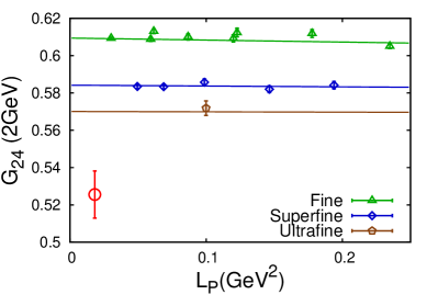
(b) $G_{24}$ fit by $F^{4}_{B}$, $\chi^{2}/\text{dof}=0.91$

Figure 3: Continuum-chiral extrapolation of $G_{24}$. Red circles are extrapolated results. Since values of $1/a$ and $S_{P}$ vary among ensembles with the same nominal lattice spacing, some scatter about the horizontal lines is expected, and this is accounted for in the fits [though not in the plot].

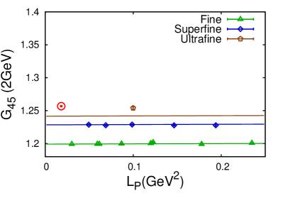
(a) $G_{45}$ fit by $F^{1}_{B}$ , $\chi^{2}/\text{dof}=4.06$

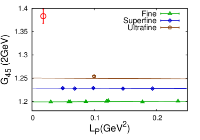
(b) $G_{45}$ fit by $F^{4}_{B}$ , $\chi^{2}/\text{dof}=1.38$

Figure 4: Continuum-chiral extrapolation of $G_{45}$. Notation as in Fig. 3.

We take the difference between $F_{1}^{B}$ and $F_{4}^{B}$ as the systematic uncertainty coming from the continuum-chiral extrapolation. It is a $\sim 1-8\%$ error. We compare it with our earlier estimate of the systematic error from one-loop perturbative matching ($\alpha_{s}^{2}(U1)\approx 4.4$%), and quote the larger as our estimate of the systematic error.

3 Discussion of results

The changes to our results since Lattice 2013 are summarized in Table 3. The first column shows the results presented last year in Refs. [1, 2]. The impact of adding new ensembles is shown in the second column, labeled “2014(ens)”, and is minor. The effect of correcting the two-loop pseudoscalar anomalous dimension is shown in the third column, labeled “2014(A.D.)”. This leads to $\sim 5\%$ reductions in the BSM B-parameters. Up to this stage the results are from $F_{1}^{B}$ fits. The final column shows the impact of switching to $F^{4}_{B}$ fits for $G_{23}$ and $G_{45}$ (necessitated by the poor quality of the $F_{1}^{B}$ fits). This changes $B_{3}$ and $B_{5}$ by $\sim 3\%$ and $9\%$, respectively.

B($\mu=3$GeV)	2013	2014(ens)	2014(A.D.)	2014(final)
$B_{K}$	0.519(7)(23)	0.518(3)	0.518(3)	0.518(3)(23)
$B_{2}$	0.549(3)(28)	0.547(1)	0.525(1)	0.525(1)(23)
$B_{3}$	0.390(2)(17)	0.390(1)	0.375(1)	0.358(4)(18)
$B_{3}^{\text{SUSY}}$	0.790(30)	0.783(2)	0.750(2)	0.774(6)(64)
$B_{4}$	1.033(6)(46)	1.024(1)	0.981(3)	0.981(3)(61)
$B_{5}$	0.855(6)(43)	0.853(3)	0.817(2)	0.748(9)(79)

Table 3: Changes to results during the last year. See text for discussion. Only statistical errors are shown in the second and third columns.

In Table 4 we show (in the first two columns) our preliminary results for two choices of renormalization scale $\mu$. The dominant error in the BSM B-parameters comes from the chiral-continuum extrapolation. For further details on the error budget, see Refs. [2, 10].

	SWME		RBC&UKQCD	ETM
	$\mu=2$GeV	$\mu=3$GeV	$\mu=3$ GeV	$\mu=3$ GeV
$B_{K}$	0.537(4)(24)	0.518(3)(23)	0.53(2)	0.51(2)
$B_{2}$	0.568(1)(25)	0.525(1)(23)	0.43(5)	0.47(2)
$B_{3}$	0.380(4)(19)	0.358(4)(18)	N.A.	N.A.
$B_{3}^{\text{SUSY}}$	0.849(6)(69)	0.774(6)(64)	0.75(9)	0.78(4)
$B_{4}$	0.984(3)(63)	0.981(3)(61)	0.69(7)	0.75(3)
$B_{5}$	0.712(9)(80)	0.748(9)(79)	0.47(6)	0.60(3)

Table 4: Comparison of results with those of RBC/UKQCD [3] and ETM [4] collaborations.

We also compare our results with those published by other collaborations. Results for $B_{K}$ and $B_{3}^{\rm SUSY}$ are consistent, those for $B_{2}$ differ at $\sim 2\sigma$, and those for $B_{4}$ and $B_{5}$ differ at $\sim 3\sigma$. These discrepancies, have, however, been reduced during the last year due to the changes summarized in Table 3.

The source of these discrepancies is not yet clear. We see two (related) places where we can improve our understanding of the systematic errors. First, we are using one-loop matching, whereas the other collaborations use non-perturbative renormalization (NPR). Our error estimate assumes a two-loop term of relative size $\alpha_{s}^{2}$, and this could be an underestimate. We are working towards using NPR to normalize our operators. Second, our continuum extrapolation is not fully satisfactory, as exemplified by the results in Fig. 4. The ultrafine ensemble lies further from the superfine and fine ensembles than is consistent with the simple $F^{1}_{B}$ fit-form, and this drives the fit in the right-hand panel to pick out relatively large coefficients for $\alpha_{s}^{2}$ terms. While this may be correct, it leads to a non-intuitive extrapolation. We hope to report further on these issues in the near future.

4 Acknowledgments

We are grateful to Claude Bernard and the MILC collaboration for private communications. C. Jung is supported by the US DOE under contract DE-AC02-98CH10886. The research of W. Lee is supported by the Creative Research Initiatives Program (No. 2014001852) of the NRF grant funded by the Korean government (MEST). W. Lee would like to acknowledge the support from KISTI supercomputing center through the strategic support program for the supercomputing application research (KSC-2013-G2-005). The work of S. Sharpe is supported in part by the US DOE grants no. DE-FG02-96ER40956 and DE-SC0011637.

References

- [1] T. Bae et al. PoS LATTICE2013 (2013) 473, [arXiv:1310.7372].
- [2] T. Bae et al. Phys.Rev. D88 (2013) 071503, [arXiv:1309.2040].
- [3] P. Boyle, N. Garron, and R. Hudspith Phys.Rev. D86 (2012) 054028, [arXiv:1206.5737].
- [4] V. Bertone et al. JHEP 1303 (2013) 089, [arXiv:1207.1287].
- [5] A. J. Buras, M. Misiak, and J. Urban Nucl.Phys. B586 (2000) 397–426, [hep-ph/0005183].
- [6] F. Gabbiani, E. Gabrielli, A. Masiero, and L. Silvestrini Nucl.Phys. B477 (1996) 321–352, [hep-ph/9604387].
- [7] J. Bailey, H.-J. Kim, W. Lee, and S. Sharpe Phys.Rev. D85 (2012) 074507, [arXiv:1202.1570].
- [8] T. Bae et al. Phys.Rev. D82 (2010) 114509, [arXiv:1008.5179].
- [9] T. Bae et al. Phys.Rev.Lett. 109 (2012) 041601, [arXiv:1111.5698].
- [10] T. Bae et al. Phys.Rev. D89 (2014) 074504, [arXiv:1402.0048].