Domain of attraction of saturated switched systems under dwell-time switching

Abstract

This paper considers discrete-time switched systems under dwell-time switching and in the presence of saturation nonlinearity. Based on Multiple Lyapunov Functions and using polytopic representation of nested saturation functions, a sufficient condition for asymptotic stability of such systems is derived. It is shown that this condition is equivalent to linear matrix inequalities (LMIs) and as a result, the estimation of domain of attraction is formulated into a convex optimization problem with LMI constraints. Through numerical examples, it is shown that the proposed approach is less conservative than the others in terms of both minimal dwell-time needed for stability and the size of the obtained domain of attraction.

This paper considers the computation of domain of attraction (DOA) of discrete-time switched systems with saturation nonlinearity in the form of

$$\left\{\begin{array}[]{l}x(t+1)=A_{\sigma(t)}\,x(t)+B_{\sigma(t)}sat(u(t))\\ \;\;\,\quad u(t)=K_{\sigma(t)}\,x(t)\end{array}\right.$$ (3)

where, $x\in\mathbb{R}^{n}$, $u\in\mathbb{R}^{m}$ are the state and control variables respectively. $\sigma(t):\mathbb{Z}^{+}\rightarrow\mathcal{I}_{N}:=\{1,\cdots,N\}$ is also a time-dependent switching signal that indicates the current active mode of the system among $N$ possible modes in $\mathcal{I}_{N}$. Symbol $sat(\cdot)$ is the standard vector-valued saturation function, i.e., $sat(u)=[sat(u_{1}),\cdots,sat(u_{m})]^{T}$, with $sat(u_{j})=sgn(u_{j})\min\{1,|u_{j}|\}$. Without loss of generality, the saturation limit is normalized to one, by appropriately scaling the $B_{\sigma}$ and $K_{\sigma}$ matrices.

The study of switched systems has been quite active in the past decade due to their potential in modeling of many practical real-life systems (see e.g. car transmission systems [1], multiple-controller systems [2], genetic regulatory networks [3], etc). Most of the literature of the switched systems is concerned with conditions that ensure stability of the system (3) in the absence of saturation and when $\sigma(\cdot)$ is an arbitrary switching function [4, 5, 6]. Others consider stability of switched systems when $\sigma(\cdot)$ satisfies some dwell-time restrictions [7, 8, 9, 10, 11, 12, 13].

Since most of the physical actuators/sensors are subject to hardware limitations, presence of control saturation is always inherent to control systems, which may cause stability loss and performance degradation. Moreover, computation and characterization of DOA of such systems is specially challenging as their DOA is known to be generally non-convex [14, 15]. Thus, estimation of DOA of switched systems in the presence of saturation nonlinearity has received the attention of many researchers (see, e.g., [16, 17, 18, 19]).

While several approaches have been proposed to handle saturation nonlinearity, two of them appear promising. The first approach is to describe the saturation nonlinearity as a local sector bound nonlinearity with different multipliers (see, e.g. [20, 21]). Then, the S-procedure is used to derive sufficient conditions for stability of the resulted nonlinear system. The second approach, is based on the polytopic representation of saturation nonlinearity [22, 23, 24], in which the saturation function is represented as a linear differential/difference inclusion (LDI). With this representation, conventional tools designed for linear systems can be used for saturated systems. It has been realized that the second approach generally leads to less conservative results [25]. Although the above mentioned approaches have been applied for switched systems under arbitrary switching (see e.g. [16, 17, 18, 26]), the extension of these methods for switched systems under dwell-time switching is not trivial due the complex structure of switching sequences that satisfy the dwell-time restriction. To the best of our knowledge there are very few results on such systems [27, 28].

This paper presents an LDI-based approach for computation of DOA of system (3) when $\sigma(\cdot)$ is a switching function that satisfies the dwell-time restriction. We formulate the problem into an optimization with linear matrix inequalities (LMI) constraints that asymptotically stabilizes system (3) and at the same time enlarges its DOA. We show that our result is less conservative than the others in terms of both minimal dwell-time needed for stability and the size of the obtained DOA.

In the limiting case, where the dwell-time is one sample period, $\sigma(\cdot)$ becomes an arbitrary switching function, and our method retrieves the results of arbitrary switched systems appeared in the literature (see, e.g., [16, 17]). Hence, this work can also be seen as a generalization of those obtained for arbitrary switched systems.

The rest of this paper is organized as follows. This section ends with a description of the notations used. Section I reviews some standard terminology and preliminary results for switched systems. Section II presents the main results including the LMI formulation of the problem. Sections III and IV contain, respectively, numerical examples and conclusions.

The following notations are used. $\mathbb{Z}^{+}$ is the set of non-negative integers. Given an integer $m\geq 1$, define $\mathcal{V}_{m}:=\{S:S\subseteq\{1,...,m\}\}$ as the set of all subsets of $\{1,...,m\}$. Clearly, $\{\emptyset\}\in\mathcal{V}_{m}$ and there are $2^{m}$ elements in the set $\mathcal{V}_{m}$. Also let $S^{c}=\{j\in\{1,...,m\}:j\notin S\}$ to be the complement of $S$ in $\{1,...,m\}$. Given $a>0$, the floor function $\lfloor a\rfloor$ is the largest integer that is less than $a$. The $p$-norm of a vector or a matrix is $\|\cdot\|_{p},p=1,2,\infty$ with $\|\cdot\|$ refers to the 2-norm and $\mathcal{B}_{r}:=\{x\in\mathbb{R}^{n}:\|x\|\leq r\}$ is a norm ball with radius $r$. Given a matrix $Y\in\mathbb{R}^{m\times n}$, $Y^{i\bullet}$ is the $i$-th row and $Y^{\bullet j}$ is the $j$-th column of $Y$ and $\mathcal{L}(Y):=\{x:\|Yx\|_{\infty}\leq 1\}=\{x:|Y^{i\bullet}x|\leq 1,\forall i=1,\cdots,m\}$. The transpose of a vector/matrix $X$ is denoted by $X^{T}$ and $I_{m}$ is the $m\times m$ identity matrix. Positive definite (semi-definite) matrix, $P\in\mathbb{R}^{n\times n}$, is indicated by $P\succ 0(\succeq 0)$, $\mathcal{E}(P):=\{x:x^{T}Px\leq 1\}$ and $\lambda_{\max}(P)$, $\lambda_{\min}(P)$ denote respectively the maximum and minimum eigenvalues of $P$. Other notations are introduced when they are needed.

I Preliminaries

This section begins with the standard definitions of systems under dwell-time switching and assumptions on the system, followed by preliminary stability results.

Definition 1

Let a switching sequence of (3) be denoted by $\mathcal{S}(t)=\left\{\sigma(t-1),\cdots,\sigma(1),\sigma(0)\right\}$ with switching instants at $t_{0},t_{1},\cdots,t_{k},\cdots$ with $t_{0}=0$ and $t_{k}<t_{{k+1}}$. System (3) has a dwell-time of $\tau$ if $t_{{k+1}}-t_{k}\geq\tau$ for all $k\in\mathbb{Z}^{+}$. In addition, any switching sequence that satisfies this condition is said to be dwell-time admissible (DT-admissible) with dwell-time $\tau$ and is denoted by $\mathcal{S}_{\tau}$.

System (3) is assumed to satisfy the following assumptions: (A1) $A_{i}+B_{i}K_{i}$ is discrete-time Hurwitz for all $i\in\mathcal{I}_{N}$; (A2) A value of $\tau\geq 1$ has been identified such that the unsaturated switched system (3) is asymptotically stable with dwell-time $\tau$.

Assumption (A1) defines the family of systems considered in this work and is a reasonable requirement. The presence of a minimal dwell-time that ensure asymptotic stability of system (3) is well-known [7, 8]. Hence, assumption (A2) is made out of convenience and poses no restriction. In addition, it is assumed that there is no control on the switching rule by the user, except that the switching rule satisfies the dwell-time consideration.

In order to provide stability conditions for system (3), additional notations are required. Consider the $i$-th mode of (3). Then the successor state of $x$, $F_{i}(x)$, under mode $i$ is

$$F_{i}(x)=A_{i}\,x+B_{i}\,sat(K_{i}x).$$ (4)

Repeating the above leads to

$$F_{i}^{2}(x) =F_{i}(F_{i}(x))=A_{i}F_{i}(x)+B_{i}\,sat(K_{i}F_{i}(x))$$

$$\;\;\vdots$$

$$F_{i}^{t}(x) =F_{i}(F_{i}^{t-1}(x))=F_{i}(F_{i}(\cdots F_{i}(x)))$$ (5)

where $F_{i}^{t}(x)$ is the state evolution of (3) after $t$-steps with $x(0)=x$ and $\mathcal{S}_{\tau}(t)=\{i,i,\cdots,i\}$. Using this definition, the following result which is based on the Multiple Lyapunov Functions (MLFs) provides a sufficient condition for asymptotic stability of the origin of system (3).

Theorem 1

Assume that, for some $\tau\geq 1$, there exists a collection of positive definite matrices $P_{i}\succ 0$ for each $i\in\mathcal{I}_{N}$ such that

$$\big{(}F_{i}(x)\big{)}^{T}P_{i}\,\big{(}F_{i}(x)\big{)}-x^{T}P_{i}\,x<0$$

$$\qquad\qquad\qquad\qquad\qquad\qquad\qquad\quad\forall x\neq 0,\forall i\in\mathcal{I}_{N}$$ (6)

$$\big{(}F_{i}^{\tau}(x)\big{)}^{T}P_{j}\,\big{(}F_{i}^{\tau}(x)\big{)}<x^{T}P_{i}\,x$$

$$\qquad\qquad\qquad\qquad\forall x\neq 0,\forall(i,j)\in\mathcal{I}_{N}\times\mathcal{I}_{N},i\neq j$$ (7)

Then, the equilibrium solution $x=0$ of saturated switched system (3) is globally asymptotically stable with dwell-time $\tau$.

Proof:

Consider any DT-admissible switching sequence with dwell-time $\tau$ in accordance with Definition 1. Without loss of generality, assume that $\sigma(t)=i$ for all $t\in[t_{k},t_{{k+1}})$ where $t_{{k+1}}=t_{{k}}+\Delta_{k}$ and $\Delta_{k}\geq\tau$. At $t_{{k+1}}$, system switches to mode $j$ and hence $\sigma(t_{{k+1}})=j$. Consider an associated Lyapunov function $V_{i}(x)=x^{T}P_{i}\,x$ for each mode $i\in\mathcal{I}_{N}$ and define $V(x(t)):=x(t)^{T}P_{\sigma(t)}x(t)$. From (6), it follows that $V(x(t+1))-V(x(t))=V_{i}(x(t+1))-V_{i}(x(t))<0$ is negative definite for all $t\in[t_{k},t_{{k+1}})$ along an arbitrary trajectory of (3) and thus there exists a $\lambda\in(0,1)$ and $\alpha>0$ such that

$$\|x(t)\|_{2}^{2}\leq\alpha\,\lambda^{t-t_{k}}\,V(x(t_{k})),\quad\forall t\in[t_{k},t_{{k+1}})$$ (8)

On the other hand, from (7) it follows that

$$V\big{(}x(t_{{k+1}})\big{)} =\big{(}F_{i}^{\Delta_{k}}(x(t_{k}))\big{)}^{T}P_{j}\,\big{(}F_{i}^{\Delta_{k}}(x(t_{k}))\big{)}$$

$$<\big{(}F_{i}^{(\Delta_{k}-\tau)}(x{(t_{k})})\big{)}^{T}P_{i}\,\big{(}F_{i}^{(\Delta_{k}-\tau)}(x{(t_{k})})\big{)}$$

$$<x(t_{k})^{T}P_{i}\,x(t_{k})=V\big{(}x(t_{k})\big{)}$$ (9)

where the second inequality follows from (6) and the fact that $\Delta_{k}-\tau\geq 0$. Equation (9) implies that there exists a $\mu\in(0,1)$ such that $V(x(t_{{k+1}}))<\mu V(x(t_{k}))$ and thus

$$V(x(t_{{k+1}}))<\mu^{k}\,V(x(0)),\quad\forall k\in\mathbb{Z}^{+}$$ (10)

This together with (8) imply that the equilibrium solution $x=0$ of (3) is asymptotically stable. ∎

While conditions (6) and (7) guarantee asymptotic stability of (3), they are not tractable due to the existence of nested saturation functions in $F_{i}^{\tau}(x)$. In the following section, the LDI representation of saturation function is explored to transform conditions of Theorem 1 into linear matrix inequality (LMI) constraints that can be efficiently solved with convex optimization routines.

II Main Results

The LDI approach is generalized in this section and is used for estimation of DOA of system (3) under dwell-time switching. LDI approach uses auxiliary terms and exploits their convex hull to represent the saturation function as summarized in the following lemma:

Lemma 1

[24] For any $S\in\mathcal{V}_{m}$, define $D_{S}$ to be the $m\times m$ diagonal matrix with diagonal elements $D_{S}(j,j)$, whose value is 1 if $\>j\in S$ and 0 otherwise. Also define $D_{S^{c}}={I}_{m}-D_{S}$. Then, for all $u\in\mathbb{R}^{m}$ and $v\in\mathbb{R}^{m}$ such that $\left|v_{j}\right|\leq 1$ for all $j=1,\cdots,m$:

$$sat(u)\in co\left\{D_{S^{c}}u+D_{S}\,v:\forall S\in\mathcal{V}_{m}\right\}$$ (11)

To illustrate the main idea of the LDI approach, consider any $u\in\mathbb{R}^{2}$ as an example. According to Lemma 1, for any $v=[v_{1},v_{2}]^{T}\in\mathbb{R}^{2}$ such that $|v_{1}|\leq 1,|v_{2}|\leq 1$, it follows that

$$sat\left(\begin{bmatrix}u_{1}\\ u_{2}\\ \end{bmatrix}\right)\in co\left\{\begin{bmatrix}u_{1}\\ u_{2}\\ \end{bmatrix},\begin{bmatrix}u_{1}\\ v_{2}\\ \end{bmatrix},\begin{bmatrix}v_{1}\\ u_{2}\\ \end{bmatrix},\begin{bmatrix}v_{1}\\ v_{2}\\ \end{bmatrix}\right\}.$$

In other words, the above lemma states that $sat(u)$ can be expressed as a convex hull of vectors formed by choosing some rows (those belonging to $S$) from $v$ and the rest (those belonging to $S^{c}$) from $u$. Using (11) and assuming that $u=K_{i}x$ and $v$ is replaced by some linear function $H_{i}\,x$, it follows that

$$sat(K_{i}\,x)\in co\left\{D_{S^{c}}K_{i}\,x+D_{S}\,H_{i}\,x:\forall S\in\mathcal{V}_{m}\right\}$$ (12)

for all $x\in\mathcal{L}(H_{i}):=\{x:|H_{i}^{j\bullet}x|\leq 1\}=\{x:\|H_{i}x\|_{\infty}\leq 1\}$. Now, for a given $S\in\mathcal{V}_{m}$ define

$$E_{i,H_{i}}\big{(}x,S\big{)}:=\Big{(}A_{i}+\sum_{j\in S^{c}}B_{i}^{\bullet j}K_{i}^{j\bullet}\Big{)}x+\Big{(}\sum_{j\in S}B_{i}^{\bullet j}H_{i}^{j\bullet}\Big{)}x$$ (13)

and it follows from (4), (12) and (13) that for every $x\in\mathcal{L}(H_{i})$

$$F_{i}(x)\in co\{E_{i,H_{i}}(x,S):\forall S\in\mathcal{V}_{m}\}$$ (14)

While the LDI representation of $F_{i}(x)$ appeared in (6) is easily obtained from Lemma 1, the characterization of $F_{i}^{\tau}(x)$ appeared in (7) is difficult as it consists of $\tau$ nested saturation functions. The rest of this section describes the characterization of $F_{i}^{t}(x)$ by introducing $t$ auxiliary variables $H_{i,1},\cdots,H_{i,t}$. Each of these variables are introduced for LDI representation of one of the nested saturations.

Consider $F_{i}^{2}(x)$ and suppose that $H_{i,1}$ and $H_{i,2}$ are associated for LDI representation of $sat(K_{i}x)$ and $sat(K_{i}F_{i}(x))$, respectively. Define

$$E_{i,H_{i,2}}\big{(}F_{i}(x),S\big{)}:=$$

$$\Big{(}A_{i}+\sum_{j\in S^{c}}B_{i}^{\bullet j}K_{i}^{j\bullet}\Big{)}F_{i}(x)+\Big{(}\sum_{j\in S}B_{i}^{\bullet j}H_{i,2}^{j\bullet}\Big{)}x\quad$$ (15)

Then, from (13)-(II), it follows that

$$F_{i}(x)\in co\{E_{i,H_{i,1}}(x,S_{1}):\forall S_{1}\in\mathcal{V}_{m}\},\forall x\in\mathcal{L}(H_{i,1})$$ (16)

$$F_{i}^{2}(x)=F_{i}(F_{i}(x))\in co\{E_{i,H_{i,2}}(F_{i}(x),S_{2}):\forall S_{2}\in\mathcal{V}_{m}\},$$

$$\qquad\qquad\qquad\qquad\qquad\qquad\qquad\quad\;\;\forall x\in\mathcal{L}(H_{i,2})$$ (17)

Since $F_{i}^{2}(x)$ is represented by the convex-hull of $E_{i,H_{i,2}}(F_{i}(x),S_{2})$, and $F_{i}(x)$ is by itself a convex-hull of $E_{i,H_{i,1}}(x,S_{1})$, it is straightforward (see Lemma 2 in the Appendix) to expand $F_{i}^{2}(x)$ as

$$F_{i}^{2}(x)\in co\{E_{i,H_{i,2}}\big{(}E_{i,H_{i,1}}(x,S_{1}),S_{2}\big{)}:\forall S_{1},S_{2}\in\mathcal{V}_{m}\},$$

$$\qquad\forall x\in\mathcal{L}(H_{i,1})\cap\mathcal{L}(H_{i,2}).$$ (18)

An example that illustrates this is given next. Consider a single-input system where $m=1$ and hence $\mathcal{V}_{m}=\{\{\emptyset\},\{1\}\}$. From (II), it follows that $E_{i,H_{i,2}}\big{(}E_{i,H_{i,1}}(x,S_{1}),S_{2}\big{)}$ takes one of the following four expressions, depending on the values of $S_{1},S_{2}\in\mathcal{V}_{m}$:

$$S_{1}=\{\emptyset\},S_{2}=\{\emptyset\}:\;E_{i,H_{i,2}}\big{(}E_{i,H_{i,1}}(x,\{\emptyset\}),\{\emptyset\}\big{)}=$$

$$\hskip 162.1807pt(A_{i}+B_{i}K_{i})^{2}x$$ (19)

$$S_{1}=\{\emptyset\},S_{2}=\{1\}:\;E_{i,H_{i,2}}\big{(}E_{i,H_{i,1}}(x,\{\emptyset\}),\{1\}\big{)}=$$

$$\hskip 108.12047ptA_{i}(A_{i}+B_{i}K_{i})x+B_{i}\,H_{i,2}\,x$$ (20)

$$S_{1}=\{1\},S_{2}=\{\emptyset\}:\;E_{i,H_{i,2}}\big{(}E_{i,H_{i,1}}(x,\{1\}),\{\emptyset\}\big{)}=$$

$$\hskip 55.48286pt(A_{i}+B_{i}K_{i})A_{i}\,x+(A_{i}+B_{i}K_{i})B_{i}\,H_{i,1}\,x$$ (21)

$$S_{1}=\{1\},S_{2}=\{1\}:\;E_{i,H_{i,2}}\big{(}E_{i,H_{i,1}}(x,\{1\}),\{1\}\big{)}=$$

$$\hskip 96.73936ptA_{i}^{2}\,x+A_{i}B_{i}\,H_{i,1}\,x+B_{i}\,H_{i,2}\,x$$ (22)

Note that each one of the above expressions is an affine function of $H_{i,1}x$, $H_{i,2}x$. Therefore, $F_{i}^{2}(x)$ which is the convex-hull of them, is also an affine function of $H_{i,1}x$ and $H_{i,2}x$. This is a key property used for the conversion of condition (7) into an LMI (see Section II-A).

Similar to the above procedure, by associating auxiliary matrices $H_{i,1}$, $H_{i,2}$, $\cdots$, $H_{i,t}$ to each one of the nested saturation functions appeared in $F_{i}^{t}(x)$, it follows that

$$F_{i}^{t}(x)\in co\Big{\{}E_{i,H_{i,t}}(\cdots(E_{i,H_{i,1}}(x,S_{1}),\cdots),S_{t}):\quad\;$$

$$\forall S_{1},\cdots,S_{t}\in\mathcal{V}_{m}\Big{\}},\;\forall x\in\mathcal{L}(H_{i,1})\cap\cdots\cap\mathcal{L}(H_{i,t}).$$ (23)

To simplify the notations of $F_{i}^{t}(x)$, let

$$E_{i}\,(x,S_{1}):=E_{i,H_{i,1}}(x,S_{1})$$

$$E_{i}^{2}(x,S_{1},S_{2}):=E_{i,H_{i,2}}\big{(}E_{i,H_{i,1}}(x,S_{1}),S_{2}\big{)}$$

$$\qquad\vdots$$

$$E_{i}^{t}(x,S_{1},\cdots,S_{t}):=E_{i,H_{i,t}}(\cdots(E_{i,H_{i,1}}(x,S_{1}),\cdots),S_{t})$$ (24)

With these notations, the following theorem provides an estimate of DOA of (3).

Theorem 2

Suppose for some $\tau\geq 1$, there exist a collection of $P_{i}\succ 0$ and matrices $H_{i,1},H_{i,2},\cdots,H_{i,\tau}\in\mathbb{R}^{m\times n}$ for each $i\in\mathcal{I}_{N}$ such that

$$\big{[}E_{i}(x,S_{1})\big{]}^{T}P_{i}\big{[}E_{i}(x,S_{1})\big{]}-x^{T}P_{i}\,x<0\qquad\;\;$$

$$\hskip 99.58464pt\forall x\neq 0,\forall i\in\mathcal{I}_{N},\forall S_{1}\in\mathcal{V}_{m}$$ (25)

$$\big{[}E_{i}^{\tau}(x,S_{1},\cdots,S_{\tau})\big{]}^{T}P_{j}\big{[}E_{i}^{\tau}(x,S_{1},\cdots,S_{\tau})\big{]}-x^{T}P_{i}\,x<0$$

$$\hskip 48.36967pt\forall x\neq 0,\forall i\neq j\in\mathcal{I}_{N},\forall S_{1},\cdots,S_{\tau}\in\mathcal{V}_{m}$$ (26)

$$\mathcal{E}(P_{i})\subseteq\mathcal{L}(H_{i,t})\hskip 42.67912pt\forall i\in\mathcal{I}_{N},t=1,2,\cdots,\tau$$ (27)

Then, (i) the origin of the saturated system (3) with dwell-time $\tau$ is locally asymptotically stable; (ii) $\Psi:=\bigcap_{i\in\mathcal{I}_{N}}\mathcal{E}(P_{i})$ is inside the DOA of (3).

Proof:

It is sufficient to show that for every $x\in\Psi$, equations (25)-(27) imply (6) and (7). To see this, consider any arbitrary $x\in\Psi=\cap_{i\in\mathcal{I}_{N}}\mathcal{E}(P_{i})$. From (27) it follows that $x$ is inside the polyhedral region $\mathcal{L}(H_{i,1})\cap\cdots\cap\mathcal{L}(H_{i,\tau})$ for all $i\in\mathcal{I}_{N}$. This and (16), imply that for every $x\in\Psi$, $F_{i}(x)=\sum_{S_{1}\in\mathcal{V}_{m}}\delta_{S_{1}}E_{i}(x,S_{1})$, for some $\delta_{S_{1}}\geq 0$ for each $S_{1}\in\mathcal{V}_{m}$ such that $\sum_{S_{1}\in\mathcal{V}_{m}}\delta_{S_{1}}=1$. Since $E_{i}(x,S_{1})^{T}P_{i}E_{i}(x,S_{1})$ is a convex function, we have

$$F_{i}(x)^{T}P_{i}F_{i}(x) =\big{[}\sum_{S_{1}}\delta_{S_{1}}E_{i}(x,S_{1})\big{]}^{T}P_{i}\big{[}\sum_{S_{1}}{\delta_{S_{1}}}E_{i}(x,S_{1})\big{]}$$

$$\leq\sum_{S_{1}}\delta_{S_{1}}\big{[}E_{i}(x,S_{1})^{T}P_{i}\,E_{i}(x,S_{1})\big{]}$$

$$<\sum_{S_{1}}\delta_{S_{1}}(x^{T}P_{i}\,x)=x^{T}P_{i}\,x$$

where the last inequality follows from (25).

Similarly, from (II) and (27) it is inferred that $F_{i}^{\tau}(x)=\sum_{S_{1},\cdots,S_{\tau}}\delta_{S_{1},\cdots,S_{\tau}}E_{i}^{\tau}(x,S_{1},\cdots,S_{\tau})$, for some $\delta_{S_{1},\cdots,S_{\tau}}\geq 0$, $S_{1},\cdots,S_{\tau}\in\mathcal{V}_{m}$ such that $\sum_{S_{1},\cdots,S_{\tau}}\delta_{S_{1},\cdots,S_{\tau}}=1$. Then from convexity of $E_{i}^{\tau}(x,S_{1},\cdots,S_{\tau})^{T}P_{j}E_{i}^{\tau}(x,S_{1},\cdots,S_{\tau})$ and (26), we have ${[F_{i}^{\tau}(x)]}^{T}P_{j}[F_{i}^{\tau}(x)]\leq\sum\delta_{S_{1},\cdots,S_{\tau}}\big{[}E_{i}^{\tau}(x,S_{1},\cdots,S_{\tau})^{T}P_{j}\,E_{i}^{\tau}(x,S_{1},\cdots,S_{\tau})^{\tau}\big{]}<\sum\delta_{S_{1},\cdots,S_{\tau}}(x^{T}P_{i}\,x\big{)}=x^{T}P_{i}\,x$.

Note that for every $x(0)\in\Psi$, $x(t)$ may move outside the $\Psi$ but condition (26) enforce that $x(t_{1})$ (after the first switching) be inside $\mu\Psi$ for some $\mu\in(0,1)$. In addition, condition (25) ensures that $x(t)$ remains inside the union of ellipsoids $\cup_{i\in\mathcal{I}_{N}}\mathcal{E}(P_{i})$ for all $t$. This, (26) and (27) together, imply that $x(t)$ is inside polyhedral regions $\bigcap_{i\in\mathcal{I}_{N}}\big{(}\mathcal{L}(H_{i,1})\cap\cdots,\mathcal{L}(H_{i,\tau})\big{)}$ for all $t\in\mathbb{Z}^{+}$ and hence LDI representation of (II) is valid at all times. ∎

Remark 1

In the limiting case where $\tau=1$, $\sigma(\cdot)$ becomes an arbitrary switching function and the conditions of Theorem 2 retrieves the stability results appeared in the literature for saturated systems under arbitrary switching (see e.g. [16, 18]).

Remark 2

Let $\bar{A}_{i}=A_{i}+B_{i}K_{i}$. Then, the conditions of Theorem 2 in the absence of saturation become

$$\bar{A}_{i}^{T}P_{i}\,\bar{A}_{i}-P_{i}\prec 0,\;\forall i$$ (28)

$$\big{[}\bar{A}_{i}^{\tau}\big{]}^{T}P_{j}\big{[}\bar{A}_{i}^{\tau}\big{]}-P_{i}\prec 0,\forall i\neq j$$ (29)

which is the stability condition for (unsaturated) switched system appeared in [11]. Thus, there indeed exist $P_{i}\succ 0$ and $H_{i,1},\cdots,H_{i,2\tau-1}$ that satisfy (25)-(26) so long as LMI (28)-(29) for system in the absence of saturation has a solution. This also signifies assumption (A2).

II-A LMI Formulation and Enlarging the Domain of Attraction

The estimate of DOA of system (3) obtained from Theorem 2 is the intersection of ellipsoidal sets $\mathcal{E}(P_{i})$. To enlarge the DOA, one must chose auxiliary matrices $H_{i,1},\cdots,H_{i,\tau}$ and $P_{i}$’s such that the volume of $\cap_{i\in\mathcal{I}_{N}}\mathcal{E}(P_{i})$ is maximized. This can be done by solving the following constrained optimization problem:

$$\max_{P_{i}\succ 0,H_{i,1},\cdots,H_{i,\tau}}\text{volume }\mathcal{E}(P_{i})$$

$$s.t.\;(\ref{eqn:MLF-E1}),(\ref{eqn:MLF-E2})\text{ and }(\ref{eqn:LH}).$$

In the sequel, we describe how to transform the above optimization problem into Linear Matrix Inequalities (LMIs) that can be efficiently solved with LMI solvers (see e.g. [29]).

The key point for this conversion is that $E_{i}^{t}(x,S_{1},\cdots,S_{t})$ for given $S_{1},S_{2},\cdots,S_{t}\in\mathcal{V}_{m}$, is an affine function of variable $H_{i,1}x,\cdots,H_{i,t}x$. This means that $E_{i}^{t}(x,S_{1},\cdots,S_{t})$ can be rewritten as

$$E_{i}^{t}(x,S_{1},\cdots,S_{t})=\Theta_{i,0}(S_{1},\cdots,S_{t})x+$$

$$\hskip 14.22636pt\Theta_{i,1}(S_{1},\cdots,S_{t})H_{i,1}\,x+\cdots+\Theta_{i,t}(S_{1},\cdots,S_{t})H_{i,t}\,x$$ (30)

where $\Theta_{i,\cdot}(S_{1},\cdots,S_{t})$’s are only functions of $A_{i},B_{i},K_{i}$ (see e.g. (19)-(22) for the expressions of $\Theta_{i,0}(S_{1},S_{2})$, $\Theta_{i,1}(S_{1},S_{2})$, $\Theta_{i,2}(S_{1},S_{2})$ for different values of $S_{1}$ and $S_{2}$). Hereafter, the dependence of $\Theta_{i,t}$ on $(S_{1},\cdots,S_{t})$ is dropped for notational convenience unless needed.

Now, to transform (26) into an LMI constraint, pre- and post-multiply it by $P_{i}^{-1}$. It follows that

$$x^{T}\Big{[}P_{i}^{-1}(\Theta_{i,0}+\cdots+\Theta_{i,\tau}H_{i,\tau})^{T}P_{j}(\Theta_{i,0}+\cdots+\Theta_{i,\tau}H_{i,\tau})P_{i}^{-1}$$

$$\hskip 28.45274pt-P_{i}^{-1}\Big{]}x<0\qquad\forall x\neq 0,\forall i\neq j$$ (31)

Let $Q_{i}=P_{i}^{-1},Y_{i,1}=H_{i,1}P_{i}^{-1},\cdots,Y_{i,\tau}=H_{i,\tau}P_{i}^{-1}$. Then, (II-A) is equivalent to

$$\big{(}\Theta_{i,0}Q_{i}+\cdots+\Theta_{i,\tau}Y_{i,\tau}\big{)}^{T}Q_{j}^{-1}\big{(}\Theta_{i,0}Q_{i}+\cdots+\Theta_{i,\tau}Y_{i,\tau}\big{)}$$

$$\hskip 156.49014pt-Q_{i}\prec 0\qquad\forall i\neq j$$

Utilizing the Schur complement, this can be converted into

$$\left[\begin{array}[]{cc}Q_{i}&*\\ \Theta_{i,0}Q_{i}+\cdots+\Theta_{i,\tau}Y_{i,\tau}&Q_{j}\end{array}\right]\succ 0 \forall i\neq j$$ (34)

where $*$ denotes the transpose of the off-diagonal term and (34) is now an LMI in terms of the variables $Q_{i},Q_{j},Y_{i,1},Y_{i,2},\cdots,Y_{i,\tau}$. Using the same procedure, constraint (25) is equivalent to

$$\left[\begin{array}[]{cc}Q_{i}&*\\ \Theta_{i,0}Q_{i}+\Theta_{i,1}Y_{i,1}&Q_{i}\end{array}\right]\succ 0 \forall i$$ (37)

Constraint (27) is also equivalent to the following LMI constraints [24]:

$$\;\mathcal{E}(P_{i})\subseteq\bigcap_{i\in\mathcal{I}_{N},t\in\{1,\cdots,\tau\}}\mathcal{L}(H_{i,t})\;\Leftrightarrow$$

$$\left[\begin{array}[]{cc}1&Y_{i,t}^{j\bullet}\\ &Q\end{array}\right]\succeq 0,\qquad\forall j\in\{1,\cdots,m\},\forall i\in\mathcal{I}_{N},$$ (40)

$$\qquad\qquad\qquad\qquad\quad\;\;\forall t\in\{1,\cdots,2\tau-1\}$$ (41)

where $Y_{i,t}^{j\bullet}$ is the $j$-th row of $Y_{i,t}$.

Finally, by using $tr(P_{i}^{-1})$ as a measure of size of the ellipsoid $\mathcal{E}(P_{i})$, the following corollary provides an approach for enlarging the DOA of (3).

Corollary 1

Suppose that for some $\tau\geq 1$, there exist matrices $Q_{i}\succ 0$ and $Y_{i,1},\cdots,Y_{i,\tau}$ for $i=1,2,\cdots,N$ such that the following linear matrix inequalities (LMIs) hold:

$$\left\{\begin{array}[]{l}\max_{Q_{i}\succ 0,Y_{i,1},\cdots,Y_{i,\tau}}\;\sum_{i=1}^{N}tr(Q_{i})\\ \\ \left[\begin{array}[]{cc}Q_{i}&*\\ \Theta_{i,0}(S_{1})Q_{i}+\Theta_{i,1}(S_{1})Y_{i,1}&Q_{i}\end{array}\right]\succ 0\\ \hskip 170.71652pt\forall i,\forall S_{1}\in\mathcal{V}_{m}\\ \\ \left[\begin{array}[]{cc}Q_{i}&*\\ \Theta_{i,0}(S_{1},\cdots,S_{\tau})Q_{i}+\cdots+\Theta_{i,t}(S_{1},\cdots,S_{\tau})Y_{i,\tau}&Q_{j}\end{array}\right]\succ 0\\ \hskip 113.81102pt\forall i\neq j,\forall S_{1},\cdots,S_{\tau}\in\mathcal{V}_{m}\\ \\ \left[\begin{array}[]{cc}1&Y_{i,t}^{j\bullet}\\ &Q_{i}\end{array}\right]\succeq 0\hskip 5.69054pt\forall i,\forall t\in\{1,\cdots,\tau\},\forall j\in\{1,\cdots,m\}\\ \end{array}\right.$$ (42)

Then, the origin of switched system (3) is locally asymptotically stable with dwell-time $\tau$ and $\Psi=\bigcap_{i\in\mathcal{I}_{N}}\mathcal{E}(Q_{i}^{-1})$ is the estimate of DOA. The auxiliary matrices $H_{i,t}$ are obtained from $H_{i,t}=Y_{i,t}P_{i}$ with $P_{i}=Q_{i}^{-1}$.

Remark 3

In the optimization problem (42), $\sum_{i}tr(Q_{i})$ is optimized over all possible matrices $H_{i,t},\cdots,H_{i,\tau}$, including $H_{i,t}=K_{i}$ for all $i\in\mathcal{I}_{N}$ and for all $t=1,\cdots,\tau$. Hence, the resulting DOA is no smaller than the one tangential to the sides of the unsaturated region, i.e. $\mathcal{L}_{K}:=\cap_{i\in\mathcal{I}_{N}}\{x:\|K_{i}x\|_{\infty}\leq 1\}$.

Remark 4

Any feasible solution of optimization problem (42) with dwell-time $\tau$, is also a feasible solution for optimization problem (42) with any $\bar{\tau}\geq\tau$. This means that $\Psi(\tau)$ is a DOA of (3) with dwell-time $\bar{\tau}\geq\tau$ and $\Psi(\tau)\subseteq\Psi(\bar{\tau})$.

III Numerical Example

The example considered is a single-input saturated switched system, taken from [28], with $\mathcal{I}_{N}=\{1,2\}$, $A_{1}=\left[\begin{smallmatrix}-0.7\;&\;\;\,1.0\\ -0.5\;&-1.2\end{smallmatrix}\right]$, $A_{2}=\left[\begin{smallmatrix}0.26\;&-1.0\\ 1.7\;&-1.5\end{smallmatrix}\right]$, $B_{1}=[1,\>0]^{T}$, $B_{2}=[0,\>-1]^{T}$, $K_{1}=[1.1759,\,0.1089]$, $K_{2}=[1.5114,\,-0.7765]$.

As LMIs (28)-(29) admit a solution with $\tau=2$, the system is asymptotically stable with dwell-time $\tau=2$ and thus assumption (A2) is satisfied for any $\tau\geq 2$. It can also be shown that the system is unstable under arbitrary switching and hence the methods proposed for arbitrary switched systems are not applicable for this example. The intention here is to compute an estimate of DOA of the system from Corollary 1 for different values of dwell-time $\tau\geq 2$ and compare them with the results presented in [28].

The solution of the optimization problem (42) with $\tau=2$ are $P_{1}=\left[\begin{smallmatrix}1.0839&1.5333\\ *&3.1411\end{smallmatrix}\right]$, $P_{2}=\left[\begin{smallmatrix}\;\;\;1.3408&-0.7720\\ *&\;\;\;1.2585\end{smallmatrix}\right]$, $H_{1,1}=[0.8898,0.7467]$, $H_{1,2}=[0.5660,1.5560]$, $H_{2,1}=[1.1270,-0.8560]$, $H_{2,2}=-[0.3050,0.4333]$. Figure 1 shows the corresponding ellipsoidal sets $\mathcal{E}(P_{1})$ and $\mathcal{E}(P_{2})$ and the polyhedral regions $\mathcal{L}(H_{1,1}),\mathcal{L}(H_{1,2}),\mathcal{L}(H_{2,1}),\mathcal{L}(H_{2,2})$. Note that $\mathcal{E}(P_{1})\subseteq\mathcal{L}(H_{1,1})\cap\mathcal{L}(H_{1,2})$ and $\mathcal{E}(P_{2})\subseteq\mathcal{L}(H_{2,1})\cap\mathcal{L}(H_{2,2})$ as imposed by (II-A). The DOA together with a sample trajectory of the system starting from $x(0)$ on the boundary of $\Psi=\mathcal{E}(P_{1})\cap\mathcal{E}(P_{2})$ under a periodic switching sequence is shown in Fig. 2. Note that $x(t)$ may move out of $\Psi$ (see $x(1),x(3)\notin\Psi$ in Fig. 2) but $x(t)$ remains in $\mathcal{E}(P_{1})\cup\mathcal{E}(P_{2})$ at all times. The corresponding Lyapunov function $V(x(t))=x(t)^{T}P_{\sigma(t)}x(t)$ is also shown in this figure. Again, $V(t)$ is not monotonically decreasing with respect to $t$ but $V(x(t_{k}))$ (the points marked with “o”) defines a monotonically decreasing sequence and thus $V(t)\rightarrow 0$ as $t\rightarrow\infty$.

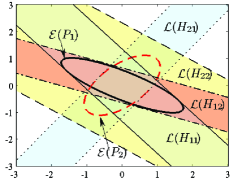
Figure 1: Illustration of $\Psi=\mathcal{E}(P_{1})\cap\mathcal{E}(P_{2})$ for $\tau=2$: $\mathcal{E}(P_{1})\subseteq\mathcal{L}(H_{1,1})\cap\mathcal{L}(H_{1,2})$ and $\mathcal{E}(P_{2})\subseteq\mathcal{L}(H_{2,1})\cap\mathcal{L}(H_{2,2})$;

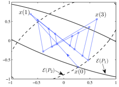
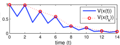
Figure 2: (top) State trajectory from $x(0)=(0.2763,-0.6918)$ on the boundary of $\Psi$ under a period switching with $\sigma(0)=2$, $t_{k+1}-t_{k}=2,\forall k$, (bottom) The Lyapunov function $V(x(t))$ and the monotonically decreasing sequence $V(x(t_{k}))$ at switching times.

III-A Comparison with other methods

As a comparison, the authors of [28] use an LDI-based method to obtain an estimate of DOA of (3). They show that if there exist $\lambda\in(0,1)$, $\mu\geq 1$, $P_{i}\succ 0$ and $H_{i}$ for each $i\in\mathcal{I}_{N}$ such that

$$[(E_{i,H_{i}}(x,S))]^{T}P_{i}\,[(E_{i,H_{i}}(x,S))]\leq\lambda\,x^{\top}P_{i}\,x$$

$$\hskip 128.0374pt\forall i\in\mathcal{I}_{N},\forall S\in\mathcal{V}_{m}$$ (43a)

$$P_{i}\preceq\mu\,P_{j}\hskip 85.35826pt\forall(i,j)\in\mathcal{I}_{N}\times\mathcal{I}_{N}$$ (43b)

$$\mathcal{E}(P_{i})\subseteq\mathcal{L}(H_{i})\hskip 105.27519pt\forall i\in\mathcal{I}_{N}$$ (43c)

Then, equilibrium solution $x=0$ of (3) is locally asymptotically stable with dwell-time $\tau\geq\lfloor-\frac{\ln\mu}{\ln\lambda}\rfloor$. For a fixed $\lambda$, conditions (43a) and (43c) can be easily converted into LMIs using the same procedure developed in Section II-A and optimized such that the size of $\mathcal{E}(P_{i})$’s are maximized. Then, an admissible choice of $\mu$ that satisfies (43b) is $\mu=\max_{i,j}\frac{\lambda_{\max}(P_{i})}{\lambda_{\min}(P_{j})}$. The estimate of DOA of this method is the largest norm-2 ball $\mathcal{B}_{r}=\{x:\|x\|\leq r\}\subseteq\cap_{i\in\mathcal{I}_{N}}\mathcal{E}(P_{i})$ such that if $x(0)\in\mathcal{B}_{r}$ then $x(t)\in\cap_{i\in\mathcal{I}_{N}}\mathcal{E}(P_{i})$ for all $t\in\mathbb{Z}^{+}$. An admissible choice of $r$ that guarantees this condition is $r=\min_{i\in\mathcal{I}_{N}}\frac{1}{\sqrt{\lambda_{max}(P_{i})}}$.

For the example considered in this section, the smallest dwell-time $\tau$ that results in a feasible solution for the optimization problem (43) is $\tau=5$. The resulting DOA, denoted by $\mathcal{B}_{r}$, is shown in Fig. 3 and compared with the DOA obtained from Corollary 1 with $\tau=5$.

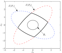
Figure 3: Comparison of DOA for $\tau=5$: $\mathcal{B}_{r}\subset\Psi=\mathcal{E}(P_{1})\cap\mathcal{E}(P_{2})$.

Computational results for different values of $\tau$ are also presented in Table I. These results include the size of DOA and the total number of LMIs involved in each method.

	Method of [28]		Corollary 1
$\tau$	$Area(\mathcal{B}_{r})$	# LMI	$Area(\Psi)$	# LMI
2	-	6	1.372	16
3	-	6	3.308	26
4	-	6	5.788	44
5	1.131	6	7.143	78
8	3.331	6	10.316	532

TABLE I: Computational results

From Table I, it can be seen that the proposed LDI approach is less conservative, in terms of both minimal dwell-time needed for stability and the size of DOA, than the LDI method of [28]. This is mainly because the variables $H_{i,1},\cdots,H_{i,\tau}$ gives us more freedom to characterize the polytopic representation of the solution of system (3) and hence enable us to find a larger estimate of DOA. Of course, this is possible at the expense of a more computational effort as the number of LMI constraints involved in (42) increases exponentially with $\tau$.

IV Conclusion

This paper proposes a sufficient condition for asymptotic stability of discrete-time switched systems under dwell-time switching and in the presence of saturation nonlinearity. This condition is shown to be equivalent to linear matrix inequalities (LMIs). As a result, the estimation of the domain of attraction is formulated into an optimization problem with LMI constraints. Through numerical examples, it is shown that our results are less conservative than the others, in terms of both minimal dwell-time needed for stability and the size of the obtained domain of attraction.

Lemma 2

Let $\alpha\in co\{\alpha_{i}:i=1,\cdots,n_{\alpha}\}$, $\beta\in co\{\beta_{j}:j=1,\cdots,n_{\beta}\}$ and $\gamma=\alpha+\beta$. Then, $\gamma\in co\{\alpha_{i}+\beta_{j}:i\in\{1,\cdots,n_{\alpha}\},j\in\{1,\cdots,n_{\beta}\}\}$.

References

[1]
K. H. Johansson, J. Lygeros, and S. Sastry, “Modelling hybrid systems,”
CONTROL SYSTEMS, ROBOTICS AND AUTOMATION in Encyclopedia of Life
Support Systems (EOLSS), vol. 43, no. 6, 2004.
[2]
A. S. Morse, “Supervisory control of families of linear set-point
controllers-part 1: Exact matching,” IEEE Trans. on Automatic
Control, vol. 41, no. 10, pp. 1413–1431, 1996.
[3]
H. D. Jong, J. Gouze, C. Hernandez, M. Page, T. Sari, and J. Geiselmann,
“Qualitative simulation of genetic regulatory networks using
piecewise-linear models. qualitative simulation of genetic regulatory
networks using piecewise-linear models,” Bulletin of Mathematical
Biology, vol. 66, no. 2, pp. 301–340, 2004.
[4]
J. Daafouz, P. Riedinger, and C. Iung, “Stability analysis and control
synthesis for switched systems: a switched lyapunov function approach,”
IEEE Trans. Automatic Control, vol. 47, no. 11, pp. 1883–1887, 2002.
[5]
F. Blanchini, S. Miani, and C. Savorgnan, “Stability results for linear
parameter varying and switching systems,” Automatica, vol. 43,
no. 10, pp. 1817–1823, 2007.
[6]
T. Hu and F. Blanchini, “Non-conservative matrix inequality conditions for
stability/stabilizability of linear differential inclusions,”
Automatica, vol. 46, no. 1, pp. 190–196, 2010.
[7]
G. Zhai, B. Hu, K. Yasuda, and A. N. Michel, “Qualitative analysis of
discrete-time switched systems,” in Proceedings of the American
Control Conference, Anchorage, Alaska, 2002, pp. 1880 – 1885.
[8]
M. Dehghan and C.-J. Ong, “Discrete-time switched linear system with
constraints: characterization and computation of invariant sets under
dwell-time consideration,” Automatica, vol. 48, no. 5, pp. 964–969,
2012.
[9]
F. Blanchini and P. Colaneri, “Vertex/plane characterization of the dwell-time
property for switching linear systems,” in Decision and Control (CDC),
2010 49th IEEE Conference on, 2010, pp. 3258 –3263.
[10]
M. Dehghan and C.-J. Ong, “Computations of mode-dependent dwell times for
discrete-time switching system,” Automatica, vol. 49, no. 6, pp.
1804–1808, 2013.
[11]
J. C. Geromel and P. Colaneri, “Stability and stabilization of discrete time
switched systems,” International Journal of Control, vol. 79, no. 7,
pp. 719–728, 2006.
[12]
G. Chesi, P. Colaneri, J. Geromel, R. Middleton, and R. Shorten, “A
nonconservative lmi condition for stability of switched systems with
guaranteed dwell time,” Automatic Control, IEEE Transactions on,
vol. 57, no. 5, pp. 1297–1302, may 2012.
[13]
M. Dehghan and C.-J. Ong, “Characterization and computation of disturbance
invariant sets for constrained switched linear systems with dwell time
restriction,” Automatica, vol. 48, no. 9, pp. 2175–2181, 2012.
[14]
T. Hu and Z. Lin, Control Systems with Actuator Saturation: Analysis and
Design. Birkhauser Boston, 2001.
[15]
Z. Sun, “Reachability analysis of constrained switched linear systems,”
Automatica, vol. 43, no. 1, pp. 164–167, 2007.
[16]
A. Benzaouia, L. Saydy, and O. Akhrif, “Stability and control synthesis of
switched systems subject to actuator saturation,” in Proceeding of the
American Control Conference, 2004, pp. 5818–5823.
[17]
A. Benzaouia, O. Akhrif, and L. Saydy, “Stabilization of switched systems
subject to actuator saturation by output feedback,” in IEEE Conference
on Decision and Control, 2006, pp. 777–782.
[18]
L. Lu and Z. Lin, “Design of switched linear systems in the presence of
actuator saturation,” IEEE Trans. Autom. Control, vol. 53, no. 6, pp.
1536–1542, 2008.
[19]
M. Dehghan, C.-J. Ong, and P. C. Y. Chen, “Enlarging domain of attraction of
switched linear systems in the presence of saturation nonlinearity,” in
ACC 2011, San Francisco, USA, 2011, pp. 1994–1999.
[20]
H. Khalil, Nonlinear systems, 3rd ed. Upper Saddle River, NJ: Prentice-Hall, 2002.
[21]
S. Tarbouriech, C. Prieur, and J. M. G. da Silva, “Stability analysis and
stabilization of systems presenting nested saturations,” IEEE
Transactions on Automatic Control, vol. 51, no. 8, pp. 1364–1371., 2006.
[22]
J. M. da Silva and S. Tarbouriech, “Local stabilization of discrete-time
linear systems with saturating controls: an lmi-based approach.” IEEE
Transactions on Automatic Control, vol. 46, no. 1, pp. 119–125, 2001.
[23]
T. Hu, Z. Lin, and B. Chen, “An analysis and design method for linear systems
subject to actuator saturation and disturbance,” Automatica, vol. 38,
no. 2, pp. 351 – 359, 2002.
[24]
——, “Analysis and design for discrete-time linear systems subject to
actuator saturation,” Systems & Control Letters, vol. 45, no. 1, pp.
97 – 112, 2002.
[25]
B. Zhou, W. X. Zheng, and G.-R. Duan, “An improved treatment of saturation
nonlinearity with its application to control of systems subject to nested
saturation,” Automatica, vol. 47, no. 2, pp. 306–315, 2011.
[26]
M. Jungers, E. B. Castelan, S. Tarbouriech, and J. Daafouz, “Finite
-induced gain and -contractivity of discrete-time switching
systems including modal nonlinearities and actuator saturations,”
Nonlinear Analysis: Hybrid Systems, vol. 5, pp. 289–300, 2011.
[27]
W. Ni and D. Cheng, “Control of switched linear systems with input
saturation,” Int Journal of Systems Science, vol. 41, no. 9, pp.
1057–1065, 2010.
[28]
Y. Chen, S. Fei, K. Zhang, and Z. Fu, “Control synthesis of discrete-time
switched linear systems with input saturation based on minimum dwell time
approach,” Circuits Syst Signal Process, vol. 31, 2012.
[29]
M. Grant and S. Boyd, “CVX: Matlab software for disciplined convex
programming,” 2011. [Online]. Available: http://cvxr.com